Adaptive Sparse Cyclic Coordinate Descent for Sparse Frequency Estimation

Abstract

The frequency estimation of multiple complex sinusoids in the presence of noise is important for many signal processing applications. As already discussed in the literature, this problem can be reformulated as a sparse representation problem. In this letter, such a formulation is derived and an algorithm based on sparse cyclic coordinate descent (SCCD) for estimating the frequency parameters is proposed. The algorithm adaptively reduces the size of the used frequency grid, which eases the computational burden. Simulation results revealed that the proposed algorithm achieves similar performance to the original formulation and the Root-multiple signal classification (MUSIC) algorithm in terms of the mean square error (MSE), with significantly less complexity.

1. Introduction

Parametric frequency estimation has been an active research area for many years. As a consequence, several methods have been proposed in the literature for addressing this problem. Among the most classic estimation strategies are the multiple signal classification (MUSIC) [1], its extension Root-MUSIC [2], and the estimation of signal parameters via rotational invariance techniques (ESPRIT) [3]. The principal drawback of these algorithms is their high computational complexity due to the required computation of the eigenvalue decomposition (EVD) of the measurement signal’s covariance matrix [4,5]. Furthermore, a degradation of the performance in scenarios with low signal to noise ratios (SNRs) can be also observed. Some approaches found in the literature, e.g., the work proposed in [6] for source localization, inspired the application of sparse representations in frequency estimation as an alternative method for overcoming the limitations of the classic techniques. As a consequence, some algorithms that exploit the sparse nature of the signals in the frequency domain have been introduced [7,8,9,10] in the literature. These methods rely on the sparse representation of the model. This means that the model assumes that the signal can be well-approximated as a linear combination of just a few underlying functions from a known basis or dictionary. Previous works based on these concepts using structured and dynamic dictionaries [11] have also been proposed. These algorithms have significant advantages, such as better performance compared with classic methods, less computational complexity, and more accurate results in scenarios with fewer available measurements.

The frequency estimation problem can be modeled as a linear combination of complex exponentials in the presence of noise via the following model:

$$\begin{array}{c}\hfill b\left[m\right]=\sum _{q=1}^p{x}_q{e}^{j2\pi f_{q}m}+w\left[m\right]\end{array}$$

(1)

where the coefficients $x_q$ represent the (complex) amplitudes, and $f_q$ are the frequencies of the signals. $w\left[m\right]$ represents the noise samples and p is the number of frequencies that are assumed to be known in this work.

Frequency estimation can be also formulated as a sparse representation problem using a sparse vector $\mathbf{x}$ of amplitudes, where the signal model in (1) can be rewritten using a frequency grid with a spacing of ${\Delta }_f$:

$$\begin{array}{c}\hfill \mathbf{b}=\mathbf{A}\mathbf{x}+\mathbf{w}.\end{array}$$

(2)

$\mathbf{b}$ represents the measurement vector of values $b\left[m\right]$, $\mathbf{w}$ the noise vector of values $w\left[m\right]$, and $\mathbf{A}$ is a $M\times N$ matrix with columns ${\mathbf{a}}_{*,i}={[e^{j2\pi i{\Delta }_{f}0},\dots ,e^{j2\pi i{\Delta }_{f}m},\dots ,e^{j2\pi i{\Delta }_{f}M-1}]}^T$. The measurement matrix $\mathbf{A}$ can be seen as a dictionary in which the columns represent complex exponentials with frequencies corresponding to points on a frequency grid. We assume normalized frequencies, i.e., a sampling frequency $f_s=1$ resulting in $f_s/2=0.5$, which naturally results in a number of columns $N=0.5/{\Delta }_f$ (assuming for simplicity that this fraction is an integer). For achieving high-precision estimation results, one should select a small ${\Delta }_f$, which leads to a large number of columns of $\mathbf{A}$, typically larger than the number of measurements M [12].

This representation encourages the use of sparse recovery algorithms. We present an approach that exploits this representation, leading to an algorithm that can be implemented efficiently in digital hardware, and is based on low complex coordinate rotation digital computer (CORDIC) operations. The proposed method is an extension of the sparse cyclic coordinate descent (SCCD) algorithm that significantly reduces the complexity further, allowing for efficient hardware implementations even for a large number of measurements. In contrast to, e.g., the Root-MUSIC algorithm that we will use for performance comparison, its complexity scales only quadratically in the number of measurements.

Sparse recovery algorithms can be classified into two principal categories: greedy algorithms (e.g., orthogonal matching pursuit (OMP) [13]; iterative hard thresholding (IHT) [14]) and convex optimization methods (least absolute shrinkage and selection operator (LASSO) [15], basis pursuit denoising (BPDN) [16], linearized Bregman iterations (LBI) [17], etc.). However, when choosing one of these algorithms for a particular application, there is a range of different properties that have to be considered, such as computational and storage requirements, ease of implementation, recovery performance, and flexibility [18]. An analysis of the performance guarantees of these algorithms usually involves quantities that measure the suitability of the measurement matrix $\mathbf{A}$ [19]. Some of these measures of quality are the restricted isometry property (RIP) and the mutual coherence (MC).

Greedy algorithms are easy to implement and can be extremely fast [18] in some scenarios. They ease the computational complexity by performing locally optimal greedy iterations, but the recovery guarantees are weaker than those of convex optimization methods. Successful estimation can only be guaranteed if one further assumes that all non-zero components of $\mathbf{x}$ are somewhat larger than the noise level. Greedy techniques rely on a least square (LS) solution for an estimated support, and this approach performs poorly unless the support is correctly identified. A single incorrectly identified element of the support can lead to the entire estimation being severely incorrect [20].

In the case of OMP, the performance guarantees rely on the RIP condition and the mutual coherence of the measurement matrix $\mathbf{A}$. In general, we do not normally know whether the RIP holds [18] and it is NP-hard to evaluate the restricted isometry constants (RICs) for a given matrix. They must then be bounded by efficiently computable properties of $\mathbf{A}$, such as the mutual coherence [20]. The exact recovery of every p-sparse vector via orthogonal matching pursuit is guaranteed when the measurement matrix has a coherence $\mu <1/(2p-1)$ [19]. The mutual coherence $\mu =\mu \left(\mathbf{A}\right)$ of a matrix $\mathbf{A}$ is defined as $\mu :={max}_{1\le i\ne j\le N}\left|\langle {\mathbf{a}}_i,{\mathbf{a}}_j\rangle \right|$ for a matrix $\mathbf{A}\in {\mathbb{C}}^{M\times N}$ with ${\ell }_2$-normalized columns for all $i\in \left[N\right]$ [19].

In applications such as frequency estimation where the measurement matrix is composed of complex exponentials that are highly correlated, conditions such as the one enunciated above are violated. For example, in a scenario with $M=50,{\Delta }_f=1/\left(20M\right)$ and $p=5$, the mutual coherence of the matrix $\mathbf{A}$ is equal to $0.9959$. Therefore this condition cannot be satisfied (i.e., $\mu =0.9959>1/(2p-1)=0.111$).

On the other hand, convex optimization methods have very good performance guarantees, which make them a reliable tool for sparse signal recovery but with the drawback that these methods typically have a higher computational cost for large-scale problems. Therefore, iterative approaches such as sparse cyclic coordinate descent (SCCD) [21] were introduced for solving these problems. SCCD is an optimization technique that sequentially minimizes a cost function in the direction of a single coordinate while leaving all other coordinates fixed. This is particularly useful in cases where the single parameter problem is easy to solve [22]. It is also especially suitable for problems where the gradient of the cost function does not have a closed-form solution. Moreover, efficient storage in a sparse vector format can be implemented since SCCD only updates one entry of the sparse vector at each iteration. SCCD also offers other advantages in terms of memory requirements compared to alternative algorithms such as linearized Bregman iterations. SCCD only uses a sparse vector of length N, and storing such a vector requires only a memory size depending on the number of non-zero values, whereas LBI requires an additional vector of length N which is dense and requires a most costly update [23,24]. Based on these characteristics, SCCD can be considered a more suitable candidate for the frequency estimation problem [12].

In this letter, a new version of SCCD based on an adaptive frequency grid is proposed. The proposed method inherits the characteristics of the original formulation and in addition employs several strategies for accelerating the convergence and reducing the number of required mathematical operations. The main idea of the proposed method is to effectively reduce the size of the grid (i.e., to reduce the number of columns of the matrix $\mathbf{A}$) for estimating the frequency parameters. This will allow one to reduce the computational complexity, and subsequently the number of required mathematical operations in comparison to the original formulation. Therefore, it enables a significantly better complexity/precision trade-off. As our approach mainly consists of complex rotations, it is easily implementable in fixed-point digital hardware with only moderate precision requirements. The proposed method also achieves similar performance to the Root-MUSIC algorithm, but with significantly less computational complexity.

2. Adaptive-Sparse Coordinate Descent Algorithm

The SCCD algorithm solves the following cost function:

$$\begin{array}{c}\hfill \underset{\mathbf{x}}{\arg \min }\frac{1}{2}{\parallel \mathbf{A}\mathbf{x}-\mathbf{b}\parallel }_2^2+\lambda {\parallel \mathbf{x}\parallel }_1,\end{array}$$

(3)

where the regularization parameter $\lambda$ is used to adjust the sparsity of the estimation result. Higher values of $\lambda$ lead to more sparse estimation results [12].

An interesting phenomenon occurs over the iterations in SCCD: most coordinates at each update that are zero never become nonzero [22]. This characteristic allows using different strategies to speed up the convergence of the algorithm. For example, one can use a vector of lambda in descending order instead of a fixed $\lambda$ [25]. Then, the estimation result of a higher $\lambda$ is used as the start value for the next estimation with a lower $\lambda$. Such a hot-starting strategy reduces the computational effort to obtain a whole solution path because the result of such a previous estimation provides a start vector for the next estimation that is typically closer to its solution than the all-zero vector. As a consequence, the computation of the final solution is considerably faster than computing the solution using a fixed arbitrary $\lambda$.

In [12], we proposed a version of SCCD for frequency estimation, where a decreasing strategy for updating the regularization parameter and a peak search are used for detecting the p frequencies exactly. This is repeated in Algorithm 1 for the reader’s convenience.

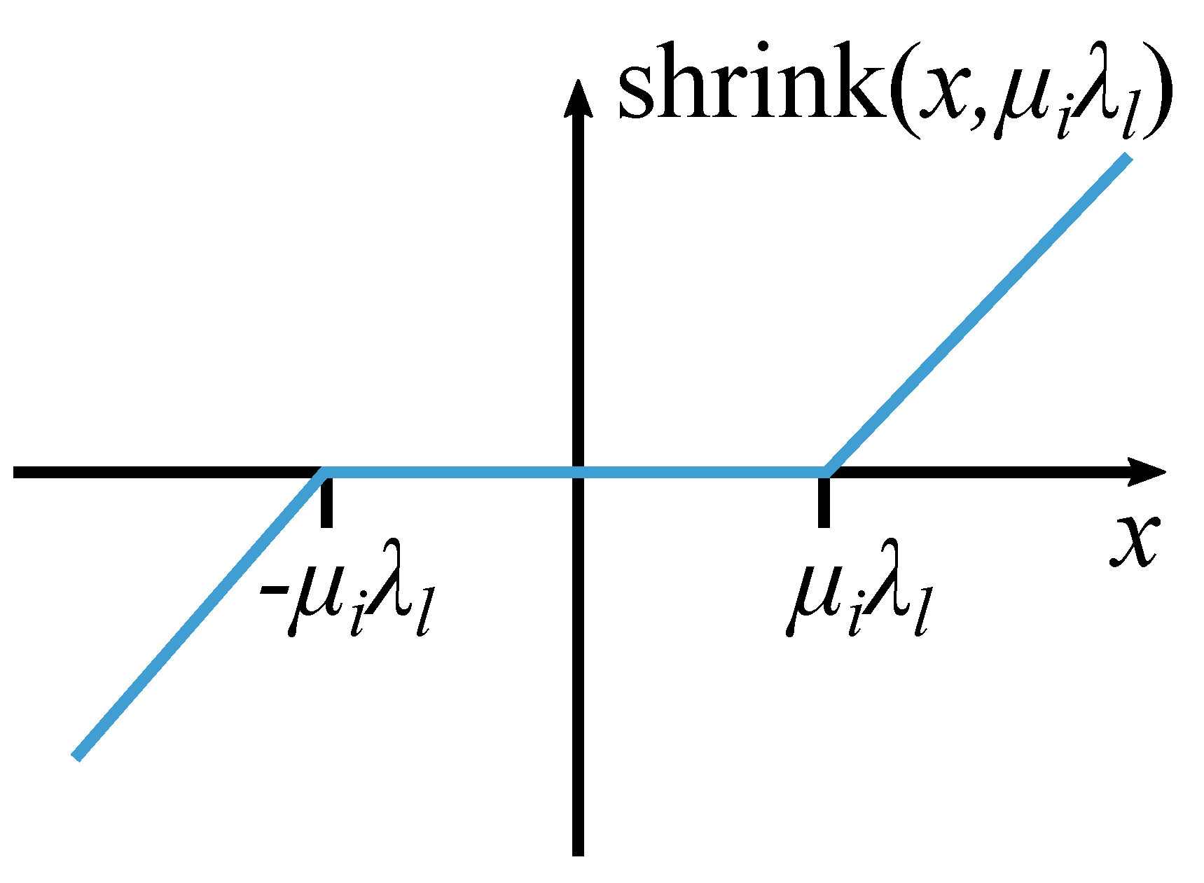
Algorithm 1 starts with a $\lambda$-value that would lead to the all-zero solution (i.e., ${\lambda }_1={\lambda }_{\max }$ where ${\lambda }_{\max }=\underset{i}{\max }\left|{\mathbf{a}}_{*,i}^H\mathbf{y}\right|$) [12] and reduces $\lambda$ until the number of estimated frequencies matches the desired number of frequencies p. For this, we use a vector of descending entries: $\lambda =[{\lambda }_1={\lambda }_{\max },{\lambda }_2,\dots ,{\lambda }_L]$. The iteration process basically consists of two principal steps. In the first step (line 8), the inner product between the corresponding column ${\mathbf{a}}_{*,i}$ and the residual $\mathbf{r}$ is computed and added to the currently estimated vector. Then, the resulting value is passed as the argument to the shrink function. The shrink function outputs zero if its input is smaller than a defined threshold (i.e., in our case smaller than ${\mu }_i{\lambda }_l$). If the input is larger than the threshold, the magnitude of the input is reduced by the threshold value. Figure 1 graphically depicts the shrink function. After applying the shrink function, the second step (line 9) of Algorithm 1 updates the residual.

In order to find an estimated vector with exactly p nonzero values that correspond to the true frequencies, a very fine grid of $\lambda$ values are required. This also implies a considerable increase in the number of iterations. In order to address this issue, a peak search on the estimated vector can be performed (line 11 of Algorithm 1). This allows detecting p frequencies, even when the number of nonzero elements of the estimated vector is larger than p. This strategy also allows using a relatively coarse vector of $\lambda$ values while still providing good estimation performance. The vector ${\mathbf{a}}_{*,i}$ in Algorithm 1 is composed of complex exponentials. Therefore, the inner product of such a vector with the vector $\mathbf{r}$ and the multiplication by a scalar (complex) number ${\mu }_i$ (line 8 of Algorithm 1) can be easily performed by the CORDIC algorithm without explicitly calculating and storing ${\mathbf{a}}_{*,i}$. Hence, the vector ${\mathbf{a}}_{*,i}$ will only exist virtually in the hardware implementation [12].

Based on Algorithm 1, we propose an extension of the work published in [12]. In the proposed version, we continue to exploit the fact that most coordinates that are zero remain unchanging over the iterations. This characteristic allows discarding the areas of the frequency grid that remain zero over the iterations. Then, the frequency grid can be redefined to the areas of interest where the values are nonzero. This dimensional reduction of the frequency grid considerably reduces the number of mathematical operations needed per iteration and speeds up the convergence of the algorithm. The proposed algorithm is called Adaptive-SCCD and consists of two main steps:

• In the first step, Algorithm 1 is run using a coarse grid. This means that the defined frequency spacing of the grid ${\Delta }_{f\mathrm{coarse}}$ uses a coarse grid spacing, which leads to a moderate number of columns of $\mathbf{A}$. After running the algorithm, the non-zero positions are detected. These positions are located in the non-zero intervals around the peaks of the estimated vector $\widehat{\mathbf{x}}$. This is the reason why we performed a peak search and detected the beginnings and ends of these intervals.
• In the second step, we again run Algorithm 1, but in this case, the frequency grid is constructed only considering the intervals detected in the first step and using a frequency spacing ${\Delta }_{f\mathrm{fine}}$. This considerably reduces the number of grid points (i.e., number of columns of the matrix $\mathbf{A}$) that need to be considered, resulting in a reduction of the required number of mathematical operations.

  Algorithm 1 Sparse cyclic coordinate descent (SCCD) for frequency estimation [12]
  Input:$\mathbf{b}$, $\lambda =[{\lambda }_1,\dots ,{\lambda }_L]$, ${\Delta }_f$, N, $\theta$, p
  Output:$\widehat{\mathbf{x}}$, set of detected frequencies
  1: ${\widehat{\mathbf{x}}}^{\left(0\right)}\leftarrow \mathbf{0}$
  2: $\mathbf{r}\leftarrow \mathbf{b}$
  3: $l=1$	▹ Index for $\lambda$
  4: for $k=1\dots K$ do	▹K as pre-set maximum of iterations
  5:    $i\leftarrow \left(\right(k-1\left)\mathrm{mod}N\right)+1$	▹ cyclic processing
  6:    ${\mathbf{a}}_{*,i}={[e^{j2\pi i{\Delta }_{f}0},\dots ,e^{j2\pi i{\Delta }_{f}m},\dots ,e^{j2\pi i{\Delta }_{f}M-1}]}^T$
  7:    ${\mu }_i\leftarrow 1/{∥{\mathbf{a}}_{*,i}∥}_2^2=1/M$
  8:    ${\widehat{x}}_i^{\left(k\right)}\leftarrow \mathrm{shrink}({\widehat{x}}_i^{(k-1)}+{\mu }_i{\mathbf{a}}_{*,i}^H\mathbf{r},{\mu }_i{\lambda }_l)$
  9:    $\mathbf{r}\leftarrow \mathbf{r}-{\mathbf{a}}_i({\widehat{x}}_i^{\left(k\right)}-{\widehat{x}}_i^{(k-1)})$
  10:    if $i=1$ and ${∥{\widehat{\mathbf{x}}}^k-{\widehat{\mathbf{x}}}^{k-N+1}∥}_1<\theta$ then
  11:        $P=\mathrm{AbsPeakPositions}\left({\widehat{\mathbf{x}}}^k\right)$
  12:        if $\left|P\right|<p$ then
  13:           $l\leftarrow \min (L,l+1)$
  14:        else return frequencies corresponding to P
  15:        end if
  16:    end if
  17: end for

The two main steps of the proposed algorithm are illustrated in Figure 2. The main advantage of this approach is that the first estimation (coarse search) allows finding intervals centered around the peaks. These intervals can be interpreted as the potential regions of the grid where the true frequencies can be located. Then, the size of the frequency grid is effectively reduced in the second step (fine search) by only considering the intervals detected before. As a consequence, the number of points of interest that need to be evaluated in the second step is reduced and the number of required mathematical operations also decreases.

The pseudocode of Adaptive-SCCD is described in Algorithm 2, where FindNonZeroPositions and BuildGrid are auxiliary functions. Note that in Figure 2, the intervals centered around the peaks of the absolute value of the estimated vector $\widehat{\mathbf{x}}$ correspond to the non-zero positions. The function FindNonZeroPositions finds the start and end values of these peaks and stores them in the vectors $\mathbf{s}$ and $\mathbf{e}$. The function is described in Algorithm 3. The function BuildGrid is used to build a fine frequency grid in the intervals found by the coarse estimation. The fine grid uses the frequency spacing ${\Delta }_{f\mathrm{fine}}$. It is described in more detail in Algorithm 4. Finally, the function SCCD_fine is used for estimating the frequency parameters using the fine frequency grid. This function is similar to the original one described in Algorithm 1, only the inner product of line 8 is now performed by only considering the non-zero intervals detected in the first run of SCCD. Then, for implementing the function SCCD_fine, the lines 5 and 6 in Algorithm 1 are replaced by

$$\begin{array}{c}\hfill \begin{array}{cc}\hfill & 5:\mathbf{for}i=1\dots N\mathbf{do}\hfill \\ \hfill & 6:{\mathbf{a}}_{*,i}={[e^{j2\pi \mathrm{grid\_fine}\left(i\right)0},\dots ,e^{j2\pi \mathrm{grid\_fine}\left(i\right)m},\dots ,e^{j2\pi \mathrm{grid\_fine}\left(i\right)M-1}]}^T.\hfill \end{array}\end{array}$$

Algorithm 2 Adaptive-SCCD for frequency estimation

Input:$\mathbf{b}$, $\lambda =[{\lambda }_1,\dots ,{\lambda }_L]$, $\theta$, $p,{\Delta }_f,{\Delta }_{f\mathrm{coarse}}$

Output: set of detected frequencies $\widehat{\mathbf{f}}$

1: $N=0.5/{\Delta }_{f\mathrm{coarse}}$

2: $\left[\widehat{\mathbf{x}}\right]$ = SCCD ($\mathbf{b}$, $\lambda$, ${\Delta }_{f\mathrm{coarse}}$, $N,\theta ,p$)

3: $[\mathbf{s},\mathbf{e}]$ = FindNonZeroPositions$(\widehat{\mathbf{x}},{\Delta }_{f\mathrm{coarse}}$)

4: ${\Delta }_{f\mathrm{fine}}={\Delta }_f$

5: $\mathrm{grid\_fine}=$ BuildGrid$(\mathbf{s},\mathbf{e}$, ${\Delta }_{f\mathrm{fine}})$

6: $N=\mathrm{size}\left(\mathrm{grid\_fine}\right)$

7: $[{\widehat{\mathbf{x}}}_{\mathrm{fine}},\widehat{\mathbf{f}}]$ = $\mathrm{SCCD\_fine}(\mathbf{b}$, $\lambda$, $\mathrm{grid\_fine}$, $N,\theta ,p$)

Algorithm 3 FindNonZeroPositions

Input:$\widehat{\mathbf{x}},{\Delta }_{f\mathrm{coarse}}$

Output:$\mathbf{s},\mathbf{e}$

1: $f_{\mathrm{grid}}=0:{\Delta }_{f\mathrm{coarse}}:0.5$

2: $\left[\mathrm{pks},\mathrm{loc}\right]=\mathrm{AbsPeakPositions}\left(\widehat{\mathbf{x}}\right)$

3: $\tilde{\mathbf{x}}=\mathrm{abs}\left(\widehat{\mathbf{x}}\right)$

4: $\mathrm{dx}=\left[0\mathrm{diff}\left(\tilde{\mathbf{x}}\right)\right]$

5: $P=\mathrm{length}\left(\mathrm{pks}\right)$

6: $\mathrm{start}=\mathrm{zeros}(P,1)$

7: $\mathrm{end}=\mathrm{zeros}(P,1)$

8: for $k=1\dots P$ do

9:     $\mathrm{start}=\mathrm{find}((f_{\mathrm{grid}}<f_{\mathrm{grid}}\left(\mathrm{loc}\left(k\right)\right))\&(\mathrm{dx}<=0))$

10:    if isempty(start) then

11:         start = 1

12:    end if

13:    $\mathbf{s}\left(k\right)=\mathrm{start}$

14:    $\mathrm{end}=\mathrm{find}((f_{\mathrm{grid}}>f_{\mathrm{grid}}\left(\mathrm{loc}\left(k\right)\right))\&(\mathrm{dx}>=0))$

15:    if isempty(end) then

16:         end = 1

17:    end if

18:    $\mathbf{e}\left(k\right)=\mathrm{end}$

19: end for

Algorithm 4 Buildgrid

Input:$\mathbf{s},\mathbf{e},{\Delta }_{f\mathrm{fine}}$

Output:$\mathrm{grid\_fine}$

1: $\mathrm{grid\_fine}=\left[\right]$

2: $f_{\mathrm{grid}}=0:{\Delta }_{f\mathrm{fine}}:0.5$

3: $\mathrm{grid\_endpoint}=\mathrm{sort}\left(f_{\mathrm{grid}}\left(\mathbf{e}\right)\right)$

4: $\mathrm{grid\_startpoint}=\mathrm{sort}\left(f_{\mathrm{grid}}\left(\mathbf{s}\right)\right)$

5: for $j=1\dots \mathrm{length}\left(\mathbf{s}\right)$ do

6:    $\mathrm{grid\_fine}=[\mathrm{grid\_fine},\mathrm{grid\_startpoint}\left(j\right):{\Delta }_{f\mathrm{fine}}:\mathrm{grid\_endpoint}\left(j\right)]$

7: end for

3. Results

The performance of our method in the following estimation scenarios is evaluated in terms of the mean square error (MSE).

$$\mathrm{MSE}=\frac{1}{Rp}\sum _{r=1}^R\sum _{i=1}^p{|{\widehat{f}}_{i,r}-f_i|}^2$$

(4)

between the correct frequencies $f_i$, $i=1,2,\dots ,p$ and their estimates ${\widehat{f}}_{i,r}$ in $R=1000$ runs. The measurement noise samples were drawn from an i.i.d. complex Gaussian random process with zero mean and variance ${\sigma }^2$.

The measurements have been created by summing p real sinusoids with phase $\varphi$ uniformly distributed at random in the interval $(0,2\pi )$ and the amplitudes were chosen randomly to be $-1$ or 1 for all the simulations. The vector $\lambda$ is defined as $\lambda =[{\lambda }_{\max },ϵ{\lambda }_{\max },{ϵ}^2{\lambda }_{\max },\dots ,{ϵ}^{(L-1)}{\lambda }_{\max }]$ where $ϵ=0.99$ and $L=50$. In the case of SCCD, we considered a frequency grid with a spacing of ${\Delta }_f=1/\left(20M\right)$, and for Adaptive-SCCD we consider a coarse grid with ${\Delta }_{f\mathrm{coarse}}=1/\left(2M\right)$ for the first step and in the second step a spacing equal to the original version (i.e., ${\Delta }_{f\mathrm{fine}}={\Delta }_f=1/\left(20M\right)$). We also included the following algorithms for comparison: Root-MUSIC; ESPRIT, whose code is available in [26]; discrete-time Fourier transform (DTFT); and the two-step iterative shrinkage/thresholding (TwIST) algorithm [27], whose code is available in [28]. The simulation results for Root-MUSIC were obtained using the function rootmusic built in MATLAB and considering autocorrelation matrices of size $M/2\times M/2$ for Root-MUSIC and also for ESPRIT. In the case of the algorithm TwIST, the parameter $\tau$ was set to 5.

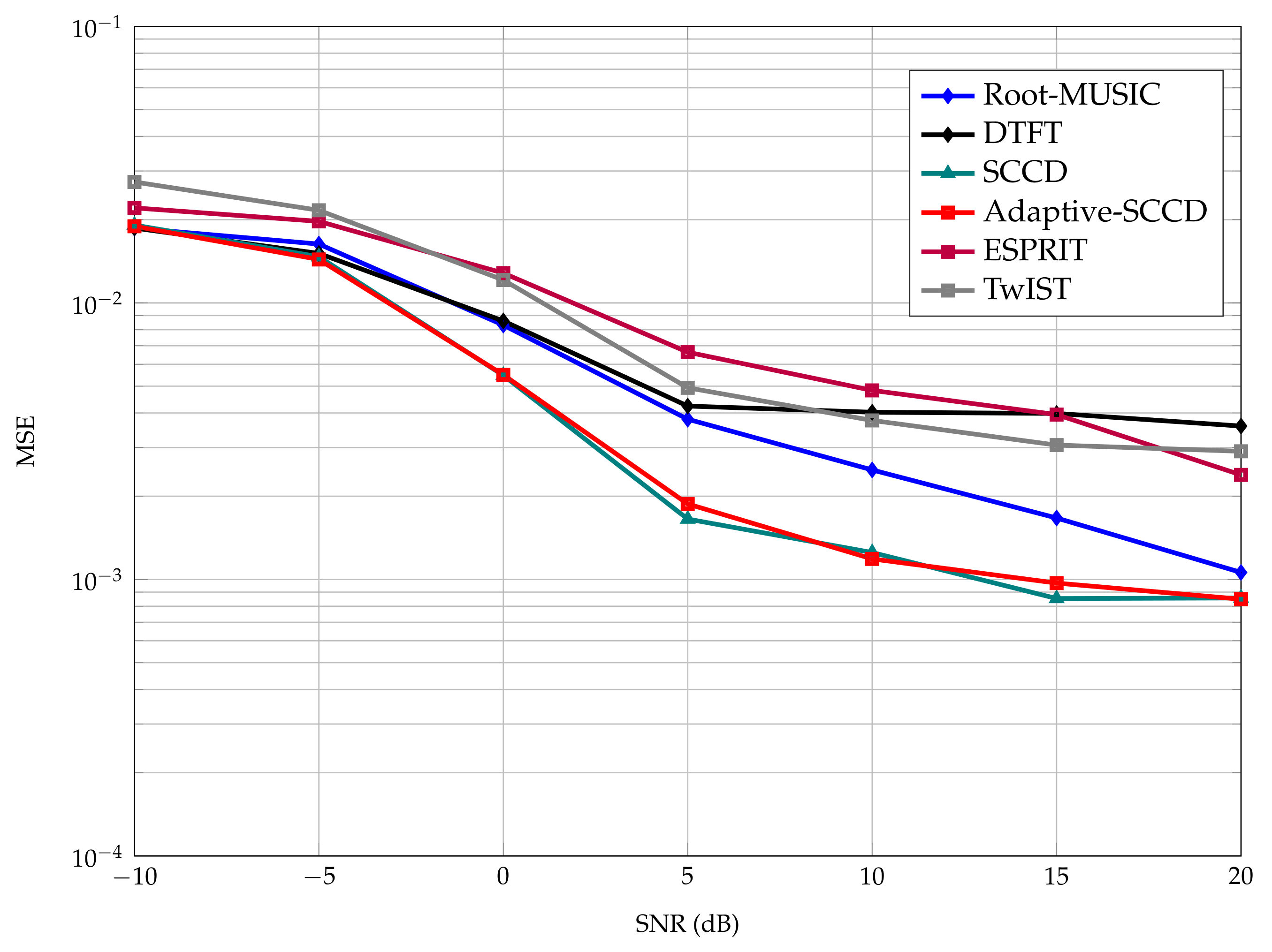
Figure 3 depicts a scenario with $M=50$ and five frequencies selected at random from the interval $(0,0.5)$. Please note that Adaptive-SCCD showed about the same performance as the original version of SCCD. This validates our affirmation that the adaptive reduction of the frequency grid size does not affect the final performance. Both versions of SCCD also outperformed the Root-MUSIC, ESPRIT, DTFT, and TwIST algorithms for this test case. In the case of the DTFT, it is known that in the presence of multiple frequencies, the DTFT suffers from spectral leakage due to interference among the sinusoidal components [29], which causes it to become biased [30]. Its inferior performance in this scenario was expected. In the case of the subspace techniques, Root-MUSIC showed the best performance compared to ESPRIT and is comparable in performance to Adaptive-SCCD. The performance gap between Root-MUSIC and ESPRIT is due to the fact that they work in different subspaces: Root-MUSIC works in the noise subspace with dimensions $M-p$, and ESPRIT works in the signal subspace with dimension p. Moreover, TwIST is an interesting approach based on the iterative shrinkage/thresholding (IST) algorithm that was originally proposed for image restoration, but we can notice that its performance for the simulated scenario of frequency estimation was inferior to Root-MUSIC and the proposed method.

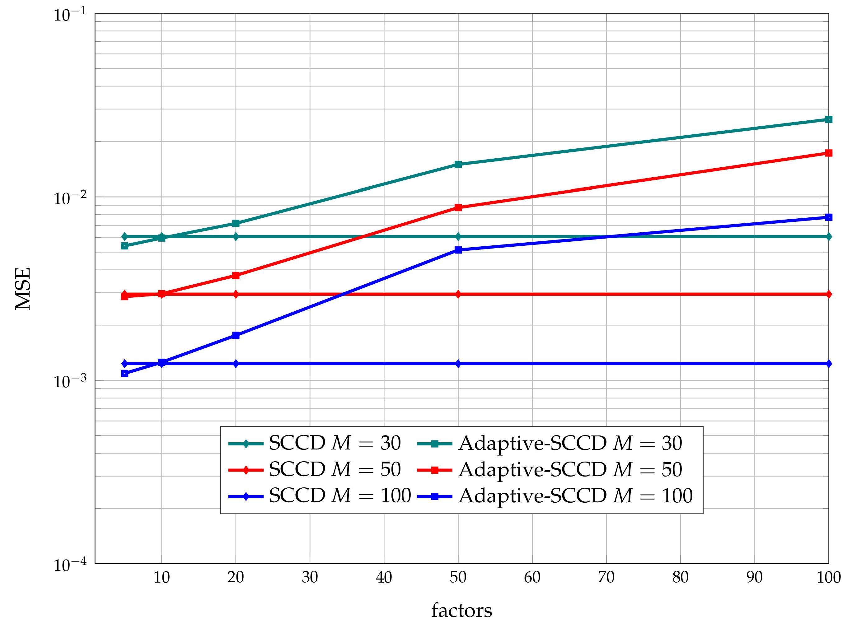
We also analyzed how the selection of ${\Delta }_{f\mathrm{coarse}}$ affects the final performance. We experimentally determined that a minimum spacing ${\Delta }_{f\mathrm{coarse}}=(1/2M)$ is necessary to guarantee the same final performance than SCCD. Figure 4 shows the performance of the original formulation versus the adaptive version for different values of ${\Delta }_{f\mathrm{coarse}}$. In the simulations, ${\Delta }_{f\mathrm{coarse}}=\mathrm{factor}·(1/\left(20M\right))$. This is the reason why the figure is represented as a function of the factors. In the case of SCCD, the spacing of the grid ${\Delta }_f=1/\left(20M\right)$ was always the same for all simulations.

Note that for values of ${\Delta }_{f\mathrm{coarse}}>(1/2M)$, i.e., factor values greater than 10, the performance of Adaptive-SCCD was worse than the performance of SCCD. This behavior was due to the fact that large values of ${\Delta }_{f\mathrm{coarse}}$ lead to a very coarse frequency grid. This produces scenarios with $M>N$ or even $N\le p$, where the coarse estimation fails to find all the intervals of interest (i.e., some parts of the grid where the true frequencies are located can not be detected in the coarse search). Therefore, some of these intervals of interest were excluded in the fine frequency grid. As a consequence, the Adaptive-SCCD algorithm was unable to estimate the true frequencies in the fine search.

As expected, we also observed in the simulation results that for larger values of M, the final performance improved, but we must consider that the increase of M also had an impact on the number of overall required computations. In [12], we outlined that the Algorithm 1 can be efficiently implemented in hardware using the CORDIC algorithm. In order to evaluate how the increase of the number of measurements impacts the complexity of such an implementation, we provide Figure 5.

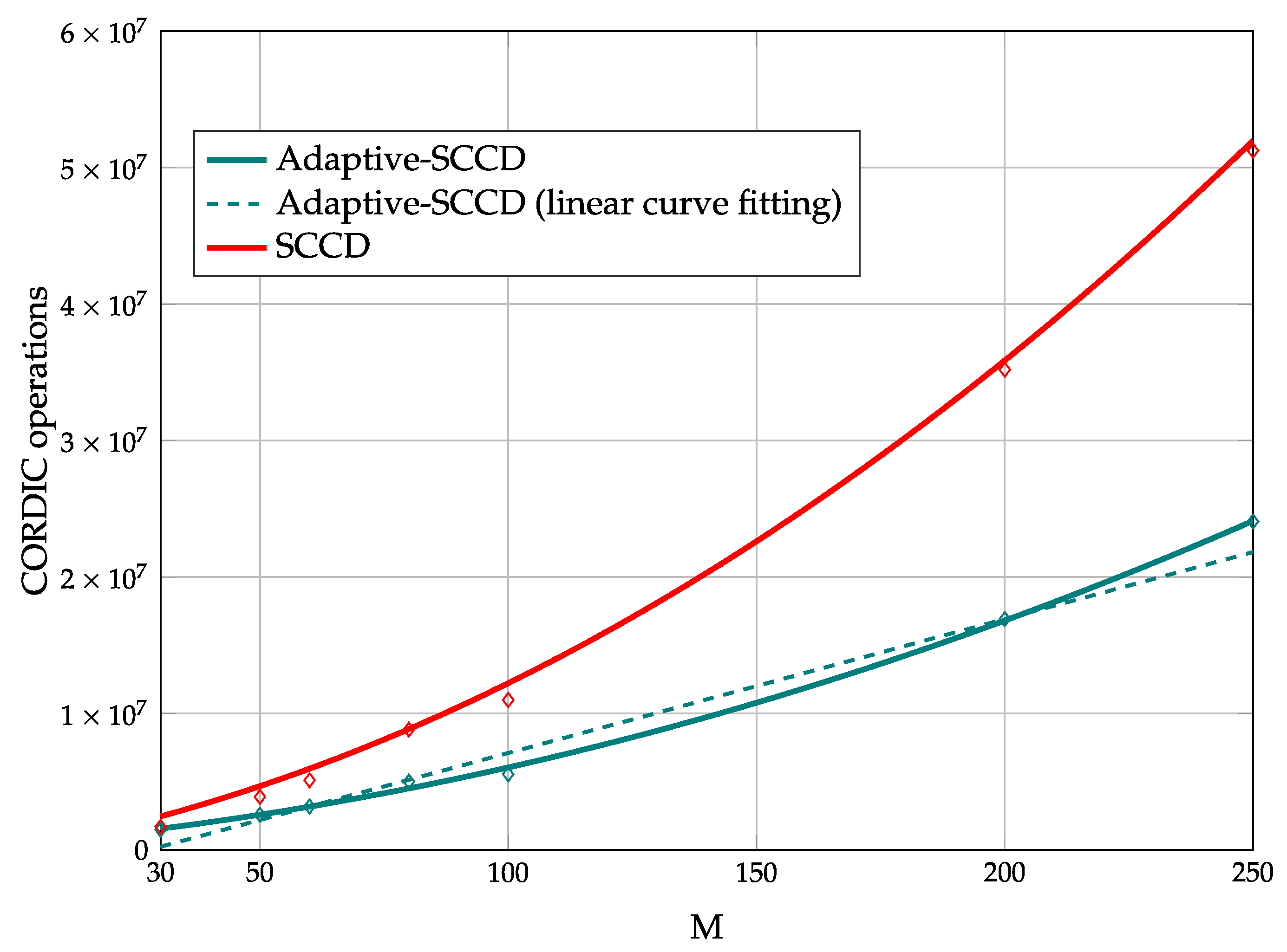
Figure 5 shows the average numbers of required CORDIC operations of SCCD and Adaptive-SCCD for different numbers of measurements. We considered the total number of iterations until the algorithms finished. A second-order polynomial in M has been used to fit the points with resulting $R^2$ (R-squared) values of 0.9988 and 0.9997 for Adaptive-SCCD and SCCD, respectively. In addition, a first-degree polynomial fitting for Adaptive-SCCD is also shown with an $R^2$ (R-squared) value of 0.9834. Note that the complexity of Adaptive-SCCD is significantly smaller than SCCD whenever the number of measurements increases. This result confirms that the proposed technique significantly reduces the computational complexity of the original formulation and provides a more efficient alternative for hardware implementations. Moreover, the subspace method MUSIC has a computational complexity of $\mathcal{O}(M^{2}N+M^2)$ [31]. As typically the number of grid points $N\gg M$, the complexity can be approximated to $\mathcal{O}\left(M^3\right)$. This implies that the computational cost of MUSIC scales cubically with respect to the number of measurements while the complexity of Adaptive-SCCD only scales quadratically in the number of measurements. Therefore, a significant complexity gap should be expected between an implementation of the MUSIC algorithm in digital hardware and the proposed method in scenarios where the number of measurements increases.

4. Materials and Methods

The implementations were written in MATLAB 2008a and simulations were run on an HP laptop running Windows 10 64-bit with an Intel(R) Core(TM) i7-7600 CPU and 16 GB of memory.

5. Conclusions

We proposed an adaptive algorithm based on SCCD for the frequency estimation problem that requires significantly less computational effort than its basic version. The proposed method relies on the sparse representation of the signal model, where the signal is represented as a multiplication of a measurement matrix A with a sparse vector. In order to estimate these frequencies, we proposed a method that effectively reduces the size of the frequency grid and considerably reduces the overall computational complexity without loss in performance. Moreover, the complexity of the method only scales quadratically with the number of measurements, while for other alternative methods, such as Root-MUSIC, it scales cubically. Basically, an implementation of Adaptive-SCCD in digital hardware will mostly consist of CORDIC operations and additions. This will result in a significant complexity gap between digital hardware implementations of Root-MUSIC and the proposed method. Due to the structure of the algorithm, designs can be efficiently implemented using sparse vector formats. Simulations have also shown that the proposed estimator achieves similar results in terms of the MSE to the original version, and outperforms other techniques such as Root-MUSIC.

The use-cases of a low-complexity and high-precision sparse frequency estimation method are manifold, including real-time applications in areas such as audio signal processing, radar or communications.

References

- Schmidt, R. Multiple emitter location and signal parameter estimation. IEEE Trans. Antennas Propag. 2011, 34, 276–280. [Google Scholar] [CrossRef] [Green Version]
- Rao, B.D.; Hari, K.V.S. Performance Analysis of Root-MUSIC. IEEE Trans. Acoust. Speech Signal Process. 1989, 37, 1939–1949. [Google Scholar] [CrossRef]
- Roy, R.; Kailath, T. ESPRIT-estimation of signal parameters via rotational invariance techniques. IEEE Trans. Acoust. Speech Signal Process. 1989, 37, 984–995. [Google Scholar] [CrossRef] [Green Version]
- Stoica, P.; Moses, R.L. Spectral Analysis of Signals; Prentice Hall, Inc.: Upper Saddle River, NJ, USA, 2005. [Google Scholar]
- Haardt, M.; Nossek, J.A. Unitary ESPRIT: How to obtain increased estimation accuracy with a reduced computational burden. IEEE Trans. Signal Process. 1995, 43, 1232–1242. [Google Scholar] [CrossRef]
- Malioutov, D.; Çetin, M. Sparse Signal Reconstruction Perspective for Source Localization with Sensor Arrays. IEEE Trans. Signal Process. 2005, 53, 3010–3022. [Google Scholar] [CrossRef] [Green Version]
- Angelosante, D.; Giannakis, G.B.; Sidiropoulos, N.D. Estimating Multiple Frequency-Hopping Signal Parameters via Sparse Linear Regression. IEEE Trans. Signal Process. 2010, 58, 5044–5056. [Google Scholar] [CrossRef] [Green Version]
- Liu, S.; Hu, Q.; Li, P.; Zhao, J.; Wang, C.; Zhu, Z. Speckle Suppression Based on Sparse Representation with Non-Local Priors. Remote Sens. 2018, 10, 439. [Google Scholar] [CrossRef]
- Liu, S.; Liu, M.; Li, P.; Zhao, J.; Zhu, Z.; Wang, X. SAR Image Denoising via Sparse Representation in Shearlet Domain Based on Continuous Cycle Spinning. IEEE Trans. Geosci. Remote Sens. 2017, 55, 2985–2992. [Google Scholar] [CrossRef]
- Liu, Y.; Chen, X.; Ward, R.K.; Wang, Z.J. Medical Image Fusion via Convolutional Sparsity Based Morphological Component Analysis. IEEE Signal Process. Lett. 2019, 26, 485–489. [Google Scholar] [CrossRef]
- Austin, C.D.; Ash, J.N.; Moses, R.L. Parameter estimation using sparse reconstruction with dynamic dictionaries. In Proceedings of the 2011 IEEE International Conference on Acoustics, Speech and Signal Processing (ICASSP), Prague, Czech Republic, 22–27 May 2011; pp. 2852–2855. [Google Scholar] [CrossRef]
- Garcia, Y.; Lunglmayr, M. Sparse Cyclic Coordinate Descent for Efficient Frequency Estimation. In Proceedings of the IEEE 8th International Workshop on Computational Advances in Multi-Sensor Adaptive Processing (CAMSAP), Le gosier, Guadeloupe, 15–18 December 2019; pp. 440–444. [Google Scholar] [CrossRef]
- Pati, Y.C.; Rezaiifar, R.; Krishnaprasad, P.S. Orthogonal matching pursuit: Recursive function approximation with applications to wavelet decomposition. In Proceedings of the 27th Asilomar Conference on Signals, Systems and Computers, Pacific Grove, CA, USA, 1–3 November 1993; pp. 40–44. [Google Scholar] [CrossRef] [Green Version]
- Blumensath, T.; Davies, M. Iterative thresholding for sparse approximations. J. Fourier Anal. Appl. Vol. 2008, 14, 629–654. [Google Scholar] [CrossRef] [Green Version]
- Hastie, T.; Tibshirani, R.; Wainwright, M. Statistical Learning with Sparsity: The Lasso and Generalizations; Chapman & Hall/CRC: New York, NY, USA, 2015. [Google Scholar]
- Chen, S.S.; Donoho, D.L.; Saunders, M.A. Atomic decomposition by basis pursuit. SIAM J. Sci. Comput. 1998, 20, 33–61. [Google Scholar] [CrossRef]
- Cai, J.F.; Osher, S.; Shen, Z. Linearized Bregman iterations for compressed sensing. Math. Comput. 2009, 78, 1515–1536. [Google Scholar] [CrossRef]
- Eldar, Y.; Kutyniok, G. Compressed Sensing: Theory and Applications; Cambridge University Press: Cambridge, UK, 2012. [Google Scholar]
- Foucart, S.; Rauhut, H.A. Mathematical Introduction to Compressive Sensing; Birkhäauser: Basel, Switzerland, 2013. [Google Scholar]
- Ben-Haim, Z.; Eldar, Y.; Elad, M. Coherence-based performance guarantees for estimating a sparse vector under random noise. IEEE Trans. Signal Process. 2010, 58, 5030–5043. [Google Scholar] [CrossRef] [Green Version]
- Friedman, J.; Hastie, T.; Höfling, H.; Tibshirani, R. Pathwise coordinate optimization. Ann. Appl. Stat. 2007, 1, 302–332. [Google Scholar] [CrossRef] [Green Version]
- Zoubir, A.M.; Koivunen, V.; Ollila, E.; Muma, M. Robust Statistics for Signal Processing; Cambridge University Press: Cambridge, UK, 2018. [Google Scholar]
- Lorenz, D.; Wenger, S.; Schöpfer, F.; Magnor, M. A sparse Kaczmarz solver and a linearized Bregman method for online compressed sensing. In Proceedings of the IEEE International Conference on Image Processing (ICIP), Paris, France, 27–30 October 2014; pp. 1347–1351. [Google Scholar]
- Lunglmayr, M.; Hiptmair, B.; Huemer, M. Scaled linearized Bregman iterations for fixed point implementation. In Proceedings of the 2017 IEEE International Symposium on Circuits and Systems (ISCAS), Baltimore, MD, USA, 28–31 May 2017; pp. 1–4. [Google Scholar] [CrossRef]
- Garcia Guzman, Y.; Lunglmayr, M. Implementing Sparse Estimation: Cyclic Coordinate Descent vs. Linearized Bregman Iterations. In Proceedings of the 2019 11th International Symposium on Image and Signal Processing and Analysis (ISPA), Dubrovnik, Croatia, 23–25 September 2019; pp. 335–340. [Google Scholar] [CrossRef]
- Spectral Analysis of Signals: Resource Page. Available online: http://www2.ece.ohio-state.edu/~randy/SAtext/ (accessed on 1 February 2021).
- Bioucas-Dias, J.M.; Figueiredo, M.A. A new TwIST: Two-step iterative shrinkage/thresholding algorithms for image restoration. IEEE Trans. Image Process. 2007, 16, 2992–3004. [Google Scholar] [CrossRef] [PubMed] [Green Version]
- Two-step Iterative Shrinkage/Thresholding Algorithm for Linear Inverse Problems (TwIST). Available online: http://www.lx.it.pt/~bioucas/TwIST/TwIST.htm (accessed on 1 February 2021).
- Rife, D.C.; Boorstyn, R.R. Multiple tone parameter estimation from discrete-time observations. Bell Syst. Tech. J. 1976, 55, 1389–1410. [Google Scholar] [CrossRef]
- Garcia, Y.; Kovács, P.; Huemer, M. Variable Projection for multiple frequency estimation. In Proceedings of the 2020 IEEE International Conference on Acoustics, Speech and Signal Processing (ICASSP), Barcelona, Spain, 4–8 May 2020; pp. 4811–4815. [Google Scholar] [CrossRef]
- Stoeckle, C.; Munir, J.; Mezghani, A.; Nossek, J.A. DoA Estimation Performance and Computational Complexity of Subspace- and Compressed Sensing-based Methods. In Proceedings of the 19th International ITG Workshop on Smart Antennas (WSA), Ilmenau, Germany, 3–5 March 2015; pp. 1–6. [Google Scholar]
Figure 1.
Graphic representation of the shrink function.
Figure 2.
Overall description of the principal steps of the Adaptive-SCCD algorithm.
Figure 3.
MSE versus SNR for p = 5 normalized frequencies.
Figure 4.
MSE versus factors for a scenario with SNR = 10 dB and normalized frequencies.
Figure 5.
CORDIC operations versus M for a scenario with SNR = 10 dB, normalized frequencies, and . For analyzing the complexity of the algorithms, a second-order polynomial in M was used. In addition, a linear fitting is also provided for Adaptive-SCCD.
Publisher’s Note: MDPI stays neutral with regard to jurisdictional claims in published maps and institutional affiliations. |
© 2021 by the authors. Licensee MDPI, Basel, Switzerland. This article is an open access article distributed under the terms and conditions of the Creative Commons Attribution (CC BY) license (https://creativecommons.org/licenses/by/4.0/).
Share and Cite
MDPI and ACS Style
Garcia Guzman, Y.E.; Lunglmayr, M. Adaptive Sparse Cyclic Coordinate Descent for Sparse Frequency Estimation. Signals 2021, 2, 189-200. https://0-doi-org.brum.beds.ac.uk/10.3390/signals2020015
AMA Style
Garcia Guzman YE, Lunglmayr M. Adaptive Sparse Cyclic Coordinate Descent for Sparse Frequency Estimation. Signals. 2021; 2(2):189-200. https://0-doi-org.brum.beds.ac.uk/10.3390/signals2020015
Chicago/Turabian StyleGarcia Guzman, Yuneisy E., and Michael Lunglmayr. 2021. "Adaptive Sparse Cyclic Coordinate Descent for Sparse Frequency Estimation" Signals 2, no. 2: 189-200. https://0-doi-org.brum.beds.ac.uk/10.3390/signals2020015