Dynamic Functional Principal Components for Testing Causality

Abstract

In this paper, we investigate the causality in the sense of Granger for functional time series. The concept of causality for functional time series is defined, and a statistical procedure of testing the hypothesis of non-causality is proposed. The procedure is based on projections on dynamic functional principal components and the use of a multivariate Granger test. A comparative study with existing procedures shows the good results of our test. An illustration on a real dataset is provided to attest the performance of the proposed procedure.

1. Introduction

Functional data analysis has become an important field of modern statistics, and now an abundant literature on this topic exists. The monograph of [1] is an introductory source with very valuable examples and techniques for the analysis of functional data. Another standard book about functional data analysis is [2]. As a good introduction to dependent functional data and functional time series, we recommend the monographs of [3,4]. Recently, the classical notion of causality in the sense of Granger (see [5]) has been extended to the functional time series cases. This extension is important and useful to the statistical community. The notion of Granger causality test can be explained as a statistical hypothesis test that measures the usefulness of adding a variable to forecast another variable. Granger causality is a predictive notion of causality. The causality for functional time series has been studied from a Granger point of view by Saumard [6]. The procedure was used in two application research articles; Almanjahie et al. [7] studied the relations between oil prices and the gross domestic product and Sancetta [8] with an application in financial econometrics. In this article, we provide a new testing procedure based on dynamic functional principal components.

Since the pioneering work of [5,9], an abundant literature has become available on causality of classical time series (for a broader review see [10,11]). In fact, there are various possible approaches for defining causality, notably causality in the frequency domain [12], a nonparametric approach [13], and causality on Bayesian networks [14]. Furthermore, the wide range of applications (causality in econometrics, neuroscience, social science, biomedical, signals) indicates the central role of causality in science.

In this article, we recall the notion of causality for functional stationary time series and propose tests of non-causality. There are nowadays different tools to analyze dependency on functional data, such as a mixing, linear process [3,15], where a definition of dependency on functional data has been proposed that generalizes the m-dependency, called $L^p-m$-approximable sequences. This notion is exploited to theoretically justify the “F-causality” test. “F-causality” stands for functional causality. This first test exploits the functional nature of the data and adapts a test of equality between operators for stationary functional time series (see [16]) to the context of causality. This test is explained in detail in [6]. The proposed test relies on functional dynamic principal components, which are able to capture the variability of functional time series better than functional principal components as demonstrated in [17]. Once we obtain the dynamic FPCA scores, we make the decision by using a multivariate Granger test on the scores. Aue et al. [18] use the same idea for predicting functional time series. Our dynamic-FPCA based procedure is publicly available at https://github.com/PyMattAI/DynamicFPCA_Causality.git (accessed on 7 June 2021) In order to compare, we studied another procedure that does not use the functional nature of the data, which is called the classical test. This procedure is based on differentiating the time series and using a multivariate Granger test.

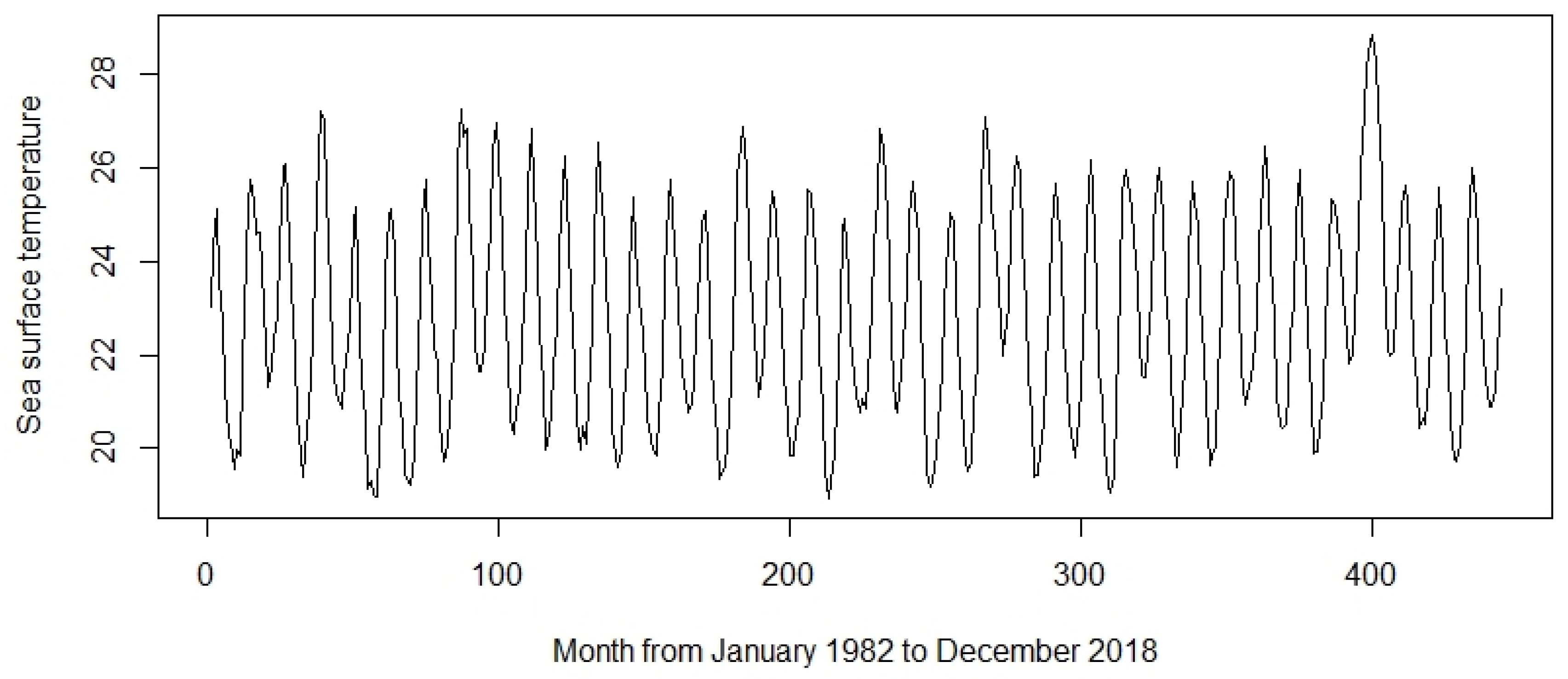
A functional time series is a sequence of functional objects that are dependent. For example, in Figure 1, a classical time series of monthly sea surface temperatures (in °C) from January 1982 to December 2018 is plotted. These sea surface temperatures were measured by Moore buoys in the ‘Niño region’. The functional versions of the same data points are represented in Figure 2. One functional observation represents the sea surface temperature for one year. From the $12\times 37$ data of the classical time series, we generate 37 observations of a functional time series that are observed each month. More generally, a functional time series $X_t\left(u\right)$, where $t=1,\dots ,N$ (N is the sample size of the functional time series) and $u\in [0,1]$ (where there are m points by functional observations we observe at the points $u_i$$i=1,\dots ,m$ from $[0,1]$) can be generated from a classical time series $x_t$ where $t=1,\dots ,N*m$, with m being the number of observations points. We have the relation $X_t\left(u_i\right)=x_{(t-1)\times m+i}$.

The functional time series must be stationary in order for our test to perform well. It is worth mentioning that stationarity for functional time series and stationarity for classical time series are quite different. For example, we could have a stationary functional time series from a classical time series that is not stationary. Mainly, it is the case when the classical time series has a seasonality over a period T, and we cut this series at these intervals of time.The classical time series appears non-stationary, but if we consider the data as functional observations, it can be stationary. Hence, our test provides a natural framework to test causality for classical non-stationary time series. The application of a traditional test and our procedure to the real dataset highlight this fact.

In Section 2, the definition of causality for functional stationary time series and an example in the autoregressive functional processes are introduced. In Section 3, we recall how we can estimate the dynamic FPCA and propose three algorithms for testing the non-causality including the dynamic FPCA-based testing procedure. We conclude this article with Section 4 and Section 5, which are developed to empirically analyze the testing procedure, and an application of the procedure to explain the relation between electricity demand and temperature in Australia.

2. Linear Causality with Two Functional Time Series

2.1. Definition

Let $\mathcal{H}$ be a separable Hilbert space, with its inner product $\langle ·,·\rangle$ and the norm associated $\parallel h\parallel =\sqrt{\langle h,h\rangle },\forall h\in \mathcal{H}$. We take $\mathcal{H}=L^2[0,1]$ for simplicity. Thereafter, for every functional time series ${\left\{Z_t\right\}}_{t\in \mathbb{Z}}$ valued in $\mathcal{H}$, we make the assumptions that $\mathbb{E}\left[\parallel Z_t{\parallel }^2\right]<+\infty$ and $\mathbb{E}\left[Z_t\right]=0$, $\forall t\in \mathbb{Z}$; moreover, we assume that ${\left\{Z_t\right\}}_{t\in \mathbb{Z}}$ is strongly stationary. Let us recall the two definitions: strongly and weakly stationary. We say that series of random functions $\left(Z_t\right)$ are strongly stationary if for any $h\in \mathbb{Z}$, $k\in \mathbb{N}$ and any sequence of indices $t_1,\dots ,t_k$, $(Z_{t_1},\dots ,Z_{t_k})$ and $(Z_{h+t_1},\dots ,Z_{h+t_k})$ are identically distributed. We say that ${\left\{Z_t\right\}}_{t\in \mathbb{Z}}$ is weakly stationary if for all t we have:

(i)

$Z_t$ verifies $\mathbb{E}\left[\parallel Z_t{\parallel }^2\right]<+\infty$,

(ii)

$\mathbb{E}{Z}_t=\mathbb{E}{Z}_0$,

(iii)

$\forall h\in \mathbb{Z},\forall (u,v)\in {\left[0,1\right]}^2$, we have $\mathrm{cov}(Z_{t+h}\left(u\right),Z_t\left(v\right))=\mathrm{cov}(Z_h\left(u\right),Z_0\left(v\right))$.

Let us introduce a key concept in functional data analysis about the second-order property of the process. To understand why this operator is a key concept, we recommend reading [19]. We define the operator of covariance ${\Gamma }_Z$ of the stationary functional time series $Z_t$ by:

$${\Gamma }_Z\left(U\right)=\mathbb{E}\left[\langle Z,U\rangle Z\right],\forall U\in \mathcal{H},$$

(1)

where we omit the index t of time, due to stationarity. It is well known that this operator is a self-adjoint, positive, nuclear operator.

Let $X_t$ and $Y_t$ be two stationary functional time series valued in $\mathcal{H}$. Let $U_t$ be the information accumulated since time $t-1$, and $U_t-X_t$ denote all this information without the series $X_t$. Define the predictive error series by

$${\epsilon }_t\left(Y\right|U)=Y_t-{\widehat{Y}}_t\left(U\right),$$

where ${\widehat{Y}}_t\left(U\right)$ is the best linear predictor of $Y_t$ using the information $U_t$. Then, we have the following definition.

Definition 1

(Causality). We say that X is causing Y if ${\Gamma }_{\epsilon \left(Y\right|U-X)}-{\Gamma }_{\epsilon \left(Y\right|U)}$ is a positive definite operator.

This definition is a natural extension of the idea of causality studied by Granger [5]. In fact, we replace the variance of the time series by the covariance operator of the functional time series. In addition, in order to compare covariance operator, we assume that a symmetric operator A is greater than a symmetric operator B if the difference $A-B$ is a positive definite operator. This is a theoretical definition because, in general, we do not have access to the information $U_t$, so we must be careful for the conclusions in practice.

2.2. An Example

Let ${\mathbb{X}}_t={(Y_t,X_t)}^{\prime }$ be an autoregressive process valued at $\mathcal{H}:=L^2[0,1]\times L^2[0,1]$ associated with $(\rho ,\epsilon )$, where $\rho$ is a linear operator of $\mathcal{H}$ and $\epsilon$ is a $\mathcal{H}$-strong white noise. For more information on the definition of autoregressive process valued in separable Hilbert space, see [3]. We have

$${\mathbb{X}}_t=\rho \left({\mathbb{X}}_{t-1}\right)+{\epsilon }_t.$$

(2)

We can rewrite the model as

$$\left\{\begin{array}{c}{Y}_t={\rho }_{11}\left(Y_{t-1}\right)+{\rho }_{12}\left(X_{t-1}\right)+{\epsilon }_{1t},\hfill \\ X_t={\rho }_{21}\left(Y_{t-1}\right)+{\rho }_{22}\left(X_{t-1}\right)+{\epsilon }_{2t},\hfill \end{array}\right.$$

with ${\rho }_{11}:={\left(\rho {\upharpoonright }_{L^2[0,1]\times 0}\right)}^{\left(1\right)}$, ${\rho }_{12}:={\left(\rho {\upharpoonright }_{0\times L^2[0,1]}\right)}^{\left(1\right)}$ and the same idea for ${\rho }_{21}$ and ${\rho }_{22}$. The symbol $f{\upharpoonright }_A$ stands for the restriction of the function f on the subset A of a definition set. The notation $F^{\left(1\right)}$ for an operator F, whose image is on a product space, means we take only the first component of the operator. According to the Definition 1, we say that $\left(X_t\right)$ does not linearly cause $\left(Y_t\right)$ if and only if ${\rho }_{12}=0$. In fact, if ${\rho }_{12}=0$, the two covariance operators of the definition are equals, and then the difference between the operators cannot be positively defined.

3. Testing Linear Causality

3.1. Dynamic FPCA

Hörmann et al. [17] have proposed a dynamic version of functional principal component analysis (FPCA) that is more efficient for functional time series than the traditional FPCA. As stated by [17] “classical static FPCs still can be consistently estimated, but, in contrast to the i.i.d. setup, they will not lead to an adequate dimension reduction technique”. In fact, the dynamic FPCs tend to recover the process better than the traditional FPCs. In this section, we recall briefly the practical aspects of this method. We consider a functional time series $(X_t:t\in \mathbb{Z})$ where $X_t$ takes values in $L^2[0,1]$. We assume here that $(X_t:t\in \mathbb{Z})$ is weakly stationary. We define the autocovariance kernels $c_h$ by

$$c_h(u,v)=\mathrm{cov}(X_h\left(u\right),X_0\left(v\right)),\forall u,v\in [0,1].$$

We denote $C_h$, $h\in \mathbb{Z}$ as the operator corresponding to the autocovariance kernels as $c_h$ and ${\widehat{C}}_h$ as the empirical counterpart of $C_h$ at lag h. We define the estimated spectral density operator at frequency $\theta$:

$${\widehat{\mathcal{F}}}_{\theta }=\sum _{\left|h\right|\le q}\left(1-\frac{\left|h\right|}{q}\right){\widehat{C}}_h{e}^{-ih\theta },0<q<n.$$

Then, we can estimate the m-th dynamic functional principal score by

$${\widehat{Y}}_{mt}=\sum _{l=-L}^L\langle X_{t-l},{\widehat{\varphi }}_{ml}\rangle ,m=1,\dots ,p\mathrm{and}t=L+1,\dots ,n-L,$$

where L is some integer and ${\widehat{\varphi }}_{ml}$ are the m-th estimated dynamic FPC filter coefficients coming from the fourier transform of the eigenfunction of ${\widehat{\mathcal{F}}}_{\theta }$.

3.2. Three Procedures for Testing the Causality

This first testing procedure is called F-causality (see Algorithm 1) and is explained in detail in [6]. We propose an enhanced procedure (see Algorithm 2) inspired by [18] and by [17] based on dynamic functional principal components. This is the second testing procedure. In this case, the number of dynamic functional principal components (d and $d^{\prime }$) can be chosen to explain a reasonable part of the variance (for example, $85\%$). This second procedure is called Dynamic-FPCA. We propose a last procedure, called the Classical test. This last procedure is based on differentiating the series, which are viewed as classical time series of period m.

Recall that we have

$$\begin{array}{ccc}{H}_0& :& \mathrm{No}\mathrm{causal}\mathrm{relation},\\ H_1& :& \mathrm{causal}\mathrm{relation},\end{array}$$

and in the case of FAR(1), this is equivalent to

$$\begin{array}{ccc}{H}_0& :& {\rho }_{12}=0\\ H_1& :& {\rho }_{12}\ne 0.\end{array}$$

We present the three procedures of testing non-causality under the form of the Algorithms 1–3. Algorithm 1 refers to first testing procedure (F-causality). The second one (Algorithm 2) is based on the scores of the dynamic functional principal components, and the second testing procedure (Dynamic-FPCA). The last one (Algorithm 3) refers to the classical testing procedure (Classical).

Algorithm 1 F-causality Test

(1) (Data) We have $(X_1,\dots ,X_n)$ and $(Y_1,\dots ,Y_n)$ (2) (Estimation of the parameters) We perform the estimation of $\rho$ according to the previous section. We separate the two different models, one estimation of $\rho$ without the $Y_i$ (nested model) and one that includes them (pooled model). (3) (Estimation of the errors) ${\epsilon }_1$ is then estimated in the different models for $t=2,\dots ,n$, by $$\left\{\begin{array}{c}{\widehat{\epsilon }}_t^1=Y_t-{\widehat{\rho }}_{11}\left(Y_{t-1}\right)+{\widehat{\rho }}_{12}\left(X_{t-1}\right),(\mathrm{pooled}\mathrm{model}),\hfill \\ {\widehat{\epsilon }}_t^2=Y_t-{\widehat{\rho }}_{11}\left(Y_{t-1}\right),(\mathrm{nested}\mathrm{model}).\hfill \end{array}\right.$$ (4) (Test the equality of operators based on the errors) We perform the proposed test of Zhang and Shao [16] on the equality of the covariance operators of the estimated errors.

Algorithm 2 Dynamic-FPCA Test

(1) (Data) We have $(X_1,\dots ,X_n)$ and $(Y_1,\dots ,Y_n)$. (2) (Parameters) Choose L and q defined in Section 3.1. (3) (Dynamic FPCA) Compute the first d and $d^{\prime }$ dynamic FPCA scores for the two functional time series. (4) Use a multivariate test on the scores to conclude. For instance, (a) Model the scores by a VAR model. (b) Apply a Wald test on the scores.

Algorithm 3 Classical Test

(1) (Data) We have $(X_1,\dots ,X_n)$ and $(Y_1,\dots ,Y_n)$, and each curve has m points. (2) (time series) We obtain two “classical” time series $(x_1,\dots ,x_{m*n})$ and $(y_1,\dots ,y_{m*n})$ by not viewing them as functional time series. (3) (Differencing) Due to the potentially non-stationarity of these classical time series, we use the differencing technique of period m. (4) Use a multivariate test to conclude.

4. Empirical Analysis

4.1. Design of the Experiments

A simulation study was developed to check the performance of the three procedures. We used R software, namely package “fda” [20], “far” [21] and “freqdom.fda”. To verify the results of our test under the Null and the alternatives, we simulated different scenarios. We used the packages “far” in order to simulate functional time series and to estimate the parameters of the models, the package “fda” to perform the test of equality of covariance and the package “freqdom.fda” to compute the dynamic FPCA scores. Under the null, we used three independent functional time series and one model computed with the “far” package (see “Null 1”). Under the alternative of causality, we tested five different scenarios. We simulated with $\rho$ on a sinusoidal basis that approximates the Hilbert space $\mathcal{H}$. In fact, we used the function “theoretical.coef” (package “far”) to obtain the parameters used internaly by the function “simul.farx” (package “far”) to make the simulation.

Table 1. Six scenario for the simulations of $\rho$.

Scenario	$\mathit{\rho }$	Dim X and Y
Null 1	$\left(\begin{array}{ccccc}0.45& 0.00& 0.00& 0.00& 0.00\\ 0.00& 0.3& 0.00& 0.00& 0.00\\ 0.00& 0.0& 0.34& 0.00& 0.00\\ 0.00& 0.0& 0.00& 0.45& 0.00\\ 0.00& 0.00& 0.00& 0.00& 0.40\end{array}\right)$	3, 2
1	$\left(\begin{array}{ccccc}0.45& 0.00& 0.00& 0.002& 0.001\\ 0.00& 0.3& 0.00& 0.001& 0.002\\ 0.00& 0.0& 0.34& 0.00& 0.00\\ 0.00& 0.0& 0.00& 0.45& 0.00\\ 0.00& 0.00& 0.00& 0.00& 0.40\end{array}\right)$	3, 2
2	$\left(\begin{array}{ccccc}0.45& 0.00& 0.00& 0.02& 0.01\\ 0.00& 0.3& 0.00& 0.01& 0.02\\ 0.00& 0.0& 0.34& 0.00& 0.00\\ 0.00& 0.0& 0.00& 0.45& 0.00\\ 0.00& 0.00& 0.00& 0.00& 0.40\end{array}\right)$	3, 2
3	$\left(\begin{array}{cccc}0.45& 0.00& 0.00& 0.50\\ 0.00& 0.3& 0.00& 0.00\\ 0.00& 0.0& 0.34& 0.00\\ 0.00& 0.0& 0.00& 0.45\end{array}\right)$	3, 1
4	$\left(\begin{array}{cccc}0.15& 0.00& 0.00& 0.40\\ 0.00& 0.10& 0.00& 0.20\\ 0.00& 0.00& 0.10& 0.20\\ 0.00& 0.00& 0.00& 0.45\end{array}\right)$	3, 1
5	$\left(\begin{array}{cccc}0.25& 0.00& 0.00& 0.40\\ 0.00& 0.10& 0.00& 0.00\\ 0.00& 0.0& 0.10& 0.00\\ 0.00& 0.00& 0.00& 0.45\end{array}\right)$	3, 1

presents the different forms for $\rho$.

The first scenario “Null 1” is used in the last line (line 4) of

Table 2. Nominal Level 0.05.

		Fcausality Test	DynamicFPCA Test			Classical Test
Model	N	K Optimal	nd			p
			1	2	3	1	2	3	4	5	6
1	100	0.047	0.057	0.06	0.074	0.537	0.237	0.043	0.038	0.014	0.009
	200	0.076	0.062	0.059	0.068	0.523	0.229	0.05	0.034	0.011	0.008
2	100	0.054	0.054	0.06	0.068	0.537	0.243	0.058	0.038	0.016	0.011
	200	0.078	0.064	0.057	0.061	0.514	0.216	0.057	0.036	0.02	0.012
3	100	0.052	0.059	0.054	0.063	0.54	0.257	0.052	0.039	0.022	0.012
	200	0.099	0.061	0.06	0.063	0.532	0.244	0.061	0.04	0.019	0.011
4	100	0.041	0.048	0.072	0.002	0.538	0.217	0.062	0.102	0.09	0.086
	200	0.055	0.055	0.071	0.001	0.539	0.236	0.07	0.101	0.088	0.083

of the level. Here, we represent the space $\mathcal{H}$ by the space $H_m\times H_m^{\prime }$. $H_m$ is the space of $Y_t$ and $H_m^{\prime }$ for $X_t$. Then, it can have more than two lines to represent $\rho$, depending on the dimension of approximations of the two spaces $H_m$ and $H_m^{\prime }$. For example, if we take $dim\left(H_m\right)=3$ and $dim\left(H_m^{\prime }\right)=2$ (as in the first scenario) with a basis with two components, then in the case of scenario 1, we have the following approximations:

$${\rho }_{11}=\left(\begin{array}{ccc}0.45& 0.00& 0.00\\ 0.00& 0.3& 0.00\\ 0.00& 0.00& 0.34\end{array}\right),{\rho }_{12}=\left(\begin{array}{cc}0.002& 0.001\\ 0.001& 0.002\\ 0.00& 0.00\end{array}\right),$$

$${\rho }_{21}=\left(\begin{array}{ccc}0.00& 0.00& 0.00\\ 0.00& 0.00& 0.00\end{array}\right),{\rho }_{22}=\left(\begin{array}{cc}0.45& 0.00\\ 0.00& 0.40\end{array}\right).$$

We use different values for $n=100,200$, with the parameter $ncv=20,40$ and $m=50$. n is the sample size, $ncv$ the number used for the cross validation in the model $FAR\left(1\right)$ and m is the number of discretization points used for one observation of the functional time series. The level of significance that was studied was $\alpha =0.05$. The two parameters L and q of the Dynamic-FPCA algorithm were chosen according to the freqdom.fda package initializations with $q=30$ and L as the minimum between the maximum possibilities and 60 (to avoid high calcuation time). For the analysis of d and $d^{\prime }$, we chose to give the same value $d=d^{\prime }$ for the sake of simplicity.

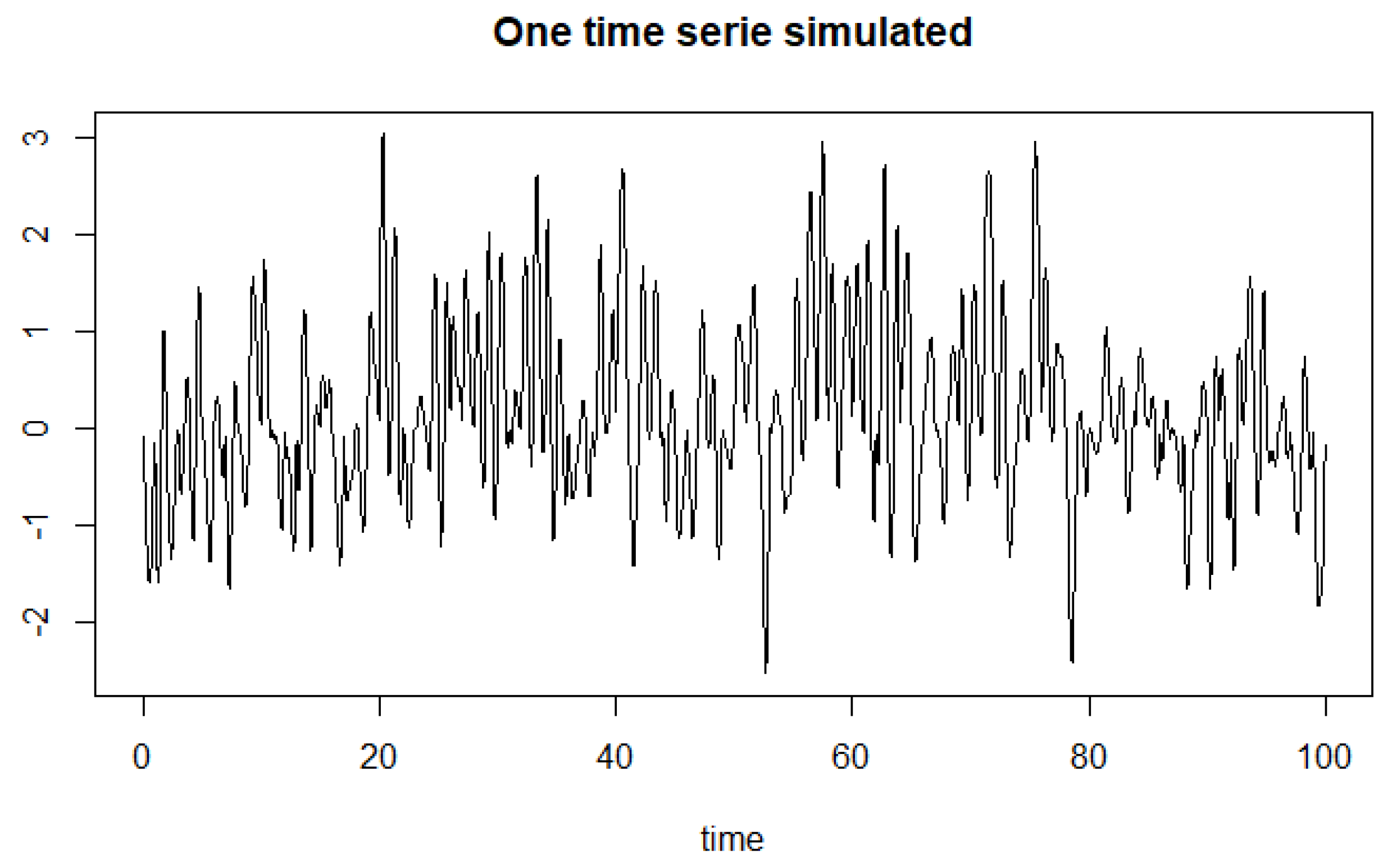
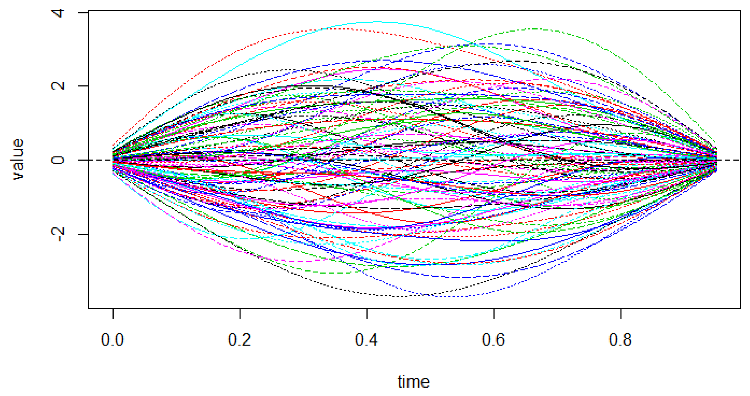
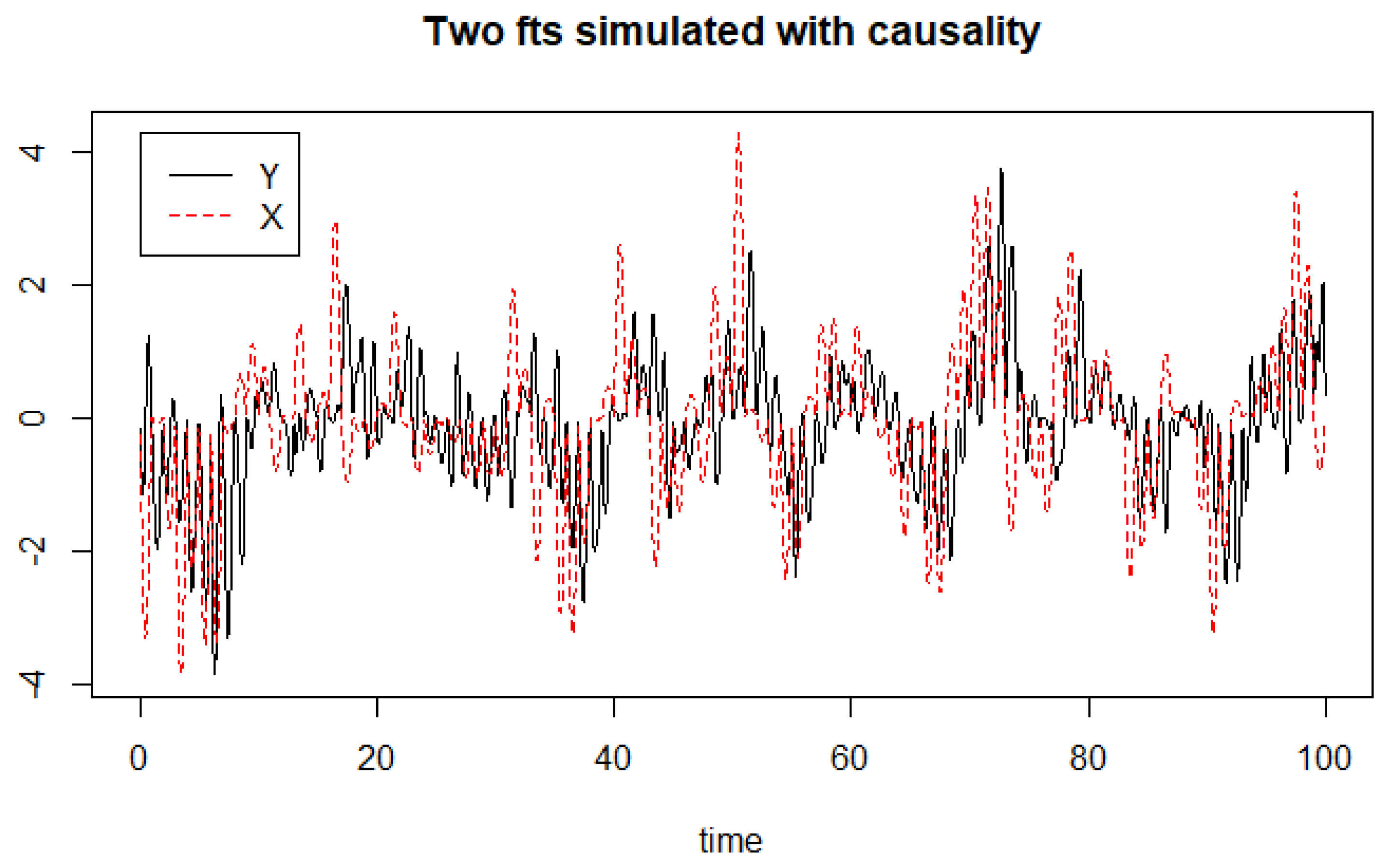
In order to have an idea of what we are manipulating, we made some plots of different time series; see Figure 3, Figure 4 and Figure 5. Figure 3 represents the whole trajectory of a functional time series simulated with sample size of 100. Figure 4 is the same as Figure 3 but we bring back the sequence series to the same time domain. Figure 5 plots the whole trajectory of two functional time series, which are in a causal relation.

4.2. Results

We present the type I error (power, respectively) in Table 2 (

Table 3. Power on five different models.

		Fcausality Test						DynamicFPCA Test			Classical Test
Model	N	K						nd			p
		1	2	3	4	5	6	1	2	3	1	2	3	4	5	6
1	100	0.761	0.918	0.865	0.735	0.489	0.214	0.069	0.153	0.004	0.552	0.231	0.073	0.1	0.09	0.086
	200	0.891	0.998	0.989	0.973	0.914	0.82	0.096	0.271	0.003	0.558	0.266	0.081	0.107	0.083	0.091
2	100	0.779	0.924	0.888	0.756	0.509	0.242	0.18	0.925	0.741	0.541	0.26	0.074	0.109	0.091	0.093
	200	0.895	0.996	0.992	0.972	0.915	0.826	0.287	0.999	0.99	0.564	0.314	0.082	0.126	0.093	0.09
3	100	0.733	0.907	0.857	0.75	0.487	0.241	0.988	0.987	0.98	0.665	0.223	0.371	0.434	0.472	0.487
	200	0.858	0.99	0.989	0.957	0.9	0.788	0.997	0.999	0.999	0.668	0.383	0.419	0.453	0.495	0.495
4	100	0.696	0.647	0.518	0.344	0.133	0.062	1	0.999	1	0.95	0.812	0.629	0.792	0.793	0.779
	200	0.949	0.939	0.917	0.779	0.507	0.303	1	1	1	0.993	0.989	0.963	0.982	0.975	0.967
5	100	0.662	0.727	0.566	0.368	0.15	0.071	0.971	0.96	0.93	0.677	0.124	0.293	0.385	0.424	0.458
	200	0.886	0.954	0.916	0.793	0.539	0.321	0.996	0.997	0.994	0.653	0.232	0.33	0.422	0.455	0.478

, respectively) for each different considered scenario. We make a replication of order 1000 for each scenario. Then, we count the number of rejections of the Null hypothesis, which in the case of a true Null hypothesis gives an approximation of the type I error and in the case of false Null hypothesis gives an approximation of the power of the test (which is $1-\beta$ where $\beta$ is the type II error).

In Table 2, we see that the nominal level $0.05$ is very well respected for the F-causality and Dynamic-FPCA tests and for different values of n. The parameter p of the classical test has to be well tuned, and there are many variations for this parameter. However, for $p=3$ and only its value in the different simulation setup, the classical test reaches the nominal level correctly.

In Table 3, we perform the test for the different scenarios with parameters $n=100$ or 200, $m=50$ and $K=1$ to 6. We observe, in general, that the power is sufficiently high for the five different models. The sample size plays a role in the power. Higher is the sample size, the better is the power of the test. With $n=200$, the power is sufficient. We can also see the influence of the parameter K. We also note that if K is badly selected, then there can be a lack of power, as we can see in model 3, for example.

4.3. Comparison of the Three Tests

Since the nominal level is well respected for the two first tests, it seems that the second test Dynamic-FPCA is more powerful than the two other tests in all the scenarios except for model 1. We can explain this by observing that the Dynamic-FPCA captures the properties of functional time series more, as shown in [17]. To understand the fact that model 1 is better for the F-causality test, we can say the departure from the null hypothesis is weak, as ${\rho }_{12}$ is nearly zero.

As the classical test does not reach the level of significance, and the Dynamic-FPCA seems more powerful than the F-causality test, we recommend that the Dynamic FPCA test is performed.

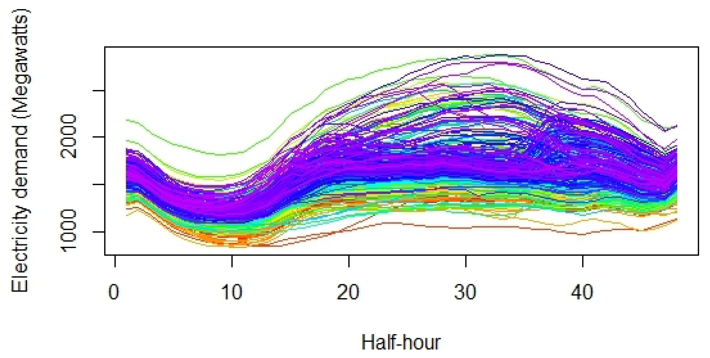
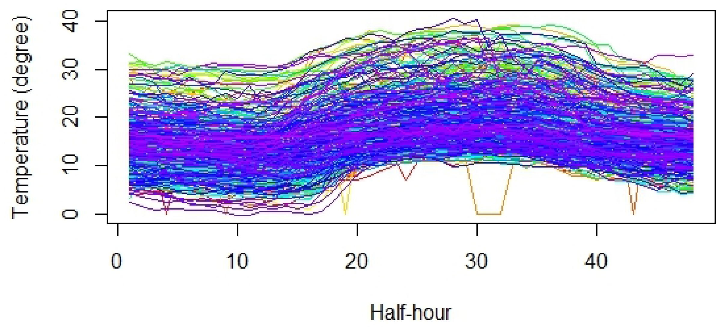
5. Real Data Illustration

The dataset we used is available in the R package “fds” [22] and is already studied in [23]. The article [23] deals with the electricity demands and the temperature in Adelaide. This dataset consists of half-hourly electricity demands in Adelaide and temperatures measured at the Adelaide airport from Sunday to Saturday between 6 July 1997 and 31 March 2007 (see Figure 6 for the electricity demand on Thursday and Figure 7 for the temperature on Thursday).

We wanted to test the causal relation between these two variables: the electricity demands and the temperatures. To do so, we used the three algorithms. As in article [23], we found a dependency between this two variables. Everyday, the temperatures in Adelaide impact the electricity demands in this city.

5.1. Results of F-Causality Algorithm

In order to test the causality between the electricity demands and the measured temperatures based on F-causality, some parameters need to be defined. Hence, the ncv was set to 100, and the number of replication (sample size) was set to 508. A generic test was performed between all days for the causality testing. For each test, a couple of results are calculated by finding the optimal K value, and results of the method are included in

Table 4. F-causality tests between temperature and electricity demand with an optimal parameter.

K Optimal	Monday	Tuesday	Wednesday	Thursday	Friday	Saturday	Sunday
Monday	1	1	1	1	1	1	1
	True	False	False	False	False	False	True
Tuesday	1	1	1	1	1	1	1
	False	False	False	False	False	False	False
Wednesday	1	1	1	1	1	1	1
	False	False	False	False	False	False	False
Thursday	1	1	1	1	1	1	1
	False	False	False	True	True	True	False
Friday	1	1	1	1	1	1	1
	False	False	False	False	True	True	False
Saturday	1	1	1	1	1	1	1
	False	False	False	False	False	True	False
Sunday	1	1	1	1	1	1	1
	True	False	False	False	False	False	True

. The line represents the electricity demand each day, and the column represents the temperature measured in the airport. Table 4 reports the optimal K value and causality result (“True” or “False”) for each couple. From both tables, we can clearly observe that with the optimal parameter method, the temperature affects the daily electricity demand, except on Tuesday and Wednesday. Moreover, it is also observed that the temperature on a given day may cause the electricity demand another day, which is explained by a similarity of temperatures.

5.2. Results of the Dynamic FPCA Algorithm

To perform the dynamic FPCA causality test, the same parameters as in F-causality are set. Moreover, in each couple of tests, the causality is calculated with different values of d parameter 1, 2 and 3, and results are presented in

Table 5. Dynamic FPCA test between temperature and electricity demand.We highligth the diagonal in red.

	Monday	Tuesday	Wednesday	Thursday	Friday	Saturday	Sunday
Monday	95%	61%	13%	30%	65%	96%	44%
	99%	99%	99%	99%	99%	99%	99%
	99%	99%	99%	99%	99%	99%	99%
Tuesday	96%	95%	84%	33%	66%	88%	18%
	99%	99%	99%	99%	99%	99%	99%
	99%	99%	99%	99%	99%	99%	99%
Wednesday	58%	54%	98%	82%	39%	92%	51%
	99%	99%	99%	99%	99%	99%	99%
	99%	99%	99%	99%	99%	99%	99%
Thursday	39%	20%	77%	99%	58%	88%	82%
	99%	99%	99%	99%	99%	99%	99%
	99%	99%	99%	99%	99%	99%	99%
Friday	54%	73%	94%	6%	98%	63%	99%
	99%	99%	99%	99%	99%	99%	99%
	99%	99%	99%	99%	99%	99%	99%
Saturday	54%	85%	96%	73%	88%	97%	99%
	99%	99%	99%	99%	99%	99%	99%
	99%	99%	99%	99%	99%	99%	99%
Sunday	54%	65%	61%	86%	63%	94%	89%
	99%	99%	99%	99%	99%	99%	99%
	99%	99%	99%	99%	99%	99%	99%

.

Table 5 reports the causality result in terms of percentage for each couple. Firstly, the obtained results when d is set to 2 and 3 are not discriminative since they show high causality for all couples. Secondly, it can be noticed that the temperature causes the electricity demand each day. Furthermore, it is also observed that the temperature on a given day may cause the electricity demand another day.

5.3. Results of the Classical Algorithm

In order to compare, we also performed the classical test (

Table 6. Classical tests between temperature and electricity demands. We highligth the diagonal in red.

$\mathit{p}=3$	Monday	Tuesday	Wednesday	Thursday	Friday	Saturday	Sunday
Monday	$3.88\times {10}^{-15}$	<$2.2\times {10}^{-16}$	$7.757\times {10}^{-10}$	$1.964\times {10}^{-7}$	0.03575	0.5818	0.516
Tuesday	0.0028	<$2.2\times {10}^{-16}$	<$2.2\times {10}^{-16}$	$1.1527\times {10}^{-12}$	0.003014	0.3427	0.188
Wednesday	0.0383	0.001607	<$2.2\times {10}^{-16}$	<$2.2\times {10}^{-16}$	0.0002952	0.9729	0.691
Thursday	0.62	0.7831	0.5706	<$2.2\times {10}^{-16}$	<$2.2\times {10}^{-16}$	$4.6\times {10}^{-12}$	0.172
Friday	0.107	0.3103	0.4036	0.03976	<$2.2\times {10}^{-16}$	<$2.2\times {10}^{-16}$	0.0221
Saturday	0.032	0.2931	0.1128	0.02072	$3.066\times {10}^{-12}$	<$2.2\times {10}^{-16}$	$5.83\times {10}^{-6}$
Sunday	$1.5\times {10}^{-10}$	$6.873\times {10}^{-5}$	0.2707	0.1951	0.01001	$1.027\times {10}^{-5}$	$7.88\times {10}^{-07}$

) with the p-values. There is a major drawback to performing a classical test, namely non-stationarity. In fact, the functional analysis allows us to perform the test directly on the functional series, which can be directly seen as stationary functional series. In the classical setting, we must differentiate the fourteen series at lag 48 to remove the seasonal components. We chose to differentiate the series at lag 48 because of the recording of the series. In fact, the series is recorded every half hour in a day. Therefore, we chose to differentiate at lag $2\times 24$. Furthermore, we chose to fix p at 3, as it seems to perform at this value in the simulations. The same conclusion for each day holds for the classical test as the Dynamic-FPCA test.

6. Conclusions

Causality is a hard notion due to the lack of universal definition. One notion of linear causality for functional data was proposed and studied. We have proposed three statistical procedures to test this concept in a special case, i.e., the autoregressive model of order 1. A mathematical study of the behavior of the testing procedures would be an interesting future work. Extensions to more general models will be also considered in future work. The performance of the proposed testing procedures shows good behavior in simulations. The simulation study shows different behaviors between classical test, F-causality test and the Dynamic-FPCA test. An application to the electricity demands and the temperature is studied in detail. Finally, we can conclude that the dynamic FPCA algorithm is more suitable for the causality test due to its effectiveness to measure the causality with precision. Possible alternatives to the test of Zhang and Shao would be to perform a global F-test as in [24] or to test the effect of the variable X on errors as [25]. Another possible extension is to study the link between the shape through the phase and amplitude variation in functional data [2] and causality.

References

- Ramsay, J.O.; Silverman, B.W. Functional Data Analysis; Wiley Online Library: New York, NY, USA, 2006. [Google Scholar]
- Srivastava, A.; Klassen, E.P. Functional and Shape Data Analysis; Springer: New York, NY, USA, 2016. [Google Scholar] [CrossRef] [Green Version]
- Bosq, D. Linear Processes in Function Spaces:Theory and Applications; Lecture Notes in Statistics; Springer: New York, NY, USA, 2000; Volume 149, pp. xiv+283. [Google Scholar] [CrossRef]
- Horváth, L.; Kokoszka, P. Inference for Functional Data with Applications; Springer: New York, NY, USA, 2012; Volume 200. [Google Scholar]
- Granger, C.W.J. Investigating Causal Relations by Econometric Models and Cross-spectral Methods. Econometrica 1969, 37, 424–438. [Google Scholar] [CrossRef]
- Saumard, M. Linear causality in the sense of Granger with stationary functional time series. In Functional Statistics and Related Fields; Aneiros, G., Bongiorno, E.G., Cao, R., Vieu, P., Eds.; Springer International Publishing: Cham, Switzerland, 2017; pp. 225–231. [Google Scholar]
- Elmezouar, Z.C. Functional Causality between Oil Prices and GDP Based on Big Data. Comput. Mater. Contin. 2020, 63, 593–604. [Google Scholar] [CrossRef]
- Sancetta, A. Intraday End-of-Day Volume Prediction. J. Financ. Econom. 2019, nbz019. [Google Scholar] [CrossRef]
- Wiener, N. The theory of prediction. Mod. Math. Eng. 1956, 1, 125–139. [Google Scholar]
- Gourieroux, C.; Monfort, A. Time Series and Dynamic Models; Cambridge University Press: Cambridge, MA, USA, 1997; Volume 3. [Google Scholar]
- Dufour, J.M.; Taamouti, A. Short and long run causality measures: Theory and inference. J. Econom. 2010, 154, 42–58. [Google Scholar] [CrossRef] [Green Version]
- Geweke, J. Measurement of linear dependence and feedback between multiple time series. J. Am. Stat. Assoc. 1982, 77, 304–313. [Google Scholar] [CrossRef]
- Taamouti, A.; Bouezmarni, T.; El Ghouch, A. Nonparametric estimation and inference for conditional density based Granger causality measures. J. Econom. 2014, 180, 251–264. [Google Scholar] [CrossRef] [Green Version]
- Pearl, J.; Verma, T.S. A theory of inferred causation. Stud. Log. Found. Math. 1995, 134, 789–811. [Google Scholar]
- Hörmann, S.; Kokoszka, P. Weakly dependent functional data. Ann. Stat. 2010, 38, 1845–1884. [Google Scholar] [CrossRef] [Green Version]
- Zhang, X.; Shao, X. Two sample inference for the second-order property of temporally dependent functional data. Bernoulli 2015, 21, 909–929. [Google Scholar] [CrossRef]
- Hörmann, S.; Kidziński, Ł.; Hallin, M. Dynamic functional principal components. J. R. Stat. Soc. Ser. B Stat. Methodol. 2015, 77, 319–348. [Google Scholar] [CrossRef]
- Aue, A.; Norinho, D.D.; Hörmann, S. On the prediction of stationary functional time series. J. Am. Stat. Assoc. 2015, 110, 378–392. [Google Scholar] [CrossRef] [Green Version]
- Hsing, T.; Eubank, R. Theoretical Foundations of Functional Data Analysis, with an Introduction to Linear Operators; John Wiley & Sons: West Sussex, UK, 2015. [Google Scholar]
- Ramsay, J.O.; Wickham, H.; Graves, S.; Hooker, G. fda: Functional Data Analysis. R Package Version 2.4.7. 2017. Available online: http://CRAN.R-project.org/package=fda (accessed on 7 June 2021).
- Damon, J.; Guillas, S. far: Modelization for Functional AutoRegressive Processes. R Package Version 0.6-5. 2015. Available online: https://mran.microsoft.com/snapshot/2015-11-17/web/packages/far/index.html (accessed on 7 June 2021).
- Shang, H.L.; Hyndman, R.J. fds: Functional Data Sets. R Package Version 1.7. 2013. Available online: https://cran.r-project.org/package=fds (accessed on 7 June 2021).
- Magnano, L.; Boland, J.; Hyndman, R. Generation of symthetic sequences of halfhourly temperature. Environmetrics 2008, 19, 818–835. [Google Scholar] [CrossRef]
- Shen, Q.; Faraway, J. An F test for linear models with functional responses. Stat. Sin. 2004, 14, 1239–1257. [Google Scholar]
- Patilea, V.; Sánchez-Sellero, C.; Saumard, M. Testing the predictor effect on a functional response. J. Am. Stat. Assoc. 2016, 111, 1684–1695. [Google Scholar] [CrossRef]
Figure 1.
Monthly sea surface temperatures.
Figure 2.
Monthly sea surface temperatures as functional observations by year.
Figure 3.
One trajectory.
Figure 4.
One trajectory on the same time domain.
Figure 5.
The trajectory of two functional time series with a causal relation.
Figure 6.
Electricity demand in Adelaide for Thursday.
Figure 7.
Temperature in Adelaide for Thursday.