Robustness and Sensitivity Tuning of the Kalman Filter for Speech Enhancement

Abstract

Inaccurate estimates of the linear prediction coefficient (LPC) and noise variance introduce bias in Kalman filter (KF) gain and degrade speech enhancement performance. The existing methods propose a tuning of the biased Kalman gain, particularly in stationary noise conditions. This paper introduces a tuning of the KF gain for speech enhancement in real-life noise conditions. First, we estimate noise from each noisy speech frame using a speech presence probability (SPP) method to compute the noise variance. Then, we construct a whitening filter (with its coefficients computed from the estimated noise) to pre-whiten each noisy speech frame prior to computing the speech LPC parameters. We then construct the KF with the estimated parameters, where the robustness metric offsets the bias in KF gain during speech absence of noisy speech to that of the sensitivity metric during speech presence to achieve better noise reduction. The noise variance and the speech model parameters are adopted as a speech activity detector. The reduced-biased Kalman gain enables the KF to minimize the noise effect significantly, yielding the enhanced speech. Objective and subjective scores on the NOIZEUS corpus demonstrate that the enhanced speech produced by the proposed method exhibits higher quality and intelligibility than some benchmark methods.

1. Introduction

The main objective of a speech enhancement algorithm (SEA) is to improve the quality and intelligibility of noisy speech [1]. It can be achieved by eliminating the embedded noise from a noisy speech signal without distorting the speech. Many speech processing systems, such as speech communication systems, hearing aid devices, and speech recognition systems, somehow rely upon the enhancement of noisy speech. Various SEAs, namely spectral subtraction (SS) [2,3,4,5], Wiener Filter (WF) [6,7,8], minimum mean square error (MMSE) [9,10,11], Kalman filter (KF) [12], augmented KF (AKF) [13], and deep neural networks (DNNs) [14,15,16], have been introduced over the decades. This paper focuses on KF-based speech enhancement in real-life noise conditions.

The Kalman filter (KF) was first used for speech enhancement by Paliwal and Basu [12]. In KF, a speech signal is represented by an autoregressive (AR) process, whose parameters comprise the linear prediction coefficients (LPCs) and prediction error variance. The LPC parameters and noise variance are used to construct the KF recursion equations. KF gives a linear MMSE estimate of the current state of the clean speech given the observed noisy speech for each sample within a frame. Therefore, the performance of KF-based SEA largely depends on how accurately the LPC parameters and noise variance are estimated. Experiments demonstrated that the KF shows excellent performance in stationary white Gaussian noise (WGN) conditions when the LPC parameters are estimated from clean speech [12]. On the contrary, the LPC parameters and the noise variance directly computed from the noisy speech would be inaccurate and unreliable, which leads to performance degradation.

In [13], Gibson et al. introduced an augmented KF (AKF) to enhance colored noise-corrupted speech. In this SEA, both the clean speech and noise signal are represented by two AR processes. The speech and noise LPC parameters are incorporated in an augmented matrix form to construct the recursive equations of AKF. In [13], the AKF processes the colored noise-corrupted speech iteratively (usually 3–4 iterations) to eliminate the noise, yielding the enhanced speech. Specifically, the LPC parameters for the current frame are computed from the corresponding filtered speech frame of the previous iteration by AKF. Although the enhanced speech of the AKF demonstrates an improvement in signal-to-noise ratio (SNR), it suffers from musical noise and speech distortion. Therefore, this method [13] does not adequately address the inaccurate LPC parameter estimation issue in practice.

In [17], So and Paliwal proposed a modulation-domain KF (MDKF) for speech enhancement. It was claimed that the modulation domain is able to better model the long-term correlation of speech information than that of time domain speech. It was shown that the MDKF exhibits better objective scores than time-domain KF (TDKF), particularly in the oracle case (LPC parameters are computed from clean speech). However, clean speech is unobserved in practice. For practical applications, they incorporated a traditional MMSE-STSA [9] with MDKF for speech enhancement. Specifically, the MMSE-STSA has been used to pre-filter the noisy speech in the acoustic domain. Then, the pre-filtered speech is transformed in the modulation domain prior to computing the LPC parameters. Therefore, they do not adequately address LPC parameter estimation directly from the noisy speech in the modulation domain. Technically, the characteristics of the speech signal in the acoustic domain are entirely different than that of it in modulation domain. Due to this limitation, it is quite difficult to assess the performance of MDKF for speech enhancement in practice. Roy et al. introduced a sub-band (SB) iterative KF (SBIT-KF)-based SEA [18]. This method enhances only the high-frequency sub-bands (SBs) using iterative KF among the 16 decomposed SBs of noisy speech for a given utterance, with the assumption that the impact of noise in low-frequency SBs is negligible. However, the low-frequency SBs can also be affected by noise, typically when operating in real-life noise conditions. As demonstrated in [13], the SBIT-KF [18] also suffers from speech distortion due to the iterative processing of noisy speech by KF.

In [19], Saha et al. propose a robustness metric and a sensitivity metric for tuning the biased KF gain for instrument engineering applications. Later on, So et al. applied the tuning of KF gain for speech enhancement in the WGN condition [20,21]. Specifically, the enhanced speech (for each sample within a noisy speech frame) is given by recursively averaging the observed noisy speech and the predicted speech weighted by a scalar KF gain [20]. However, the inaccurate estimates of LPC parameters introduce bias in the KF gain, resulting in leaking a significant residual noise in the enhanced speech. In [20], a robustness metric is used to offset the bias in KF gain for speech enhancement. However, So et al. further showed that the robustness metric strongly suppresses the KF gain in speech regions, resulting in distorted speech [21]. In [21], a sensitivity metric was used to offset the bias in KF gain, which produced less distorted speech. In [22], George et al. propose a robustness metric-based tuning of the AKF (AKF-RMBT) for enhancing colored noise-corrupted speech. As in [20], the adjusted AKF gain is underestimated in speech regions, resulting in distorted speech.

The existing KF methods [20,21] address tuning of biased Kalman gain in the WGN condition with the prior assumption that the impact of WGN on LPCs is negligible. Though the AKF method [22] performs tuning of biased gain in colored noise conditions, it still produced distorted speech. In this paper, we address the tuning of KF gain for speech enhancement in real-life noise conditions. For this purpose, we estimate noise from each noisy speech frame using an SPP-based method to compute the noise variance. To minimize bias in the LPC parameters, we compute them from pre-whitened speech. Then, KF is constructed with the estimated parameters. To achieve better noise reduction, the robustness metric is applied to offset the bias in Kalman gain when there is speech absent to that of the sensitivity metric during speech presence of the noisy speech. We also adopt the noise variance and the AR model parameters as a speech activity detector. The reduced-biased KF gain exhibits better suppression of noise in the enhanced speech. The performance of the proposed SEA is compared against some benchmark methods using objective and subjective testing.

The structure of this paper is as follows: Section 2 describes the KF for speech enhancement, including the paradigm shift of the KF recursive equations, the impact of biased KF gain on KF-based speech enhancement in WGN and real-life noise conditions. In Section 3, we describe the proposed SEA, which includes the proposed parameter estimation and the proposed Kalman gain tuning algorithm. Following this, Section 4 describes the experimental setup in terms of speech corpus, objective and subjective evaluation metrics, and specifications of competitive SEAs. The experimental results are then presented in Section 5. Finally, Section 6 gives some concluding remarks.

2. Kalman Filter for Speech Enhancement

Assuming that the noise, $v\left(n\right)$, is additive and uncorrelated with the clean speech, $s\left(n\right)$, at sample n, the noisy speech, $y\left(n\right)$, can be represented as:

$$\begin{array}{cc}\hfill y\left(n\right)& =s\left(n\right)+v\left(n\right).\hfill \end{array}$$

(1)

The clean speech, $s\left(n\right)$, can be represented by a $p^{th}$ order autoregressive (AR) model as ([23], Chapter 8):

$$\begin{array}{cc}\hfill s\left(n\right)& =-\sum _{i=1}^p{a}_{i}s(n-i)+w\left(n\right),\hfill \end{array}$$

(2)

where $\{a_i;i=1,2,\dots ,p\}$ are the LPCs and $w\left(n\right)$ is assumed to be a white noise with zero mean and variance ${\sigma }_w^2$.

Equations (1) and (2) can be used to form the following state-space model (SSM) of the KF (where the bold variables denote vector/matrix quantities, as opposed to unbolded variables for scalar quantities):

$$\begin{array}{c}\hfill \mathit{x}\left(n\right)=\mathsf{\Phi }\mathit{x}(n-1)+\mathit{d}w\left(n\right),\end{array}$$

(3)

$$\begin{array}{c}\hfill y\left(n\right)={\mathit{c}}^{\top }\mathit{x}\left(n\right)+v\left(n\right).\end{array}$$

(4)

In the above SSM:

• $\mathit{x}\left(n\right)$ is a $p\times 1$ state vector at sample n, given by:

  $$\mathit{x}\left(n\right)={[s\left(n\right) s(n-1) \dots s(n-p+1)]}^{\top },$$

  (5)
• $\mathsf{\Phi }$ is a $p\times p$ state transition matrix, represented as:

  $$\mathsf{\Phi }=\left[\begin{array}{ccccc}-a_1& -a_2& \dots & -a_{p-1}& -a_p\\ 1& 0& \dots & 0& 0\\ 0& 1& \dots & 0& 0\\ ⋮& ⋮& \ddots & ⋮& ⋮\\ 0& 0& \dots & 1& 0\end{array}\right],$$

  (6)
• $\mathit{d}$ and $\mathit{c}$ are the $p\times 1$ measurement vectors for the excitation noise and observation, written as:

  $$\mathit{d}=\mathit{c}={\left[\begin{array}{cccc}1& 0& \dots & 0\end{array}\right]}^T,$$
• $y\left(n\right)$ is the observed noisy speech at sample n.

During the operation of KF, the noisy speech, $y\left(n\right)$, is windowed into non-overlapped and short (e.g., 20 ms) frames. For a particular frame, the KF recursively computes an unbiased linear MMSE estimate, $\widehat{\mathit{x}}\left(n\right|n)$, of the state vector, $\mathit{x}\left(n\right)$, given the observed noisy speech up to sample n, i.e., $y\left(1\right),y\left(2\right),\dots ,y\left(n\right)$, using the following equations [12]:

$$\begin{array}{cc}\hfill & \widehat{\mathit{x}}\left(n\right|n-1)=\mathsf{\Phi }\widehat{\mathit{x}}(n-1|n-1),\hfill \end{array}$$

(7)

$$\begin{array}{cc}\hfill & \mathsf{\Psi }\left(n\right|n-1)=\mathsf{\Phi }\mathsf{\Psi }(n-1|n-1){\mathsf{\Phi }}^{\top }+{\sigma }_w^2\mathit{d}{\mathit{d}}^{\top },\hfill \end{array}$$

(8)

$$\begin{array}{cc}\hfill & \mathit{K}\left(n\right)=\mathsf{\Psi }\left(n\right|n-1)\mathit{c}{[{\mathit{c}}^{\top }\mathsf{\Psi }\left(n\right|n-1)\mathit{c}+{\sigma }_v^2]}^{-1},\hfill \end{array}$$

(9)

$$\begin{array}{cc}\hfill & \widehat{\mathit{x}}\left(n\right|n)=\widehat{\mathit{x}}\left(n\right|n-1)+\mathit{K}\left(n\right)[y\left(n\right)-{\mathit{c}}^{\top }\widehat{\mathit{x}}\left(n\right|n-1)],\hfill \end{array}$$

(10)

$$\begin{array}{cc}\hfill & \mathsf{\Psi }\left(n\right|n)=[\mathit{I}-\mathit{K}\left(n\right){\mathit{c}}^{\top }]\mathsf{\Psi }\left(n\right|n-1).\hfill \end{array}$$

(11)

In the above Equations (7)–(11), $\mathsf{\Psi }\left(n\right|n-1)$ and $\mathsf{\Psi }\left(n\right|n)$ are the error covariance matrices of the a priori and a posteriori state estimates, $\widehat{\mathit{x}}\left(n\right|n-1)$ and $\widehat{\mathit{x}}\left(n\right|n)$; $\mathit{K}\left(n\right)$ is the Kalman gain; ${\sigma }_v^2$ is the variance of the additive noise, $v\left(n\right)$; and $\mathit{I}$ is the identity matrix. During processing of each frame, the estimated LPC parameters, ($\left\{a_i\right\}$, ${\sigma }_w^2$), and noise variance, ${\sigma }_v^2$, remain unchanged for that frame, while $\mathit{K}\left(n\right)$, $\mathsf{\Psi }\left(n\right|n)$, and $\widehat{\mathit{x}}\left(n\right|n)$ are continually updated on a sample-wise basis. As demonstrated in [20,21], the estimated speech at sample n is given by: $\widehat{s}\left(n\right|n)={\mathit{c}}^{\top }\widehat{\mathit{x}}\left(n\right|n)$. Once all noisy speech frames have been processed, synthesis of the enhanced frames yields the enhanced speech, $\widehat{s}\left(n\right)$.

2.1. Paradigm Shift of Recursive Equations

The paradigm shift of the recursive Equations (7)–(11) transforms them in scalar form. It exploits the understanding as well as analysis of the KF operation in the speech enhancement context. The simplification starts with the output of the KF, $\widehat{s}\left(n\right|n)={\mathit{c}}^{\top }\widehat{\mathit{x}}\left(n\right|n)$, which is re-written as [20,21]:

$$\begin{array}{ccc}\hfill {\mathit{c}}^{\top }\widehat{\mathit{x}}\left(n\right|n)& =[1 0 \dots 0]\hfill & \left[\begin{array}{c}\hfill \widehat{s}\left(n\right|n)\hfill \\ \hfill \widehat{s}\left(n\right|n-1)\hfill \\ \hfill ⋮\hfill \\ \hfill \widehat{s}\left(n\right|n-p+1)\hfill \end{array}\right],\hfill \\ & =\widehat{s}\left(n\right|n).\hfill \end{array}$$

(12)

To transform the a posteriori state estimate, $\widehat{\mathit{x}}\left(n\right|n)$ from vector to scalar notation, we multiply ${\mathit{c}}^{\top }$ on both sides of Equation (10), i.e.,

$$\begin{array}{cc}\hfill {\mathit{c}}^{\top }\widehat{\mathit{x}}\left(n\right|n)& ={\mathit{c}}^{\top }\widehat{\mathit{x}}\left(n\right|n-1)+{\mathit{c}}^{\top }\mathit{K}\left(n\right)[y\left(n\right)-{\mathit{c}}^{\top }\widehat{\mathit{x}}\left(n\right|n-1)].\hfill \end{array}$$

(13)

According to Equation (12), ${\mathit{c}}^{\top }\widehat{\mathit{x}}\left(n\right|n-1)$ is also given by:

$${\mathit{c}}^{\top }\widehat{\mathit{x}}\left(n\right|n-1)=\widehat{s}\left(n\right|n-1).$$

(14)

In Equation (13), ${\mathit{c}}^{\top }\mathit{K}\left(n\right)$ represents the first component, $K_0\left(n\right)$, of the Kalman gain vector, $\mathit{K}\left(n\right)$, i.e.,

$$\begin{array}{cc}\hfill K_0\left(n\right)& ={\mathit{c}}^{\top }\mathit{K}\left(n\right).\hfill \end{array}$$

(15)

Substituting Equation (9) into Equation (15) gives:

$$\begin{array}{cc}\hfill K_0\left(n\right)& =\frac{{\mathit{c}}^{\top }\mathsf{\Psi }\left(n\right|n-1)\mathit{c}}{{\mathit{c}}^{\top }\mathsf{\Psi }\left(n\right|n-1)\mathit{c}+{\sigma }_v^2}.\hfill \end{array}$$

(16)

With Equation (8), ${\mathit{c}}^{\top }\mathsf{\Psi }\left(n\right|n-1)\mathit{c}$ of Equation (16) is simplified as:

$$\begin{array}{cc}\hfill & {\mathit{c}}^{\top }\mathsf{\Psi }\left(n\right|n-1)\mathit{c}={\mathit{c}}^{\top }\mathsf{\Phi }\mathsf{\Psi }(n-1|n-1){\mathsf{\Phi }}^{\top }\mathit{c}+{\mathit{c}}^{\top }{\sigma }_w^2\mathit{d}{\mathit{d}}^{\top }\mathit{c}.\hfill \end{array}$$

(17)

The linear algebra operation on ${\mathit{c}}^{\top }{\sigma }_w^2\mathit{d}{\mathit{d}}^{\top }\mathit{c}$, gives:

$$\begin{array}{c}\hfill {\mathit{c}}^{\top }{\sigma }_w^2\mathit{d}{\mathit{d}}^{\top }\mathit{c}={\sigma }_w^2,\end{array}$$

(18)

and ${\mathit{c}}^{\top }\mathsf{\Phi }\mathsf{\Psi }(n-1|n-1){\mathsf{\Phi }}^{\top }\mathit{c}$ represents the transmission of a posteriori error variance by the speech model from the previous time sample, $n-1$, denoted as [21]:

$$\begin{array}{c}\hfill {\mathit{c}}^{\top }\mathsf{\Phi }\mathsf{\Psi }(n-1|n-1){\mathsf{\Phi }}^{\top }\mathit{c}={\alpha }^2\left(n\right).\end{array}$$

(19)

Substituting Equations (18) and (19) into Equation (17) gives:

$$\begin{array}{c}\hfill {\mathit{c}}^{\top }\mathsf{\Psi }\left(n\right|n-1)\mathit{c}={\alpha }^2\left(n\right)+{\sigma }_w^2.\end{array}$$

(20)

From Equations (20) and (16), $K_0\left(n\right)$ is given by:

$$\begin{array}{c}\hfill K_0\left(n\right)=\frac{{\alpha }^2\left(n\right)+{\sigma }_w^2}{{\alpha }^2\left(n\right)+{\sigma }_w^2+{\sigma }_v^2}.\end{array}$$

(21)

Substituting Equations (12), (14), and (15) into Equation (13) gives:

$$\begin{array}{c}\hfill \widehat{s}\left(n\right|n)=\widehat{s}\left(n\right|n-1)+K_0[y\left(n\right)-\widehat{s}\left(n\right|n-1)].\end{array}$$

(22)

Re-arranging Equation (22) yields:

$$\begin{array}{c}\hfill \widehat{s}\left(n\right|n)=[1-K_0\left(n\right)]\widehat{s}\left(n\right|n-1)+K_0\left(n\right)y\left(n\right).\end{array}$$

(23)

Equation (23) implies that the accurate estimates of $\widehat{s}\left(n\right|n)$ (output of the KF) will be achieved if $K_0\left(n\right)$ becomes unbiased. However, in practice, the inaccurate estimates of ($\left\{a_i\right\},{\sigma }_w^2$) and ${\sigma }_v^2$ introduce bias in $K_0\left(n\right)$, resulting in degraded $\widehat{s}\left(n\right|n)$. In [19], Saha et al. introduced a robustness metric, $J_2\left(n\right)$ and a sensitivity metric, $J_1\left(n\right)$ to quantify the level of robustness and sensitivity of the KF, which can be used to offset the bias in $K_0\left(n\right)$. In the speech enhancement context, $J_2\left(n\right)$ and $J_1\left(n\right)$ metrics can be computed by simplifying the mean squared error, ${\mathit{c}}^{\top }\mathsf{\Psi }\left(n\right|n)\mathit{c}$ of the KF output, $\widehat{s}\left(n\right|n)$ as [20,21]:

$$\begin{array}{cc}\hfill & {\mathit{c}}^{\top }\mathsf{\Psi }\left(n\right|n)\mathit{c}={\mathit{c}}^{\top }[\mathit{I}-\mathit{K}\left(n\right){\mathit{c}}^{\top }]\mathsf{\Psi }\left(n\right|n-1)\mathit{c},\left[from\left(11\right)\right]\hfill \\ \hfill & ={\mathit{c}}^{\top }\mathsf{\Psi }\left(n\right|n-1)\mathit{c}-{\mathit{c}}^{\top }\mathit{K}\left(n\right){\mathit{c}}^{\top }\mathsf{\Psi }\left(n\right|n-1)\mathit{c}.\hfill \end{array}$$

(24)

Substituting Equations (15) and (20) into (24) gives:

$$\begin{array}{cc}\hfill & {\mathsf{\Psi }}_{0,0}\left(n\right|n)={\alpha }^2\left(n\right)+{\sigma }_w^2-K_0\left(n\right)[{\alpha }^2\left(n\right)+{\sigma }_w^2],\hfill \\ \hfill & {\mathsf{\Psi }}_{0,0}\left(n\right|n)-{\alpha }^2\left(n\right)={\sigma }_w^2-\frac{{[{\alpha }^2\left(n\right)+{\sigma }_w^2]}^2}{{\alpha }^2\left(n\right)+{\sigma }_w^2+{\sigma }_v^2},\hfill \\ \hfill & \frac{{\mathsf{\Psi }}_{0,0}\left(n\right|n)-{\alpha }^2\left(n\right)}{{\alpha }^2\left(n\right)+{\sigma }_w^2}=\frac{{\sigma }_w^2}{{\alpha }^2\left(n\right)+{\sigma }_w^2}-\frac{{\alpha }^2\left(n\right)+{\sigma }_w^2}{{\alpha }^2\left(n\right)+{\sigma }_w^2+{\sigma }_v^2},\hfill \\ \hfill & \frac{{\mathsf{\Psi }}_{0,0}\left(n\right|n)-{\alpha }^2\left(n\right)}{{\alpha }^2\left(n\right)+{\sigma }_w^2}=\frac{{\sigma }_w^2}{{\alpha }^2\left(n\right)+{\sigma }_w^2}+\frac{{\sigma }_v^2}{{\alpha }^2\left(n\right)+{\sigma }_w^2+{\sigma }_v^2}-1,\hfill \\ \hfill & \frac{{\mathsf{\Psi }}_{0,0}\left(n\right|n)-{\alpha }^2\left(n\right)}{{\alpha }^2\left(n\right)+{\sigma }_w^2}+1=\frac{{\sigma }_w^2}{{\alpha }^2\left(n\right)+{\sigma }_w^2}+\frac{{\sigma }_v^2}{{\alpha }^2\left(n\right)+{\sigma }_w^2+{\sigma }_v^2},\hfill \\ \hfill & \Delta \mathsf{\Psi }\left(n\right|n)+1=J_2\left(n\right)+J_1\left(n\right),\hfill \end{array}$$

(25)

where

$$\begin{array}{cc}\hfill \Delta \mathsf{\Psi }\left(n\right|n)& =\frac{{\mathsf{\Psi }}_{0,0}\left(n\right|n)-{\alpha }^2\left(n\right)}{{\alpha }^2\left(n\right)+{\sigma }_w^2},\hfill \end{array}$$

(26)

is the scalar a posteriori mean squared error, $J_2\left(n\right)$ and $J_1\left(n\right)$ are the robustness and sensitivity metrics of the KF, given as [20,21]:

$$\begin{array}{cc}\hfill J_2\left(n\right)& =\frac{{\sigma }_w^2}{{\alpha }^2\left(n\right)+{\sigma }_w^2},\hfill \end{array}$$

(27)

$$\begin{array}{cc}\hfill J_1\left(n\right)& =\frac{{\sigma }_v^2}{{\alpha }^2\left(n\right)+{\sigma }_w^2+{\sigma }_v^2}.\hfill \end{array}$$

(28)

The KF-based SEAs in [20,21] address tuning of $K_0\left(n\right)$ using $J_2\left(n\right)$ and $J_1\left(n\right)$ metrics for speech enhancement in t WGN condition as described next.

2.2. Impact of Biased $K_0\left(n\right)$ on KF-Based Speech Enhancement in WGN Condition

We analyze the shortcomings of existing KF-based SEAs [20,21] in terms of biased interpretation of $K_0\left(n\right)$. For this purpose, we conducted an experiment with the utterance sp05 (“Wipe the grease off his dirty face”) of NOIZEUS corpus ([1], Chapter 12) (sampled at 8 kHz) corrupted with 5 dB WGN noise [24]. In [20,21], a 20 ms non-overlapped rectangular window was considered for converting $y\left(n\right)$ into frames as:

$$y(n,k)=s(n,k)+v(n,k),$$

(29)

where $kϵ\{0,1,2,\dots ,N-1\}$ is the frame index, N is the total number of frames in an utterance, and M is the total number of samples in each frame, i.e., $nϵ\{0,1,2,\dots ,M-1\}$.

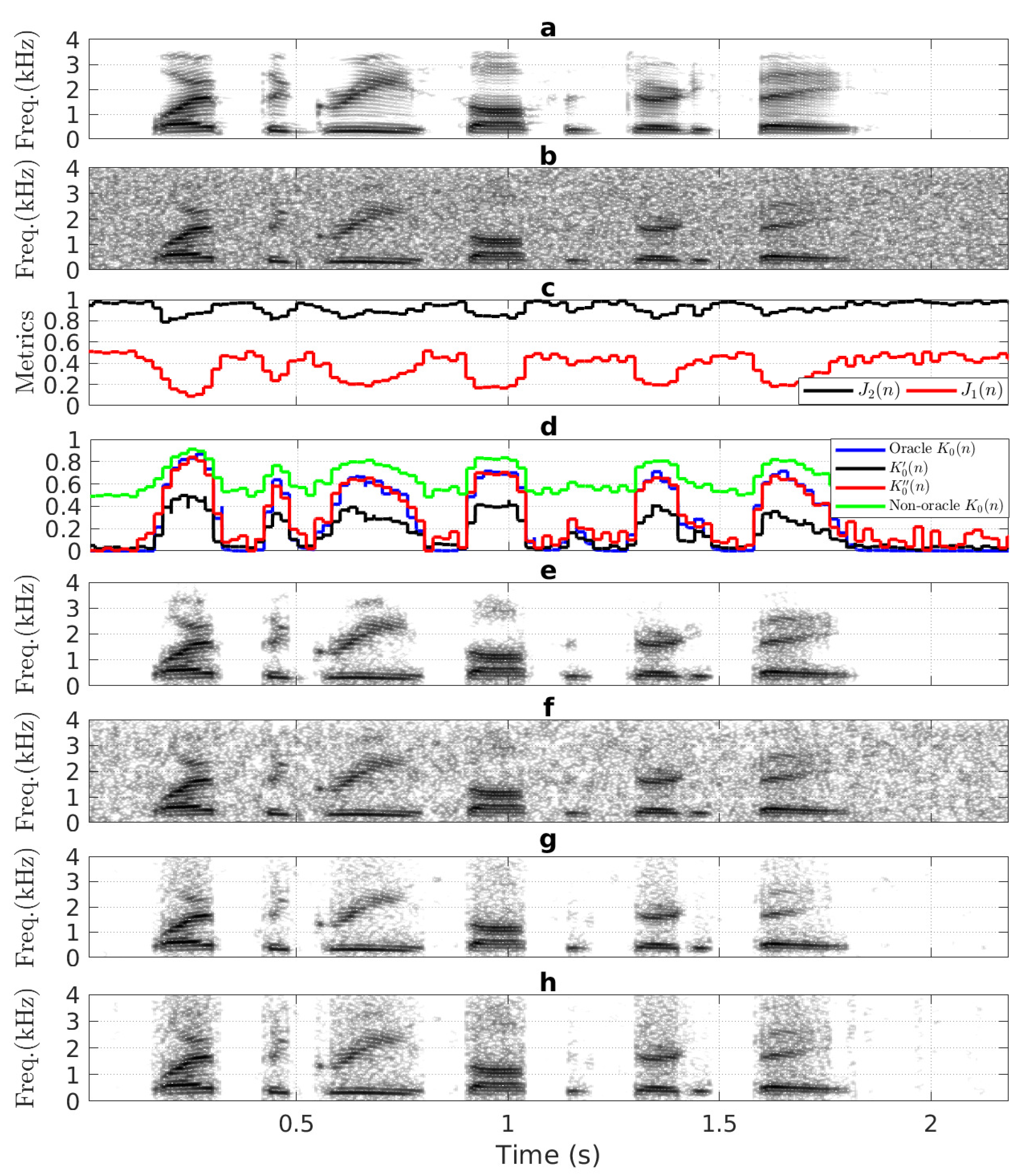
In [20], So et al. first analyze $K_0\left(n\right)$ in the oracle case, where ($\left\{a_i\right\},{\sigma }_w^2$) ($p=10$) and ${\sigma }_v^2$ are computed from each frame of the clean speech and the noise signal, $s(n,k)$ and $v(n,k)$. It can be seen that $K_0\left(n\right)$ approaches 1 when there is speech presence of the noisy speech, which passes almost clean speech to the output (e.g., 0.16–0.33 s or 0.9–1.06 s in Figure 1d,e). Conversely, $K_0\left(n\right)$ remains at approximately 0 during speech absence of the noisy speech, which does not pass any corrupting noise (e.g., 0–0.15 s or 1.8–2.19 s in Figure 1d,e). As a result, the KF-oracle method produces enhanced speech with less residual background noise as well as less speech distortion (Figure 1e).

In the non-oracle case, ($\left\{a_i\right\},{\sigma }_w^2$) are computed from noisy speech, resulting in biased ($\left\{{\tilde{a}}_i\right\},{\tilde{\sigma }}_w^2$). Then, $K_0\left(n\right)$ in (21) using biased ${\tilde{\sigma }}_w^2$ is given by:

$${\tilde{K}}_0\left(n\right)=\frac{{\alpha }^2\left(n\right)+{\tilde{\sigma }}_w^2}{{\alpha }^2\left(n\right)+{\tilde{\sigma }}_w^2+{\sigma }_v^2}.$$

(30)

In [20,21], So et al. assumed that the impact of WGN in $\left\{{\tilde{a}}_i\right\}$ is negligible. Thus, ${\tilde{\sigma }}_w^2$ could be approximately estimated as: ${\tilde{\sigma }}_w^2\approx {\sigma }_w^2+{\sigma }_v^2$ [20,21]. Substituting ${\tilde{\sigma }}_w^2\approx {\sigma }_w^2+{\sigma }_v^2$ in Equation (29) and re-arranging yields:

$${\tilde{K}}_0\left(n\right)=\frac{{\alpha }^2\left(n\right)+{\sigma }_w^2+{\sigma }_v^2}{{\alpha }^2\left(n\right)+{\sigma }_w^2+2{\sigma }_v^2}.$$

(31)

During speech pauses of $y(n,k)$, $s(n,k)=0$ gives ${\alpha }^2\left(n\right)=0$ and ${\sigma }_w^2=0$. According to Equation (30), ${\tilde{K}}_0\left(n\right)$ becomes biased around 0.5 (e.g., 0–0.15 s or 1.8–2.19 s in Figure 1d). As a result, ${\tilde{K}}_0\left(n\right)$ leak a significant amount of residual noise in the enhanced speech, as shown in Figure 1f.

In the non-oracle case, it is also observed that $J_2\left(n\right)\approx 1$ typically during speech pauses of $y(n,k)$ (e.g., 0–0.15 s or 1.8–2.19 s in Figure 1c). Therefore, the $J_2\left(n\right)$ metric is found to be useful in tuning biased $K_0\left(n\right)$ as [20]:

$$\begin{array}{c}\hfill K_0^{\prime }\left(n\right)={\tilde{K}}_0\left(n\right)[1-J_2\left(n\right)].\end{array}$$

(32)

Figure 1d reveals that $K_0^{\prime }\left(n\right)\approx 0$ during speech pauses. However, $K_0^{\prime }\left(n\right)$ is over-suppressed during speech presence of $y(n,k)$, resulting in distorted speech, as shown in Figure 1g.

To address this, So et al. proposed a $J_1\left(n\right)$ metric-based tuning of ${\tilde{K}}_0\left(n\right)$ [21]. It can be seen from Figure 1c that $J_1\left(n\right)$ lies around 0.5 during speech pauses (e.g., 0–0.15 s or 1.8–2.19 s), whereas it approaches 0 at speech regions (e.g., 0.16–0.33 s or 0.9–1.06 s). Therefore, the tuning of ${\tilde{K}}_0\left(n\right)$ using the $J_1\left(n\right)$ metric is performed as [21]:

$$\begin{array}{c}\hfill K_0^{″}\left(n\right)={\tilde{K}}_0\left(n\right)-J_1\left(n\right).\end{array}$$

(33)

It can be seen from Figure 1d that $K_0^{″}\left(n\right)$ is closely similar to the oracle $K_0\left(n\right)$, which minimizes distortion in the enhanced speech (Figure 1h) as compared to Figure 1g.

Technically, the real-life noise (colored/non-stationary) may contain time varying amplitudes, which impact ($\left\{a_i\right\},{\sigma }_w^2$) significantly as opposed to negligible impact of WGN in these parameters [20,21]. Therefore, the assumption of ${\tilde{\sigma }}_w^2\ne {\sigma }_w^2+{\sigma }_v^2$ made in [20,21] is invalid for real-life noise conditions. Moreover, the existing methods [20,21] do not analyze the impact of noise variance, ${\sigma }_v^2$ on $K_0\left(n\right)$. According to Equation (21), in addition to ${\alpha }^2\left(n\right)$ and ${\sigma }_w^2$, ${\sigma }_v^2$ is also an important parameter to compute $K_0\left(n\right)$ accurately. In light of these observations, the methods in [20,21] are not applicable for speech enhancement in real-life noise conditions. Therefore, we performed a detailed analysis of the biasing effect of $K_0\left(n\right)$ on KF-based speech enhancement in real-life noise conditions.

2.3. Impact of Biased $K_0\left(n\right)$ on KF-Based Speech Enhancement in Real-Life Noise Conditions

To analyze $K_0\left(n\right)$ and its impact on KF-based speech enhancement, we repeated the experiment in Figure 1, except that the utterance sp05 was corrupted with a typical real-life non-stationary noise, babble [24], at 5 dB SNR. A 32 ms rectangular window with 50% overlap ([25], Section 7.2.1) was considered for converting $y\left(n\right)$ into frames, $y(n,k)$ (as in Equation (28)).

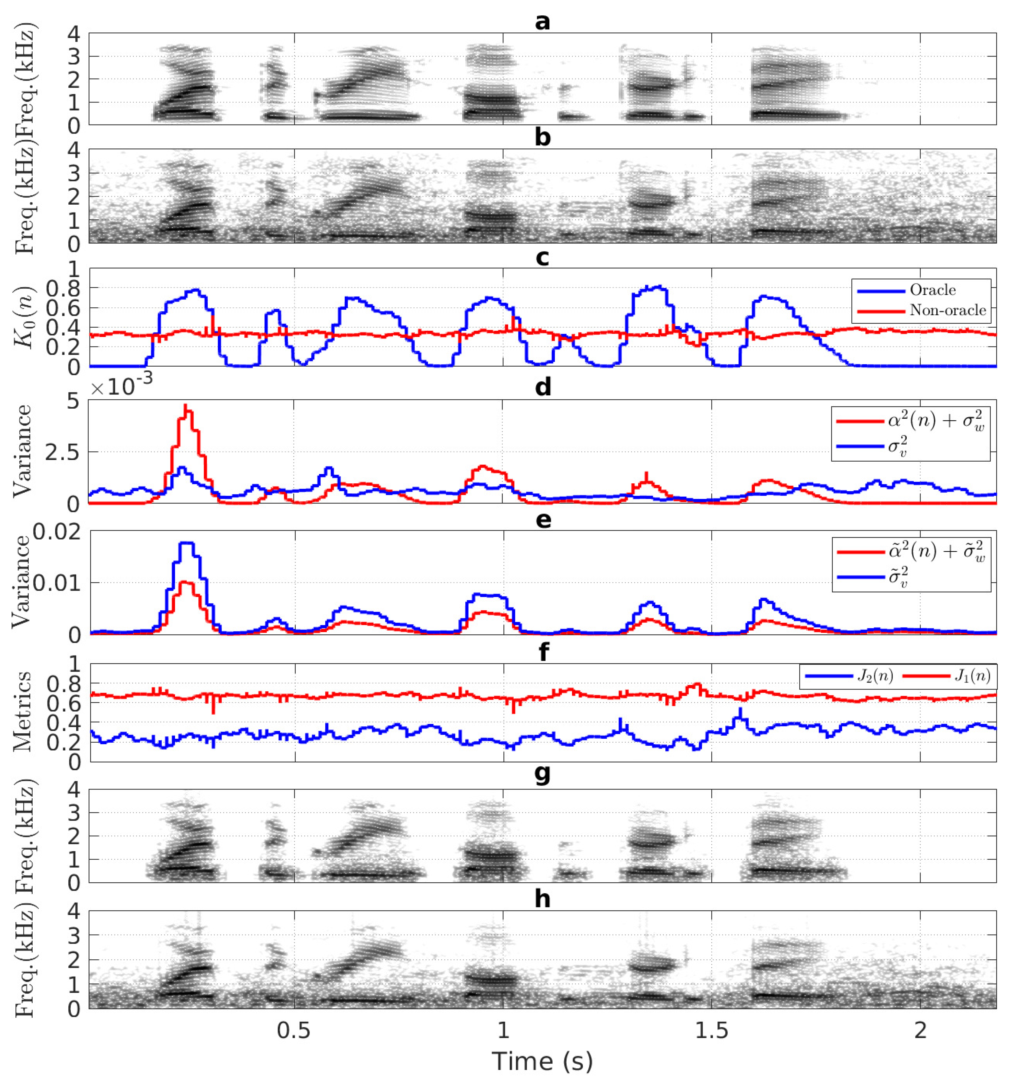
As shown in Section 2.2, in the oracle case, $K_0\left(n\right)$ also shows a smooth transition between 0 and 1 depending on the speech absence and speech presence of noisy speech (Figure 2c). Technically, during speech pauses of $y(n,k)$, the total a priori prediction error of the AR model, $[{\alpha }^2\left(n\right)+{\sigma }_w^2]=0$ (e.g., 0–0.15 s or 1.8–2.19 s in Figure 2d). Substituting $[{\alpha }^2\left(n\right)+{\sigma }_w^2]=0$ in Equation (21)) gives $K_0\left(n\right)=0$, which in turn yields $\widehat{s}\left(n\right|n)=0$ (Equation (23)), i.e., nothing is passed to the output (e.g., 0–0.15 s or 1.8–2.19 s of Figure 2c,g). Conversely, it was observed that $[{\alpha }^2\left(n\right)+{\sigma }_w^2]>>{\sigma }_v^2$ in speech regions of $y(n,k)$, for which $K_0\left(n\right)$ is approaching 1 (e.g., 0.16–0.33 s or 0.9–1.06 s in Figure 2c). As demonstrated in Section 2.2, a higher $K_0\left(n\right)$ enables the KF to produce enhanced speech with less residual background noise as well as less distortion (Figure 2g).

In the non-oracle case, the biased estimates of ($\left\{{\tilde{a}}_i\right\},{\tilde{\sigma }}_w^2$) and ${\tilde{\sigma }}_v^2$, resulted in $[{\tilde{\alpha }}^2\left(n\right)+{\tilde{\sigma }}_w^2]\approx {\tilde{\sigma }}_v^2$ (e.g., 0–0.15 s or 1.8–2.19 s in Figure 2e). According to Equation (21), this condition introduces around 0.5 bias in ${\tilde{K}}_0\left(n\right)$ (e.g., 0–0.15 s or 1.8–2.19 s in Figure 2c). During speech presence of $y(n,k)$, it is observed that ${\tilde{\sigma }}_v^2>>[{\tilde{\alpha }}^2\left(n\right)+{\tilde{\sigma }}_w^2]$ (e.g., 0.16–0.33 s or 0.9–1.06 s of Figure 2e), resulting in an underestimated ${\tilde{K}}_0\left(n\right)$ as compared to the oracle case (Figure 2c). The 0.5 biased ${\tilde{K}}_0\left(n\right)$ leaks 50% residual noise to $\widehat{s}\left(n\right|n)$ particularly in silent regions (Figure 2h). Additionally, the underestimated ${\tilde{K}}_0\left(n\right)$ in the speech regions introduce a significant distortion in the enhanced (Figure 2h). In addition, $J_2\left(n\right)$ and $J_1\left(n\right)$ metrics (Figure 2f) do not comply with the desired characteristics as found in WGN condition (Figure 1c). Therefore, it is inappropriate to apply $J_2\left(n\right)$ and $J_1\left(n\right)$ metrics in Figure 2f for tuning of the biased ${\tilde{K}}_0\left(n\right)$ (Figure 2c) using Equations (31) and (32).

In the AKF-RMBT method, the speech LPC parameters were computed from the pre-whitened speech to utilize $J_2\left(n\right)$ metric for the tuning of biased $K_0\left(n\right)$ in colored noise conditions ([22], Figure 5d). As in [20], $J_2\left(n\right)$ metric-based tuning of $K_0\left(n\right)$ still produces distorted speech. In addition, the noise LPC parameters computed from initial speech pauses keep constant during the processing of all noisy speech frames for an utterance. The whitening filter was also constructed with the constant noise LPCs to pre-whiten each noisy speech frame prior to compute speech LPC parameters. As a result, the tuning of $K_0\left(n\right)$ [22] becomes irrelevant in conditions having time-varying amplitudes, such as babble noise.

Motivated by the shortcomings of [20,21,22], we propose a $J_2\left(n\right)$ and $J_1\left(n\right)$ metric-based tuning of the KF gain, $K_0\left(n\right)$, for speech enhancement in real-life noise conditions.

3. Proposed Speech Enhancement Algorithm

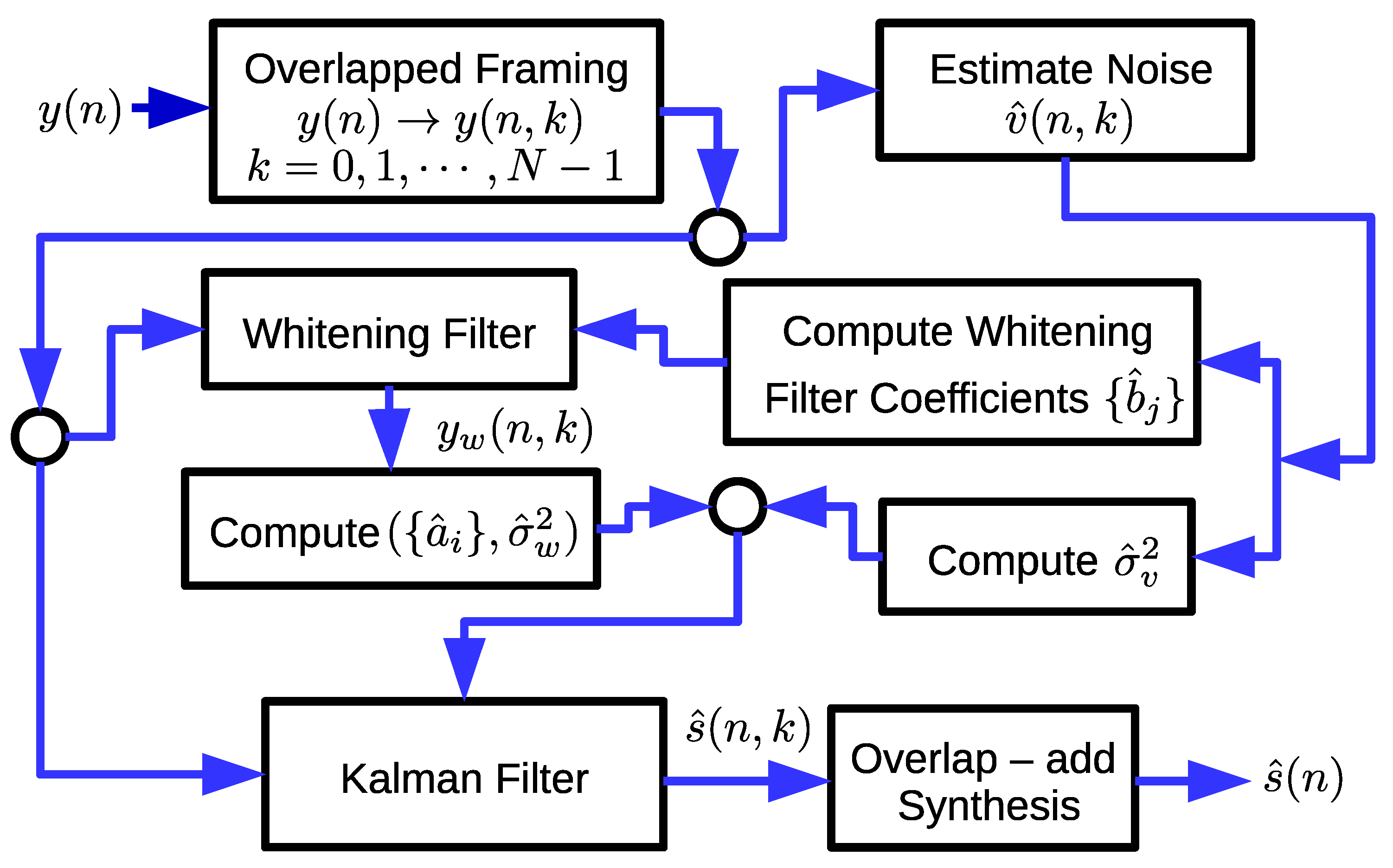
Figure 3 shows the block diagram of the proposed SEA. Firstly, $y\left(n\right)$ is converted into frames $y(n,k)$ with the same setup as used in Section 2.3.

To carry out the tuning of $K_0\left(n\right)$ in real-life noise conditions, unlike biased $J_2\left(n\right)$ and $J_1\left(n\right)$ metrics (Figure 2f), they should achieve similar characteristics that occur in the WGN condition (Figure 1c). It can be achieved through improving the estimates of ($\left\{{\widehat{a}}_i\right\},{\widehat{\sigma }}_w^2$) and ${\widehat{\sigma }}_v^2$ as described in Section 3.1.

3.1. Parameter Estimation

In is known that ($\left\{a_i\right\},{\sigma }_w^2$) are very sensitive to real-life noises. Since clean speech, $s(n,k)$, is unavailable in practice, it is difficult to accurately estimate these parameters. Therefore, we first focused on noise estimation, $\widehat{v}(n,k)$, for each noisy speech frame using speech presence probability (SPP) method (described in Section 3.2) [26] to compute ${\widehat{\sigma }}_v^2$. Given $\widehat{v}(n,k)$, ${\widehat{\sigma }}_v^2$ is computed as:

$$\begin{array}{c}\hfill {\widehat{\sigma }}_v^2=\frac{1}{M}\sum _{n=0}^{M-1}{\widehat{v}}^2(n,k).\end{array}$$

(34)

To reduce bias in the estimated ($\left\{{\widehat{a}}_i\right\},{\widehat{\sigma }}_w^2$) for each noisy speech frame, we computed them from the corresponding pre-whitened speech, $y_w(n,k)$ using the autocorrelation method [23]. The framewise $y_w(n,k)$ was obtained by applying a whitening filter, $H_w\left(z\right)$ to $y(n,k)$. $H_w\left(z\right)$ is given by [23]:

$$\begin{array}{c}\hfill H_w\left(z\right)=1+\sum _{j=1}^q{\widehat{b}}_j{z}^{-j},\end{array}$$

(35)

where the coefficients, $\left\{{\widehat{b}}_j\right\}$ ($q=20$) are computed from $\widehat{v}(n,k)$ using the autocorrelation method [23].

3.2. Proposed $\widehat{v}(n,k)$ Estimation Method

The proposed noise estimation is performed in the acoustic domain using the SPP method [26]. For more details about the SPP method, we refer the readers to [26]. However, we briefly review the SPP-based noise estimation in this section. For this purpose, the noisy speech, $y\left(n\right)$ (Equation (1)) is analyzed frame-wise using the short-time Fourier transform (STFT):

$$Y_k\left(m\right)=S_k\left(m\right)+V_k\left(m\right),$$

(36)

where $Y_k\left(m\right)$, $S_k\left(m\right)$, and $V_k\left(m\right)$ denote the complex-valued STFT coefficients of the noisy speech, the clean speech, and the noise signal, respectively, for time-frame index k and frequency bin index $mϵ\{0,1,\dots ,255\}$.

A Hamming window with 50% overlap was used in STFT analysis ([25], Section 7.2.1). In polar form, $Y_k\left(m\right)$, $S_k\left(m\right)$, and $V_k\left(m\right)$ can be expressed as: $Y_k\left(m\right)=R_k\left(m\right)e^{j{\varphi }_k\left(m\right)}$, $S_k\left(m\right)=A_k\left(m\right)e^{j{\phi }_k\left(m\right)}$, and $V_k\left(m\right)=D_k\left(m\right)e^{j{\theta }_k\left(m\right)}$, where $R_k\left(m\right)$, $A_k\left(m\right)$, and $D_k\left(m\right)$ are the magnitude spectra of the noisy speech, the clean speech, and the noise signal, respectively, and ${\varphi }_k\left(m\right)$, ${\phi }_k\left(m\right)$, and ${\theta }_k\left(m\right)$ are the corresponding phase spectra. We processed each frequency bin of the single-sided noisy speech power spectrum, $R_k^2\left(m\right)$, to estimate the noise power spectrum, ${\widehat{D}}_k^2\left(m\right)$, where $mϵ\{0,1,\dots ,128\}$ contain the DC and Nyquist frequency components. To initialize the algorithm, we considered the first frame ($k=0$) of $R_0^2\left(m\right)$ as silent, giving an estimate of noise power, ${\widehat{D}}_0^2\left(m\right)=R_0^2\left(m\right)$. The noise PSD, ${\widehat{\lambda }}_0\left(m\right)$, was also initialized as ${\widehat{\lambda }}_0\left(m\right)={\widehat{D}}_0^2\left(m\right)$. For $k\ge 1$; using the speech presence uncertainty principle [26], an MMSE estimate of ${\widehat{D}}_k^2\left(m\right)$ at $m^{th}$ frequency bin is given by:

$$\begin{array}{cc}\hfill {\widehat{D}}_k^2\left(m\right)& =P\left(H_0^m\right|R_k\left(m\right))R_k^2\left(m\right)+P\left(H_1^m\right|R_k\left(m\right)){\widehat{\lambda }}_{k-1}\left(m\right),\hfill \end{array}$$

(37)

where $P\left(H_0^m\right|R_k\left(m\right))$ and $P\left(H_1^m\right|R_k\left(m\right))$ are the conditional probability of the speech absence and the speech presence given $R_k\left(m\right)$ at $m^{th}$ frequency bin.

The simplified $P\left(H_1^m\right|R_k\left(m\right))$ estimate is given by (The simplification is a result of assuming the a priori probability of the speech absence and presence, $P\left(H_0\right)$ and $P\left(H_1\right)$ as: $P\left(H_0\right)=P\left(H_1\right)$ [26].):

$$\begin{array}{c}\hfill P\left(H_1^m\right|R_k\left(m\right))={\left[1+(1+{\xi }_{opt})exp\left\{\left(-\frac{R_k^2\left(m\right)}{{\widehat{\lambda }}_{k-1}\left(m\right)}\right)\left(\frac{{\xi }_{opt}}{1+{\xi }_{opt}}\right)\right\}\right]}^{-1},\end{array}$$

(38)

where ${\xi }_{opt}$ is the optimal a priori SNR.

In [26], the optimal choice for ${\xi }_{opt}$ is found to be $10{log}_{10}\left({\xi }_{opt}\right)=15$ dB, and $P\left(H_0^m\right|R_k\left(m\right))$ is given by $P\left(H_0^m\right|R_k\left(m\right))=1-P\left(H_1^m\right|R_k\left(m\right))$. If $P\left(H_1^m\right|R_k\left(m\right))=1$ occurs at $m^{th}$ frequency bin, it causes stagnation, which stops updating ${\widehat{D}}_k^2\left(m\right)$ (Equation (37)). Unlike monitoring the status of $P\left(H_1^m\right|R_k\left(m\right))=1$ for a long time as reported in [26], we simply resolve this issue by setting $P\left(H_1^m\right|R_k\left(m\right))=0.99$ once this condition occurs prior to updating ${\widehat{D}}_k^2\left(m\right)$.

It was observed that $R_k^2\left(m\right)$ was completely filled with additive noise during silent activity, thus giving an estimate of noise power. Therefore, unlike updating ${\widehat{D}}_k^2\left(m\right)$ using Equation (36) by an existing method [26], we achieved this differently depending on the silent/speech activity of $R_k^2\left(m\right)$ (for each frequency bin m). Specifically, at $m^{th}$ frequency bin ($k\ge 1$), if $P\left(H_1^m\right|R_k\left(m\right))<0.5$, $R_k^2\left(m\right)$ yields silent activity, resulting in ${\widehat{D}}_k^2\left(m\right)=R_k^2\left(m\right)$; otherwise, ${\widehat{D}}_k^2\left(m\right)$ is estimated using Equation (37). With estimated ${\widehat{D}}_k^2\left(m\right)$, ${\widehat{\lambda }}_k\left(m\right)$ is updated as:

$${\widehat{\lambda }}_k\left(m\right)=\eta {\widehat{\lambda }}_{k-1}\left(m\right)+(1-\eta ){\widehat{D}}_k^2\left(m\right),$$

(39)

where the smoothing constant, $\eta$ is set to 0.9.

The |IDFT| of $P_v\left(m\right)e^{j{\varphi }_k\left(m\right)}$ yields the estimated noise, $\widehat{v}(n,k)$, where $P_v\left(m\right)=\sqrt{{\widehat{\lambda }}_k\left(m\right)}$. To ensure the conjugate symmetry, the components of $P_v\left(m\right)$ at $mϵ\{1,2,\dots ,127\}$ are flipped to that of the $mϵ\{129,130,\dots ,255\}$ of $P_v\left(m\right)$ before taking the |IDFT|. We can justify the improvement of $\widehat{v}(n,k)$ estimation using the SPP method [26] in terms of analyzing the tuning parameters of KF in Section 3.3.

3.3. Proposed $K_0\left(n\right)$ Tuning Method

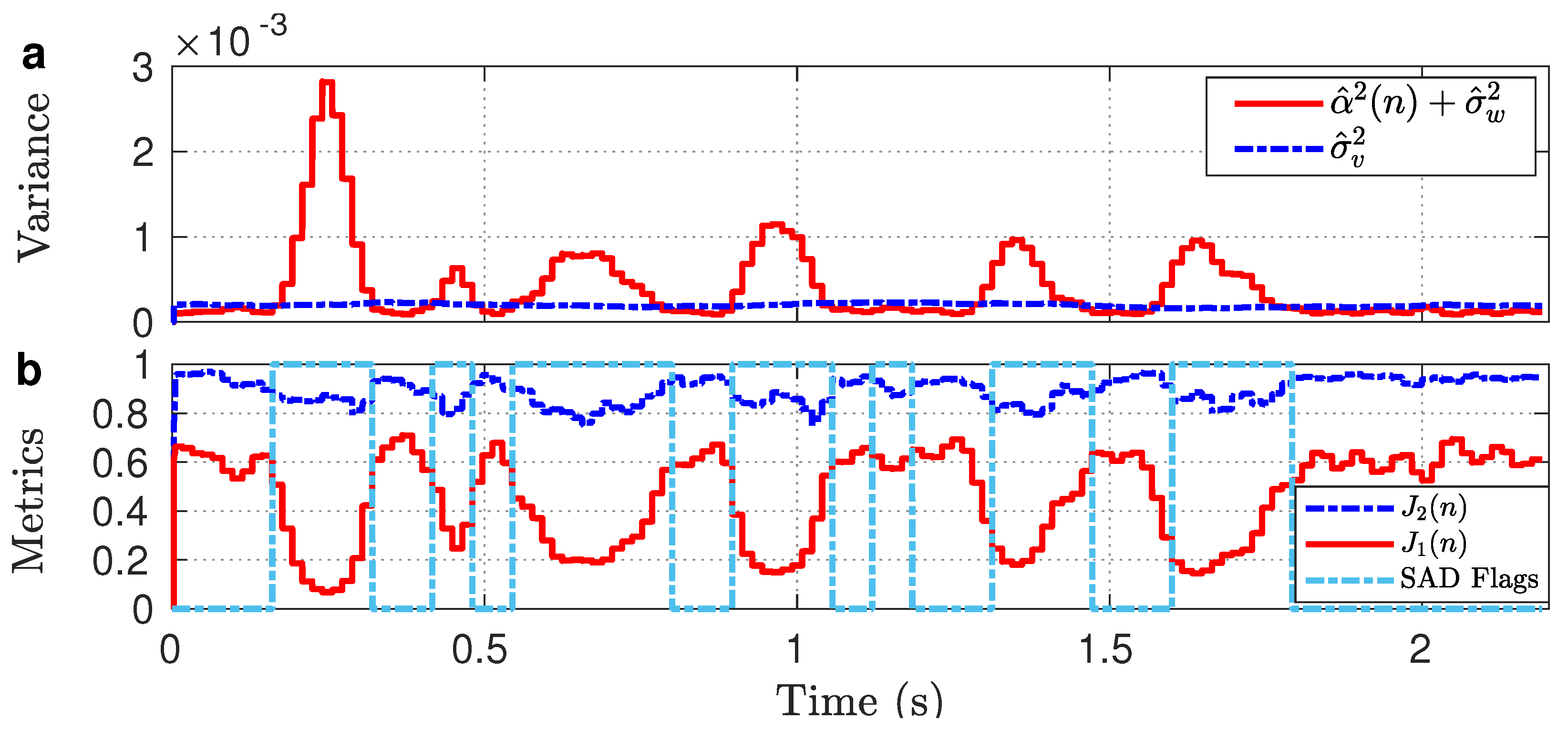
Firstly, we constructed KF with $(\left\{{\widehat{a}}_i\right\},{\widehat{\sigma }}_w^2)$ and ${\widehat{\sigma }}_v^2$ and extracted the tuning parameters as shown in Figure 4. It can be seen from Figure 4a that $[{\widehat{\alpha }}^2\left(n\right)+{\widehat{\sigma }}_w^2]$ achieves similar characteristics as the KF-oracle method (Figure 2d). Unlike ${\tilde{\sigma }}_v^2$ in the non-oracle case (Figure 2e), ${\widehat{\sigma }}_v^2$ becomes lower than $[{\widehat{\alpha }}^2\left(n\right)+{\widehat{\sigma }}_w^2]$, as usually occurred in the oracle case (Figure 2d). The improvement of these parameters also enables $J_2\left(n\right)$ and $J_1\left(n\right)$ metrics (Figure 4b) to achieve quite similar characteristics as appear in the WGN condition (Figure 1c). Therefore, $J_2\left(n\right)$ and $J_1\left(n\right)$ metrics (Figure 4b) are now eligible to dynamically tune $K_0\left(n\right)$ in real-life noise conditions. However, our investigation reveals that the $J_2\left(n\right)$ metric is useful in tuning $K_0\left(n\right)$ during speech pauses, since it is underestimated $K_0\left(n\right)$ during speech presence of noisy speech [21]. On the contrary, since the $J_1\left(n\right)$ metric approaches 0 in speech regions of noisy speech, according to eq. (32), it minimizes the underestimation of $K_0\left(n\right)$. In light of these observations, for each sample of $y(n,k)$, we incorporated the $J_2\left(n\right)$ metric during speech pauses and the $J_1\left(n\right)$ metric during speech presence to dynamically offset the bias in ${\tilde{K}}_0\left(n\right)$.

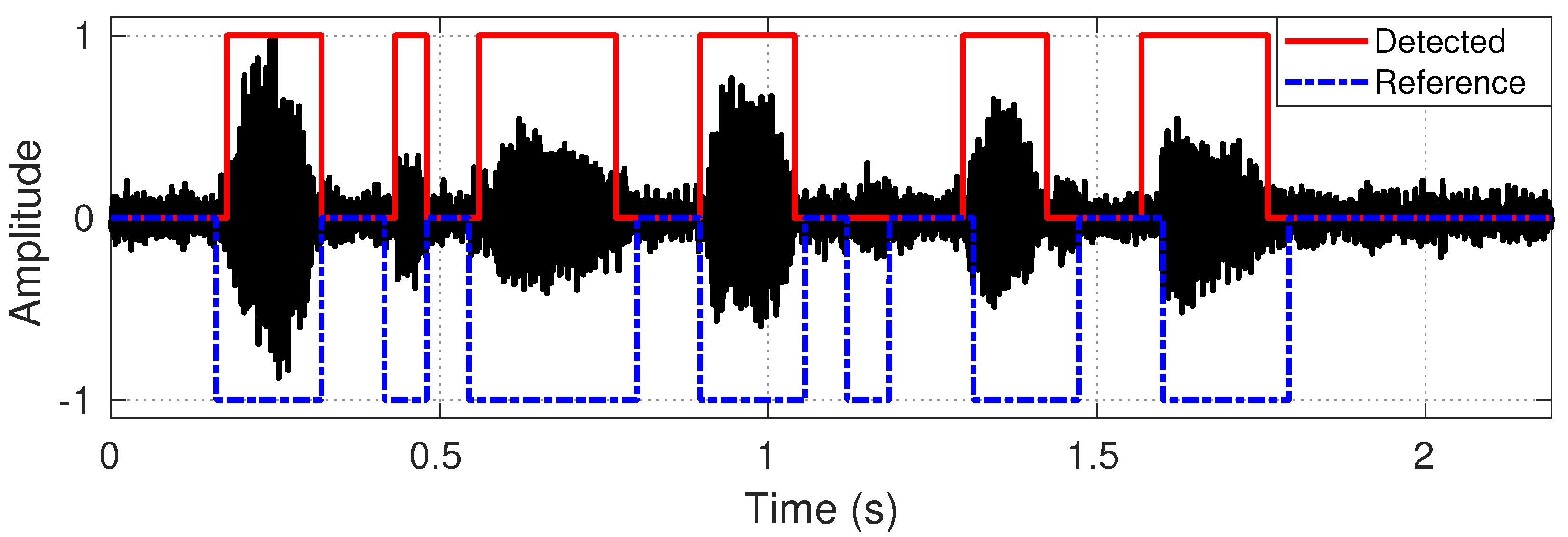
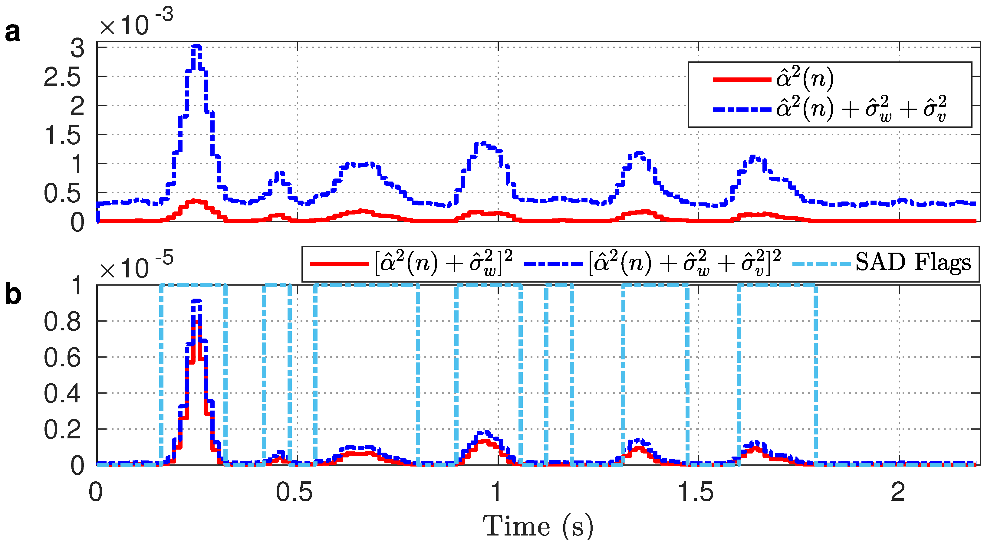
The proposed tuning algorithm requires a speech activity detector that operates on a sample-by-sample basis. However, the existing speech activity detector operates on a frame-by-frame basis. In addition, the incorporation of any external speech activity detector makes the proposed tuning algorithm a bit complex. To cope with the issues, we studied and found that the KF parameters can be adopted as a speech activity detector that operates on a sample-by-sample basis. Specifically, we found that $[{\widehat{\alpha }}^2\left(n\right)+{\widehat{\sigma }}_w^2]$ and ${\widehat{\sigma }}_v^2$ can be adopted as a speech activity detector for each sample of $y(n,k)$. For example, during speech pauses, the condition ${\widehat{\sigma }}_v^2\ge [{\widehat{\alpha }}^2\left(n\right)+{\widehat{\sigma }}_w^2]$ holds (e.g., 0–0.15 s or 1.8–2.19 s of Figure 4a. Conversely, $[{\widehat{\alpha }}^2\left(n\right)+{\widehat{\sigma }}_w^2]>>{\widehat{\sigma }}_v^2$ is found in speech regions (e.g., 0.16–0.33 s or 0.9–1.06 s of Figure 4a). Therefore, at sample n, if ${\widehat{\sigma }}_v^2\ge [{\widehat{\alpha }}^2\left(n\right)+{\widehat{\sigma }}_w^2]$, $y(n,k)$ is termed as silent and set the decision parameter (denoted by $\zeta$) as $\zeta \left(n\right)=0$; otherwise, speech activity occurs and $\zeta \left(n\right)=1$. Figure 5 reveals that the detected flags (0/1: silent/speech) by the proposed method are closely similar to that of the reference (0/−1: silent/speech, generated by visually inspecting the utterance sp05).

At sample n, if $\zeta \left(n\right)=0$, the adjusted $K_0^{\prime }\left(n\right)$ in the proposed SEA is given by:

$$\begin{array}{cc}\hfill & K_0^{\prime }\left(n\right)={\tilde{K}}_0\left(n\right)[1-J_2\left(n\right)],\hfill \\ \hfill & =\left[\frac{{\widehat{\alpha }}^2\left(n\right)+{\widehat{\sigma }}_w^2}{{\widehat{\alpha }}^2\left(n\right)+{\widehat{\sigma }}_w^2+{\widehat{\sigma }}_v^2}\right] \left[\frac{{\widehat{\alpha }}^2\left(n\right)}{{\widehat{\alpha }}^2\left(n\right)+{\widehat{\sigma }}_w^2}\right],\hfill \\ \hfill & =\frac{{\widehat{\alpha }}^2\left(n\right)}{{\widehat{\alpha }}^2\left(n\right)+{\widehat{\sigma }}_w^2+{\widehat{\sigma }}_v^2}.\hfill \end{array}$$

(40)

To justify the validity of $K_0^{\prime }\left(n\right)$, Figure 6a shows the numerator and the denominator of Equation (40) computed from the noisy speech in Figure 2b. It can be seen that ${\widehat{\alpha }}^2\left(n\right)\approx 0$ during speech pauses (e.g., 0–0.15 s or 1.8–2.19 s of Figure 6a). According to Equation (40), $K_0^{\prime }\left(n\right)\approx 0$. Since $[{\widehat{\alpha }}^2\left(n\right)+{\widehat{\sigma }}_w^2+{\widehat{\sigma }}_v^2]>>{\widehat{\alpha }}^2\left(n\right)$ occurs during speech presence (e.g., 0.16–0.33 s or 0.9–1.06 s of Figure 6a), it may be underestimated $K_0^{\prime }\left(n\right)$ as in the WGN experiment (Figure 1d). Thus, $J_2\left(n\right)$ metric-based tuning of $K_0^{\prime }\left(n\right)$ in speech activity of $y(n,k)$ is inappropriate.

As discussed earlier, we carried out tuning biased $K_0\left(n\right)$ using the $J_1\left(n\right)$ metric during speech activity of $y(n,k)$. However, our further investigation of the $J_1\left(n\right)$ metric-based tuning in Equation (33) reveals that the subtraction of $J_1\left(n\right)$ from biased $K_0\left(n\right)$ may still produce an underestimated $K_0^{\prime }\left(n\right)$. To cope with this problem, at sample n, if $\zeta \left(n\right)=1$, we found a more effective solution for tuning of biased $K_0\left(n\right)$ using the $J_1\left(n\right)$ metric as:

$$\begin{array}{cc}\hfill K_0^{\prime }\left(n\right)& ={\tilde{K}}_0\left(n\right)[1-J_1\left(n\right)],\hfill \\ \hfill & =\left[\frac{{\widehat{\alpha }}^2\left(n\right)+{\widehat{\sigma }}_w^2}{{\widehat{\alpha }}^2\left(n\right)+{\widehat{\sigma }}_w^2+{\widehat{\sigma }}_v^2}\right] \left[\frac{{\widehat{\alpha }}^2\left(n\right)+{\widehat{\sigma }}_w^2}{{\widehat{\alpha }}^2\left(n\right)+{\widehat{\sigma }}_w^2+{\widehat{\sigma }}_v^2}\right],\hfill \\ \hfill & =\frac{{[{\widehat{\alpha }}^2\left(n\right)+{\widehat{\sigma }}_w^2]}^2}{{[{\widehat{\alpha }}^2\left(n\right)+{\widehat{\sigma }}_w^2+{\widehat{\sigma }}_v^2]}^2}.\hfill \end{array}$$

(41)

To justify the validity of $K_0^{\prime }\left(n\right)$, the numerator and the denominator of Equation (41) are shown in Figure 6b. It can be seen that ${[{\widehat{\alpha }}^2\left(n\right)+{\widehat{\sigma }}_w^2+{\widehat{\sigma }}_v^2]}^2\ge {[{\widehat{\alpha }}^2\left(n\right)+{\widehat{\sigma }}_w^2]}^2$ during speech presence of $y(n,k)$ (e.g., 0.16–0.33 s or 0.9–1.06 s), which causes $K_0^{\prime }\left(n\right)$ to approach 1.

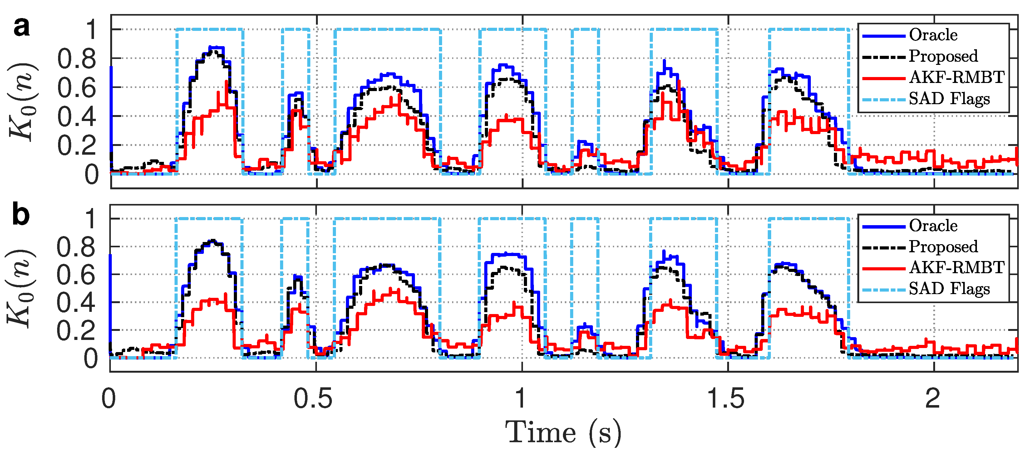
To examine the performance of the proposed tuning algorithm in real-life non-stationary noise conditions, we repeated the experiment in Figure 2. It can be seen from Figure 7a that $K_0^{\prime }\left(n\right)$ is closely similar to the oracle $K_0\left(n\right)$. Specifically, it maintains a smooth transition at the edges and the temporal changes in speech regions are closely matched to the oracle $K_0\left(n\right)$. Conversely, the AKF-RMBT method [22] produces a significant underestimated $K_0\left(n\right)$ in speech regions. Therefore, the reduced-biased $K_0^{\prime }\left(n\right)$ in the proposed method is more appropriate to mitigate the risks of distortion in the enhanced speech than that of the AKF-RMBT method [22]. We also repeated the experiment in Figure 2 except for the utterance sp05 which was corrupted by 5 dB colored (f16) noise. Figure 7b reveals that the biasing effect is reduced significantly in $K_0^{\prime }\left(n\right)$ and closely similar to the oracle $K_0\left(n\right)$. However, the AKF-RMBT method [22] still produced underestimated $K_0\left(n\right)$ in speech regions. In light of the comparative study, it is evident that the proposed method adequately addresses the tuning of biased $K_0\left(n\right)$ both in real-life non-stationary and colored noise conditions.

4. Speech Enhancement Experiment

4.1. Corpus

For the objective experiments, 30 phonetically balanced utterances belonging to six speakers (three male and three female) were taken from the NOIZEUS corpus ([1], Chapter 12). The clean speech recordings had lengths of two sec to four sec depending on utterances ([1], Chapter 12). We generated a noisy speech data set by mixing the clean speech with real-world non-stationary (babble, street) and colored (factory2 and f16) noise recordings at multiple SNR levels (from −5 dB to +15 dB, in 5 dB increments). This provided 30 examples per condition with 20 total conditions. The $street$ noise recording was taken from [27] and the rest of the noise recordings were taken from [24]. All clean speech and noise recordings in the noisy speech data set are single channel with a sampling frequency of 8 kHz.

4.2. Objective Evaluation

The objective measures were used to evaluate the quality and intelligibility of the enhanced speech with respect to the corresponding clean speech. The following objective evaluation metrics have been used in this paper:

• Perceptual Evaluation of Speech Quality (PESQ) for objective quality evaluation [28]. The PESQ score ranged between −0.5 and 4.5. A higher PESQ score indicates better speech quality;
• Signal to distortion ratio (SDR) for objective quality evaluation [29]. The SDR score ranged between $-\infty$ and $+\infty$. A higher SDR score indicates better speech quality;
• Short-time objective intelligibility (STOI) measure for objective intelligibility evaluation [30]. It ranged between 0 and 1 (or 0 and 100%). A higher STOI score indicates better speech intelligibility.

4.3. Spectrogram Evaluation

We also analyzed the spectrograms of enhanced speech produced by the proposed and the competitive methods to visually quantify the level of residual noise as well as distortion. For this purpose, we generated a noisy speech data set by corrupting the utterance sp05 with 5 dB babble (non-stationary) and 5 dB f16 (colored) noises.

4.4. Subjective Evaluation

The subjective evaluation was carried out through a series of blind AB listening tests ([5], Section 3.3.4). To perform these tests, we used the same noisy speech data set (Section 4.3). In this test, the enhanced speech produced by six SEAs as well as the corresponding clean speech and noise corrupted speech signals were played as stimuli pairs to the listeners. Specifically, the test was performed on a total of 112 stimuli pairs (56 for each utterance) played in a random order to each listener, excluding the comparisons for the same method.

The listener gave the following ratings for each stimuli pair: prefers the first or second stimuli, which is perceptually better, or a third response indicating no difference was found between them. For a pairwise scoring, 100% is given to the preferred method, 0% to the other, and 50% for the similar preference response. The participants could re-listen to stimuli if required. Ten English speaking listeners participated in the blind AB listening tests. The average of the preference scores given by the listeners is termed the mean preference score (%), which was used to compare the efficiency among the SEAs.

4.5. Specifications of the Competitive SEAs

The performance of the proposed SEA was carried out by comparing it with the following benchmark SEAs ($p:$ order of $\left\{a_i\right\}$, ${\sigma }_w^2$: the excitation variance of AR model, $w:$ analysis frame duration (ms), and $s:$ analysis frame shift (ms)).

• Noisy: No enhancement (speech corrupted with noise);
• KF-oracle: KF, where ($\left\{a_i\right\}$, ${\sigma }_w^2$) and ${\sigma }_v^2$ are computed from the clean speech and the noise signal, $p=10$, $w=32$ ms, $s=16$ ms, and a rectangular window is used for framing;
• KF-Non-oracle: KF, where ($\left\{a_i\right\}$, ${\sigma }_w^2$) and ${\sigma }_v^2$ are computed from the noisy speech, $p=10$, $w=32$ ms, $s=16$ ms, and rectangular window is used for framing;
• MMSE-STSA [9]: It used $w=25$ ms, $s=10$ ms, and Hamming window for framing;
• AKF-IT [13]: AKF operates with two iterations, where initial ($\left\{a_i\right\}$, ${\sigma }_w^2$) and ($\left\{b_j\right\}$, ${\sigma }_u^2$) are computed from the noisy speech followed by re-estimation of them from the processed speech after first iteration, $p=10$, noise LPC order $q=10$, $w=20$ ms, $s=0$ ms, and rectangular window is used for framing;
• AKF-RMBT [22]: Robustness metric-based tuning of the AKF, where ($\left\{a_i\right\}$, ${\sigma }_w^2$) and ($\left\{b_j\right\}$, ${\sigma }_u^2$) are computed from the pre-whitened speech and initial silent frames, $p=10$, $q=40$, $w=20$ ms, $s=0$ ms, and rectangular window is used for framing;
• MDKF-MMSE [17]: Modulation-domain KF, where ($\left\{a_i\right\}$, ${\sigma }_w^2$) is computed from the pre-filtered speech using the MMSE-STSA method [9], $p=2$, $q=4$, $w=20$ ms, $s=0$ ms in modulation domain;
• Proposed: Robustness and sensitivity tuning of the KF, where ($\left\{{\widehat{a}}_i\right\}$, ${\widehat{\sigma }}_w^2$) and ${\widehat{\sigma }}_v^2$ are computed from the pre-whitened speech and estimated noise, $p=20$, $q=20$, $w=32$ ms, $s=16$ ms, rectangular window is used for time-domain frames, and Hamming window is used for acoustic frames.

5. Results and Discussion

5.1. Objective Quality Evaluation

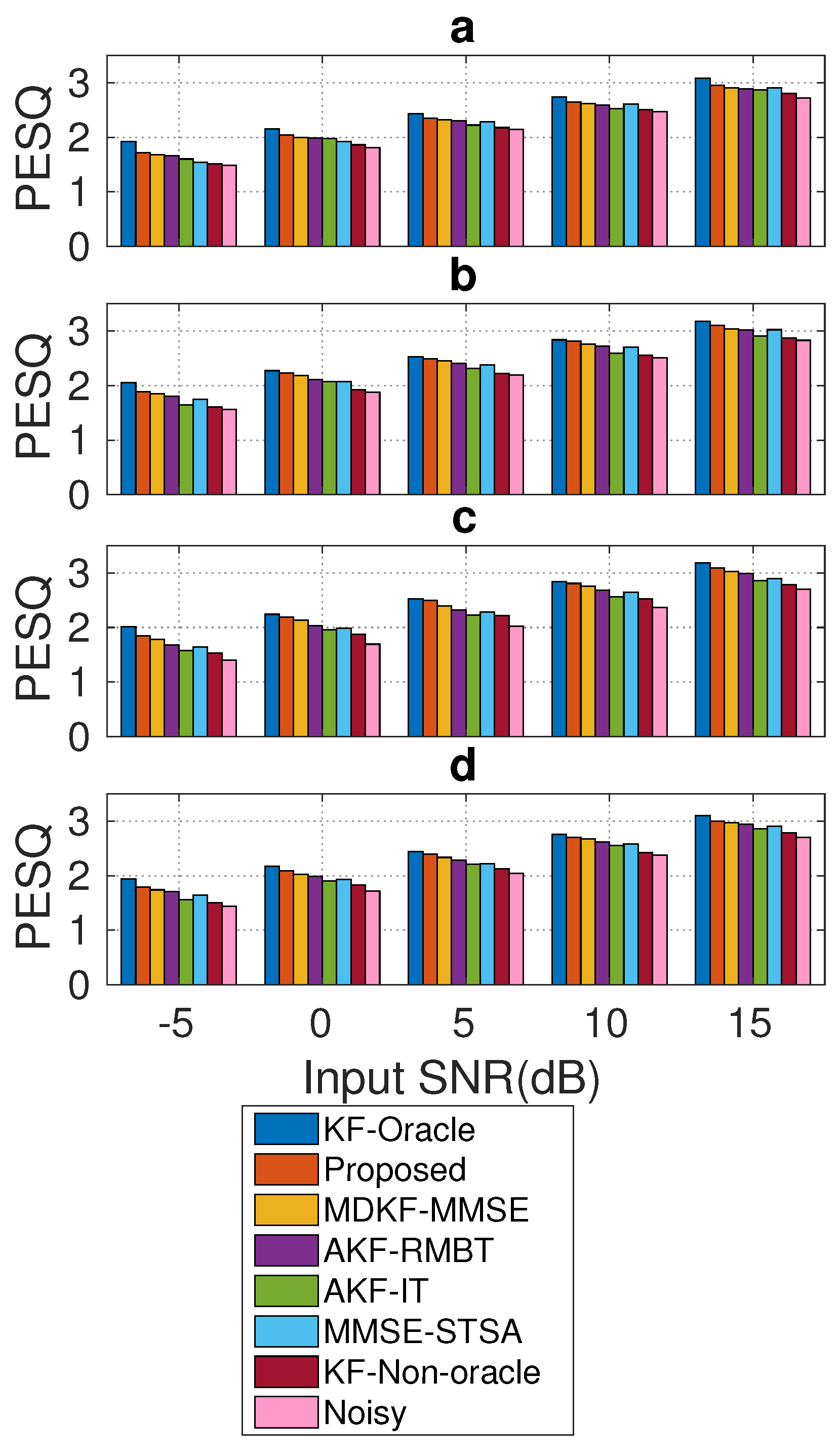
Figure 8 shows the average PESQ score (found over all frames for each test condition in Section 4.1) for each SEA. It can be seen that the KF-oracle method exhibits the highest PESQ score for all test conditions. It is due to ($\left\{a_i\right\}$, ${\sigma }_w^2$) and ${\sigma }_v^2$ being computed from the clean speech and the noise signal. The improvement of the average PESQ score for the KF-non-oracle method is marginal as compared to the noisy one. The proposed SEA shows a considerable PESQ score improvement compared to the benchmark methods across the test conditions. The average PESQ score for the proposed method is also very similar to that of the KF-oracle method. It is due to the reduced-biased Kalman gain obtained by the proposed tuning algorithm being closely similar to that of the KF-oracle method (Figure 7). Amongst the benchmark methods, MDKF-MMSE [17] shows relatively competitive PESQ scores followed by AKF-RMBT [22] for all tested conditions (Figure 9a–d). On the other hand, the AKF-IT method [13] exhibits reduced PESQ scores than other benchmark methods across the test conditions due to suffering from distortion and musical noise in the enhanced speech. In light of this comparative study, it is evident that the proposed method has better quality with regard to enhanced speech than that of the competing methods for all tested conditions.

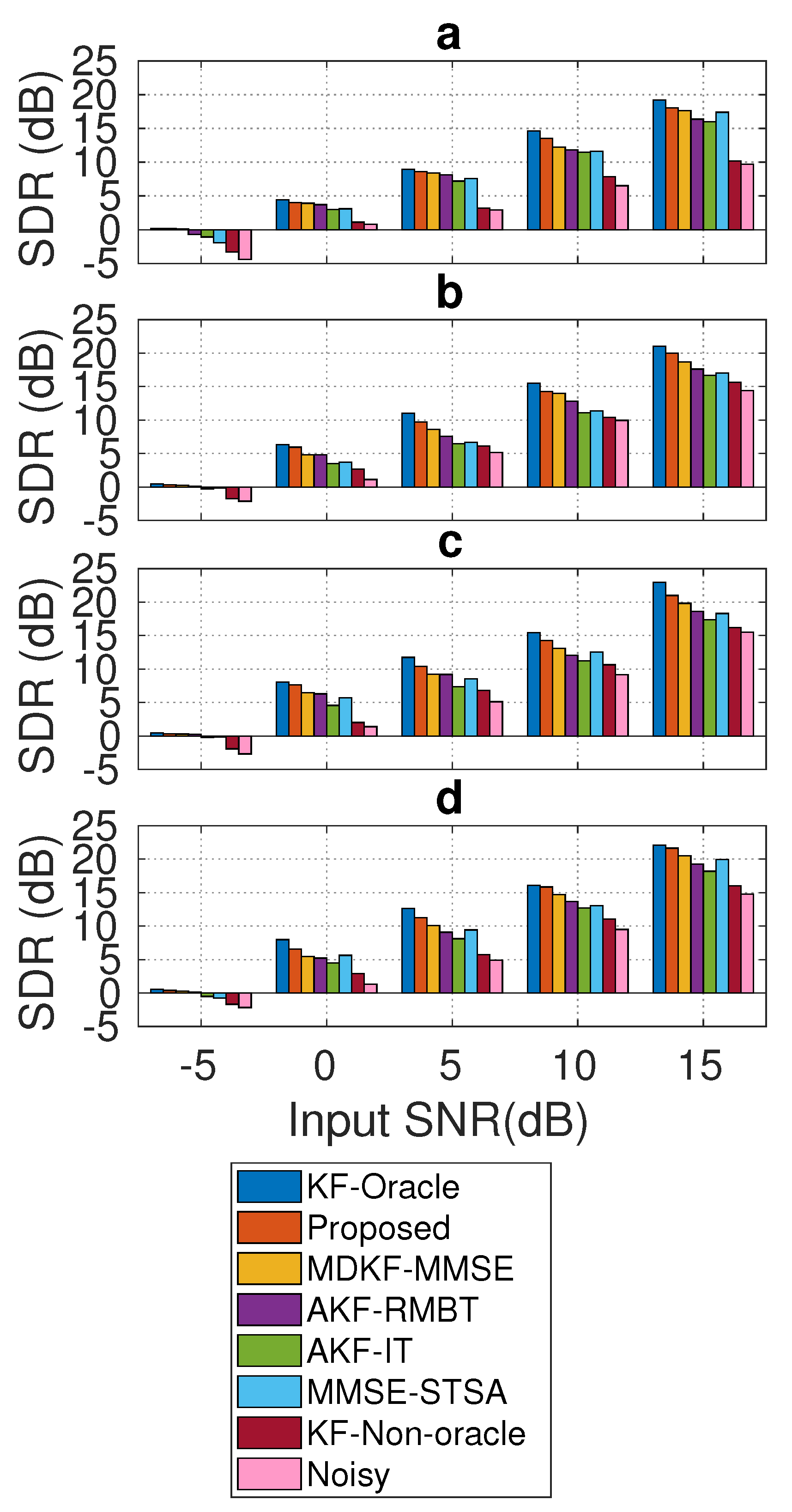
Figure 9 shows the average SDR (dB) score (found over all frames for each test condition in Section 4.1) for each SEA. Like the earlier experiment in Figure 8, the KF-oracle method shows an indication of the highest SDR score for all test conditions. Additionally, the noisy one shows the lower SDR scores for all tested conditions. The proposed SEA consistently demonstrates SDR score improvement from the competing methods across the test conditions. Amongst the competing methods, the MDKF-MMSE [17] show relatively competitive SDR scores for all tested conditions (Figure 9a–d). The noisy one shows the lowest SDR scores for all tested conditions. In light of this comparative study, it is evident that the proposed SEA exhibits less distortion in the enhanced speech than that of the competing methods for all tested conditions.

5.2. Objective Intelligibility Evaluation

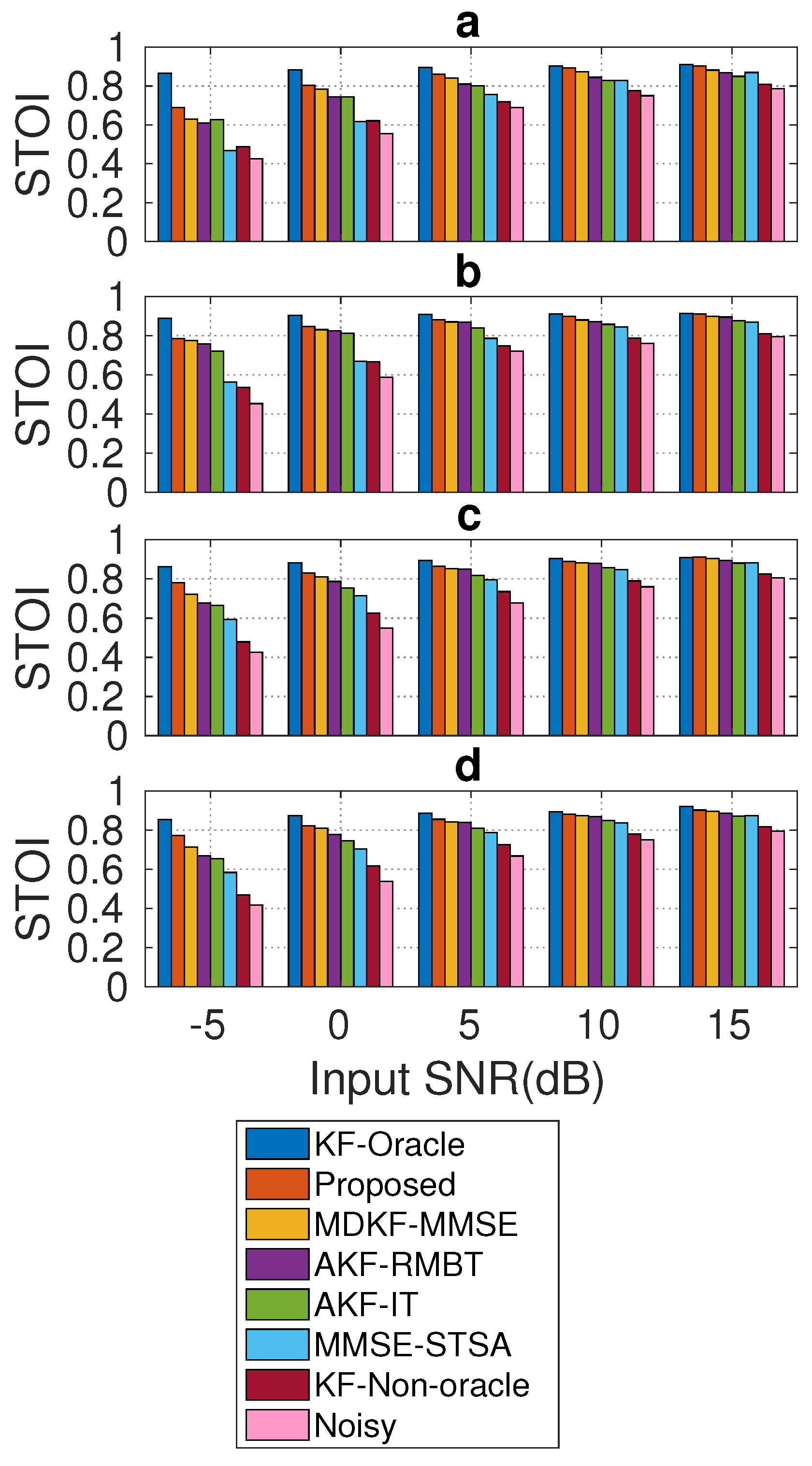
Figure 10 shows the average STOI score (found over all frames for each test condition in Section 4.1). Like the PESQ score comparison (Section 5.1), the KF-oracle method also achieves the highest STOI score for all tested conditions. The proposed method consistently outperforms all competing methods across the tested conditions in terms of STOI score improvements. The STOI score improvement by the proposed method is also very similar to that of the KF-oracle method. Amongst the benchmark methods, MDKF-MMSE [17] is found to be competitive with the proposed method for all tested conditions. Conversely, the noisy one shows the lowest STOI scores for all tested conditions. In light of this comparative study, it is evident that the proposed method produces better intelligible enhanced speech than the competing methods for all tested conditions.

5.3. Spectrogram Analysis of the SEAs

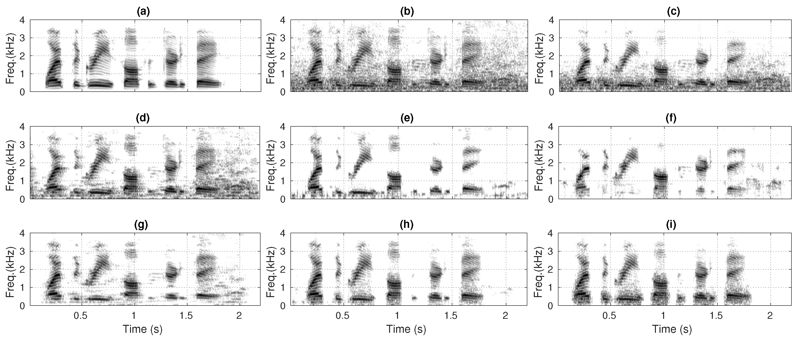
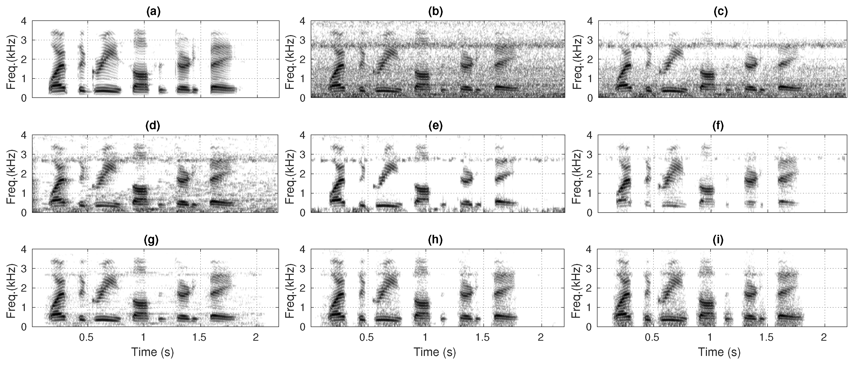
Figure 11 and Figure 12 compare the spectrograms of enhanced speech produced by each SEA for noisy speech data set (Section 4.2). Typically, the noise reduction is visibly improved when going from the KF-non-oracle method to the KF-oracle method. Specifically, the biased gain of the KF-non-oracle method passes a significant residual noise in the enhanced speech (Figure 11c and Figure 12c). Additionally, the poor estimates of the a priori SNR introduces a high degree of residual noise in the enhanced speech produced by the MMSE-STSA method [9] (Figure 11d and Figure 12d). The degree of residual noise decreases in the enhanced speech produced by the AKF-IT method [13] (Figure 11e and Figure 12e). However, the residual noise appears as musical noise. The enhanced speech also gets distorted due to processing the noisy speech iteratively by AKF. The AKF-RMBT method [22] exhibits less residual noise in the enhanced speech; however, it suffers from distortion due to the underestimated Kalman gain (Figure 11f and Figure 12f). The MDKF-MMSE method [17] produces less distorted speech (Figure 11g and Figure 12g) as compared to AKF-RMBT method (Figure 11f and Figure 12f). It can be seen that the proposed method produces enhanced speech with significantly less residual background noise and speech distortion (Figure 11h and Figure 12h) than MDKF-MMSE [17] (Figure 11g and Figure 12g). In addition, the enhanced speech produced by the proposed method is closely similar to the KF-oracle method (Figure 11i and Figure 12i). It is due to the reduced-biased Kalman gain of the proposed method, which is very similar to that of the KF-oracle method.

5.4. Subjective Evaluation by AB Listening Test

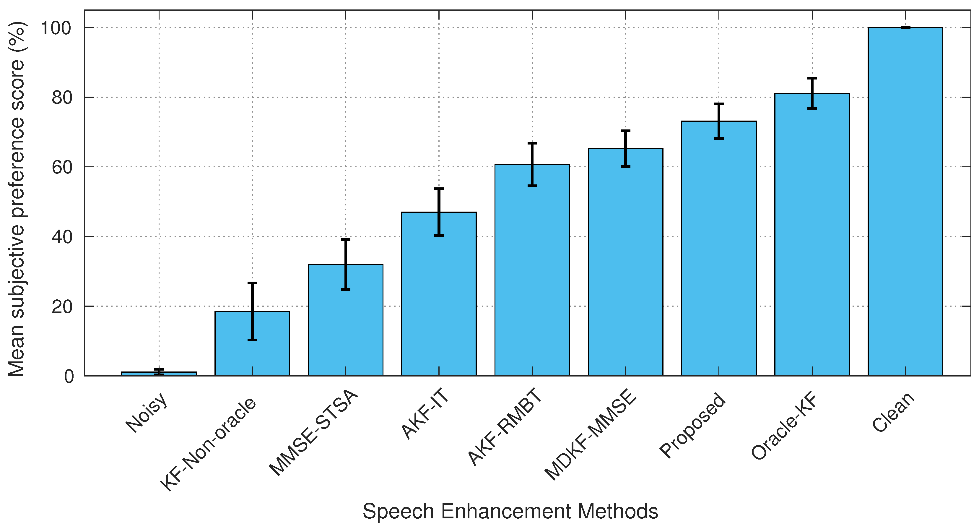
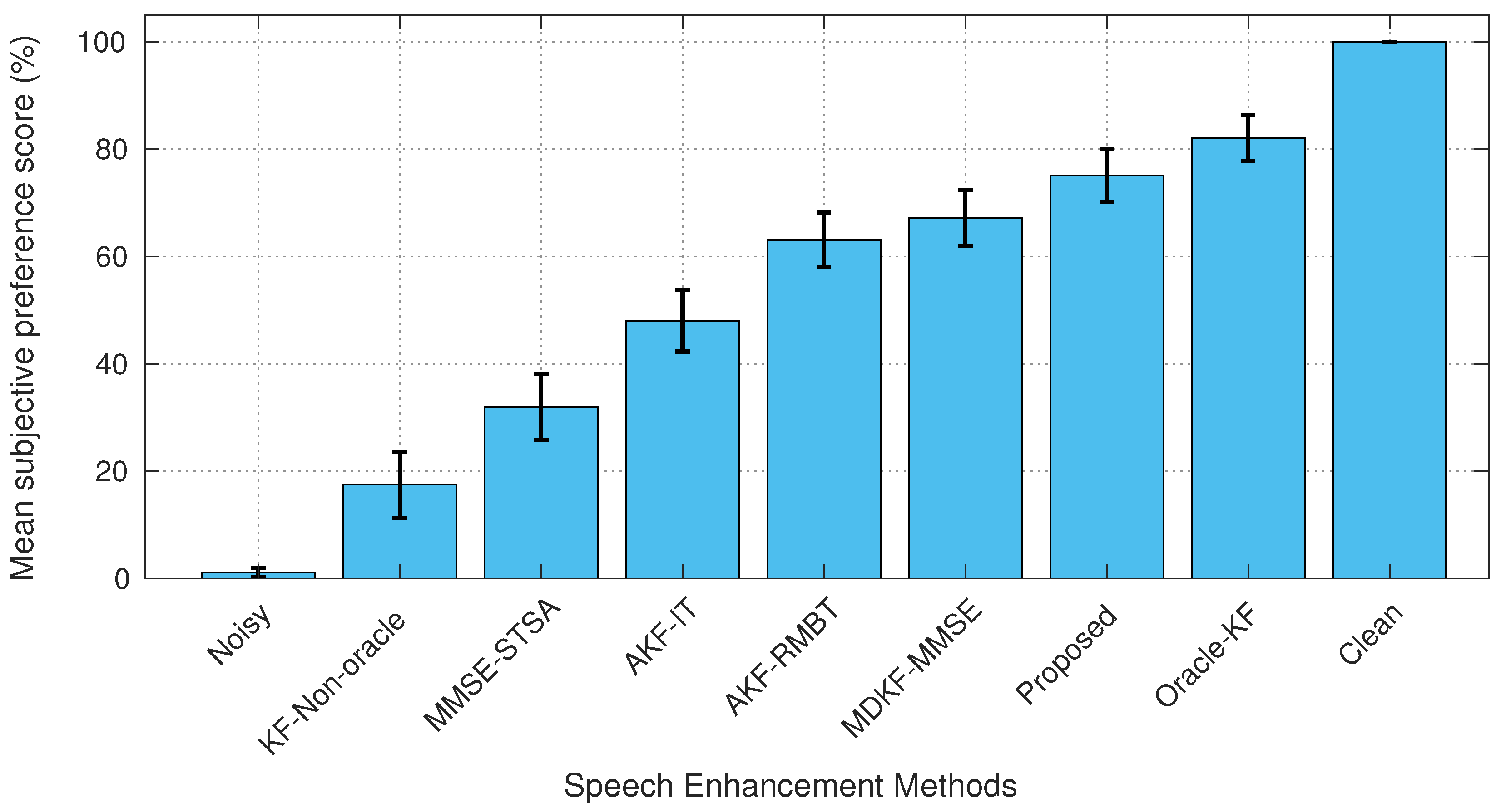
The mean preference score (%) comparisons for all methods are shown in Figure 13 and Figure 14. The non-stationary (babble) noise experiment in Figure 13 reveals that the proposed method is widely preferred (73%) by the listeners to that of the benchmark methods, apart from the clean speech (100 %) and the KF-oracle method (81%). Amongst the benchmark methods, MDKF-MMSE [17] is most preferred (65%) with AKF-RMBT [22] (60%). Although the AKF-IT [22] produced distorted speech, as confirmed by objective PESQ, SDR, and STOI score comparison as well as spectrogram analysis, the listeners prefer it (47%) over MMSE-STSA [9] (31%). The subjective testing implies that it was considered as an improvement of noise reduction in the speech region than a distortion. The colored (f16) noise experiment (Figure 14) also confirms that the proposed method achieves a significant preference score (75%) compared to the benchmark methods, excepting the clean speech (100%) and the KF-oracle method (82%). Among the benchmark methods, MDKF-MMSE [17] is found to be the most preferred (67%) with AKF-RMBT [22] (63%). In light of the blind AB listening tests, it is evident that the enhanced speech produced by the proposed method ensures the best perceived quality amongst all tested methods for both male and female utterances corrupted by real-life non-stationary as well as colored noises.

6. Conclusions

Robustness and sensitivity metric-based tuning of the Kalman filter gain for single-channel speech enhancement has been investigated in this paper. At first, the noise variance was computed from the estimated noise for each noisy speech frame using a speech presence probability method. A whitening filter was also constructed to pre-whiten each noisy speech frame prior to computing LPC parameters. Then, the robustness and the sensitivity metrics were incorporated differently depending on the speech activity of the noisy speech to dynamically offset the bias in Kalman gain. The noise variance and the AR model parameters were adopted as a speech activity detector. It is shown that the proposed tuning algorithm yields a significant reduced-biased Kalman gain, which enables the KF to minimize the residual noise and distortion in the enhanced speech. Extensive objective and subjective scores on the NOIZEUS corpus demonstrate that the proposed method outperforms the benchmark methods in real-life noise conditions for a wide range of SNR levels.

References

- Loizou, P.C. Speech Enhancement: Theory and Practice, 2nd ed.; CRC Press Inc.: Boca Raton, FL, USA, 2013. [Google Scholar]
- Boll, S. Suppression of acoustic noise in speech using spectral subtraction. IEEE Trans. Acoust. Speech Signal Process. 1979, 27, 113–120. [Google Scholar] [CrossRef] [Green Version]
- Berouti, M.; Schwartz, R.; Makhoul, J. Enhancement of speech corrupted by acoustic noise. In Proceedings of the IEEE International Conference on Acoustics, Speech, and Signal Processing, Washington, DC, USA, 2–4 April 1979; Volume 4, pp. 208–211. [Google Scholar] [CrossRef] [Green Version]
- Kamath, S.; Loizou, P. A Multi-Band Spectral Subtraction Method for Enhancing Speech Corrupted by Colored Noise. In Proceedings of the 2002 IEEE International Conference on Acoustics, Speech, and Signal Processing, Orlando, FL, USA, 13–17 May 2002; Volume 4, pp. 4160–4164. [Google Scholar] [CrossRef]
- Paliwal, K.; Wójcicki, K.; Schwerin, B. Single-channel Speech Enhancement Using Spectral Subtraction in the Short-time Modulation Domain. Speech Commun. 2010, 52, 450–475. [Google Scholar] [CrossRef]
- Lim, J.S.; Oppenheim, A.V. Enhancement and bandwidth compression of noisy speech. Proc. IEEE 1979, 67, 1586–1604. [Google Scholar] [CrossRef]
- Scalart, P.; Filho, J.V. Speech enhancement based on a priori signal to noise estimation. In Proceedings of the IEEE International Conference on Acoustics, Speech, and Signal Processing Conference Proceedings, Atlanta, GA, USA, 9 May 1996; Volume 2, pp. 629–632. [Google Scholar]
- Plapous, C.; Marro, C.; Mauuary, L.; Scalart, P. A two-step noise reduction technique. In Proceedings of the IEEE International Conference on Acoustics, Speech, and Signal Processing, Montreal, QC, Canada, 17–21 May 2004; Volume 1, pp. 289–292. [Google Scholar]
- Ephraim, Y.; Malah, D. Speech enhancement using a minimum-mean square error short-time spectral amplitude estimator. IEEE Trans. Acoust. Speech Signal Process. 1984, 32, 1109–1121. [Google Scholar] [CrossRef] [Green Version]
- Ephraim, Y.; Malah, D. Speech enhancement using a minimum mean-square error log-spectral amplitude estimator. IEEE Trans. Acoust. Speech Signal Process. 1985, 33, 443–445. [Google Scholar] [CrossRef]
- Paliwal, K.; Schwerin, B.; Wójcicki, K. Speech enhancement using a minimum mean-square error short-time spectral modulation magnitude estimator. Speech Commun. 2012, 54, 282–305. [Google Scholar] [CrossRef]
- Paliwal, K.; Basu, A. A speech enhancement method based on Kalman filtering. In Proceedings of the IEEE International Conference on Acoustics, Speech, and Signal Processing, Dallas, TX, USA, 6–9 April 1987; Volume 12, pp. 177–180. [Google Scholar] [CrossRef]
- Gibson, J.D.; Koo, B.; Gray, S.D. Filtering of colored noise for speech enhancement and coding. IEEE Trans. Signal Process. 1991, 39, 1732–1742. [Google Scholar] [CrossRef]
- Wang, Y.; Wang, D. Towards Scaling Up Classification-Based Speech Separation. IEEE Trans. Audio Speech Lang. Process. 2013, 21, 1381–1390. [Google Scholar] [CrossRef] [Green Version]
- Xu, Y.; Du, J.; Dai, L.; Lee, C. An Experimental Study on Speech Enhancement Based on Deep Neural Networks. IEEE Signal Process. Lett. 2014, 21, 65–68. [Google Scholar] [CrossRef]
- Williamson, D.S.; Wang, Y.; Wang, D. Complex Ratio Masking for Monaural Speech Separation. IEEE/ACM Trans. Audio Speech Lang. Process. 2016, 24, 483–492. [Google Scholar] [CrossRef] [Green Version]
- So, S.; Paliwal, K.K. Modulation-domain Kalman filtering for single-channel speech enhancement. Speech Commun. 2011, 53, 818–829. [Google Scholar] [CrossRef]
- Roy, S.K.; Zhu, W.P.; Champagne, B. Single channel speech enhancement using subband iterative Kalman filter. In Proceedings of the IEEE International Symposium on Circuits and Systems (ISCAS), Montreal, QC, Canada, 22–25 May 2016; pp. 762–765. [Google Scholar] [CrossRef]
- Saha, M.; Ghosh, R.; Goswami, B. Robustness and Sensitivity Metrics for Tuning the Extended Kalman Filter. IEEE Trans. Instrum. Meas. 2014, 63, 964–971. [Google Scholar] [CrossRef]
- So, S.; George, A.E.W.; Ghosh, R.; Paliwal, K.K. A non-iterative Kalman filtering algorithm with dynamic gain adjustment for single-channel speech enhancement. Int. J. Signal Process. Syst. 2016, 4, 263–268. [Google Scholar] [CrossRef]
- So, S.; George, A.E.W.; Ghosh, R.; Paliwal, K.K. Kalman Filter with Sensitivity Tuning for Improved Noise Reduction in Speech. Circuits Syst. Signal Process. 2017, 36, 1476–1492. [Google Scholar] [CrossRef]
- George, A.E.; So, S.; Ghosh, R.; Paliwal, K.K. Robustness metric-based tuning of the augmented Kalman filter for the enhancement of speech corrupted with coloured noise. Speech Commun. 2018, 105, 62–76. [Google Scholar] [CrossRef]
- Vaseghi, S.V. Linear prediction models. In Advanced Digital Signal Processing and Noise Reduction; John Wiley & Sons: Hoboken, NJ, USA, 2009; Chapter 8; pp. 227–262. [Google Scholar]
- Varga, A.; Steeneken, H.J. Assessment for automatic speech recognition: II. NOISEX-92: A database and an experiment to study the effect of additive noise on speech recognition systems. Speech Commun. 1993, 12, 247–251. [Google Scholar] [CrossRef]
- Oppenheim, A.V.; Schafer, R.W. Discrete-Time Signal Processing, 3rd ed.; Prentice Hall Press: Upper Saddle River, NJ, USA, 2009. [Google Scholar]
- Gerkmann, T.; Hendriks, R.C. Unbiased MMSE-Based Noise Power Estimation With Low Complexity and Low Tracking Delay. IEEE Trans. Audio Speech Lang. Process. 2012, 20, 1383–1393. [Google Scholar] [CrossRef]
- Pearce, D.; Hirsch, H. The aurora experimental framework for the performance evaluation of speech recognition systems under noisy conditions. In Proceedings of the Sixth International Conference on Spoken Language Processing, ICSLP 2000/INTERSPEECH 2000, Beijing, China, 16–20 October 2000; pp. 29–32. [Google Scholar]
- Rix, A.W.; Beerends, J.G.; Hollier, M.P.; Hekstra, A.P. Perceptual evaluation of speech quality (PESQ)—A new method for speech quality assessment of telephone networks and codecs. In Proceedings of the IEEE International Conference on Acoustics, Speech, and Signal Processing (Cat. No.01CH37221), Salt Lake City, UT, USA, 7–11 May 2001; Volume 2, pp. 749–752. [Google Scholar] [CrossRef]
- Vincent, E.; Gribonval, R.; Fevotte, C. Performance measurement in blind audio source separation. IEEE Trans. Audio Speech Lang. Process. 2006, 14, 1462–1469. [Google Scholar] [CrossRef] [Green Version]
- Taal, C.H.; Hendriks, R.C.; Heusdens, R.; Jensen, J. An Algorithm for Intelligibility Prediction of Time–Frequency Weighted Noisy Speech. IEEE Trans. Audio Speech Lang. Process. 2011, 19, 2125–2136. [Google Scholar] [CrossRef]
Figure 1.
Review of existing KF-based SEA: (a,b) spectrograms of the clean speech (utterance sp05) and the noisy speech (corrupt (a) with 5 dB WGN), (c) and metrics, (d) oracle and non-oracle with adjusted and , spectrogram of enhanced speech produced by: (e) KF-oracle method, (f) KF-non-oracle method, (g,h) methods in [20,21].
Figure 2.
Biasing effect of : (a,b) spectrograms of the clean speech and the noisy speech (corrupt sp05 with 5 dB babble noise), (c) computed in oracle and non-oracle cases, (d,e) and computed in oracle and non-oracle cases, (f) and computed from the noisy speech in (b), spectrogram of enhanced speech produced by: (g) KF-oracle method and (h) KF-non-oracle method.
Figure 3.
Block diagram of the proposed KF-based SEA.
Figure 4.
Comparing the estimated: (a) , and (b) , metrics from the noisy speech in Figure 2c.
Figure 5.
Comparing the detected flags of Figure 2b to that of the reference corresponding to Figure 2a.
Figure 6.
responses in terms of: (a) and , and (b) and , where the same experimental setup of Figure 2b is used.
Figure 7.
Comparing obtained using KF-pracle, proposed, and AKF-RMBT [22] methods from the utterance sp05 corrupted with 5 dB: (a) non-stationary (babble) and (b) colored (f16) noises.
Figure 8.
Average PESQ score comparison between the proposed and benchmark SEAs on NOIZEUS corpus corrupted with: (a) babble, (b) street, (c) factory2, and (d) f16 noises for a wide range of SNR levels (from −5 to 15 dB).
Figure 9.
Average SDR (dB) score comparison between the proposed and benchmark SEAs on NOIZEUS corpus corrupted with: (a) babble, (b) street, (c) factory2, and (d) f16 noises for a wide range of SNR levels (from −5 to 15 dB).
Figure 10.
Average STOI score comparison between the proposed and benchmark SEAs on NOIZEUS corpus corrupted with: (a) babble, (b) street, (c) factory2, and (d) f16 noises for a wide range of SNR levels (from −5 dB to 15 dB).
Figure 11.
Comparing the spectrograms of: (a) clean speech (utterance sp05), (b) noisy speech (corrupt sp05 with 5 dB babble noise) (PESQ = 2.10), enhanced speech produced by the: (c) KF-non-oracle (PESQ = 2.18), (d) MMSE-STSA [9] (PESQ = 2.32), (e) AKF-IT [13] (PESQ = 2.26), (f) AKF-RMBT [22] (PESQ = 2.42), (g) MDKF-MMSE (PESQ = 2.48), (h) proposed (PESQ = 2.55), and (i) KF-nracle (PESQ = 2.61) methods.
Figure 12.
Comparing the spectrograms of: (a) clean speech (utterance sp05), (b) noisy speech (corrupt sp05 with 5 dB f16 noise) (PESQ = 2.14), enhanced speech produced by the: (c) KF-non-oracle (PESQ = 2.26), (d) MMSE-STSA [9] (PESQ = 2.39), (e) AKF-IT [13] (PESQ = 2.31), (f) AKF-RMBT [22] (PESQ = 2.53), (g) MDKF-MMSE (PESQ = 2.58), (h) proposed (PESQ = 2.65), and (i) KF-oracle (PESQ = 2.70) methods.
Figure 13.
The mean preference score (%) comparison between the proposed and benchmark SEAs for the utterance sp05 corrupted with 5 dB non-stationary babble noise.
Figure 14.
The mean preference score (%) comparison between the proposed and benchmark SEAs for the utterance sp27 corrupted with 5 dB colored f16 noise.
Publisher’s Note: MDPI stays neutral with regard to jurisdictional claims in published maps and institutional affiliations. |
© 2021 by the authors. Licensee MDPI, Basel, Switzerland. This article is an open access article distributed under the terms and conditions of the Creative Commons Attribution (CC BY) license (https://creativecommons.org/licenses/by/4.0/).
Share and Cite
MDPI and ACS Style
Roy, S.K.; Paliwal, K.K. Robustness and Sensitivity Tuning of the Kalman Filter for Speech Enhancement. Signals 2021, 2, 434-455. https://0-doi-org.brum.beds.ac.uk/10.3390/signals2030027
AMA Style
Roy SK, Paliwal KK. Robustness and Sensitivity Tuning of the Kalman Filter for Speech Enhancement. Signals. 2021; 2(3):434-455. https://0-doi-org.brum.beds.ac.uk/10.3390/signals2030027
Chicago/Turabian StyleRoy, Sujan Kumar, and Kuldip K. Paliwal. 2021. "Robustness and Sensitivity Tuning of the Kalman Filter for Speech Enhancement" Signals 2, no. 3: 434-455. https://0-doi-org.brum.beds.ac.uk/10.3390/signals2030027