
Adaptive Probabilistic Optimization Approach for Vibration-Based Structural Health Monitoring


1
Department of Engineering, University of Jamestown, 6028 College Lane, Jamestown, ND 58405, USA
2
School of Engineering and Technology, Western Carolina University, 1 University Way, Cullowhee, NC 28723, USA
*
Author to whom correspondence should be addressed.
Signals 2021, 2(3), 475-489; https://0-doi-org.brum.beds.ac.uk/10.3390/signals2030029
Submission received: 28 April 2021
/
Revised: 19 June 2021
/
Accepted: 9 July 2021
/
Published: 17 July 2021
(This article belongs to the Special Issue Advanced Signal/Data Processing for Structural Health Monitoring)
Abstract
:This paper presents a novel adaptive probabilistic algorithm to identify damage characteristics by integrating the use of the frequency response function with an optimization approach. The proposed algorithm evaluates the probability of damage existence and determines salient details such as damage location and damage severity in a probabilistic manner. A multistage sequence is used to determine the probability of damage parameters including crack depth and crack location while minimizing uncertainties. A simply supported beam with an open edge crack was used to demonstrate the application of the algorithm for damage detection. The robustness of the algorithm was tested by incorporating varying levels of noise into the frequency response. All simulation results show successful detection of damage with a relatively high probability even in the presence of noise. Results indicate that the probabilistic algorithm could have significant advantages over conventional deterministic methods since it has the ability to avoid yielding false negatives that are quite common among deterministic damage detection techniques.
1. Introduction
Over the last few decades, there have been rapid advances in the use of damage diagnostics and damage detection for structural health monitoring (SHM) [1]. These advances have emerged hand-in-hand with the development of sensor technologies and data processing capabilities. The use of damage detection is crucial for the analysis and maintenance of large and complex structural installations with a relatively long lifespan. In the literature, several SHM methods have been developed for damage identification using strain modes, ultrasonic waves, electromechanical impedance, frequency response functions, and modal properties such as natural frequencies and mode shapes [2,3,4,5,6,7]. However, most of the techniques presented in the literature have used deterministic models which often exclude elements of uncertainty and variability that are inherent in environmental conditions and measurements.
The use of the frequency response function (FRF) for damage detection and structural health monitoring has been widespread [8,9,10]. Recently, the use of FRF has been augmented by using artificial neural networks (ANN) and genetic algorithms (GA) for damage detection [11,12,13]. It has been specifically observed that ANN could be used for the detection of nonlinear damage with a high level of accuracy [11]; however, most of the techniques that use ANN require a large amount of training data. Some recent studies have also used machine learning algorithms to detect damage under varying operational and environmental conditions [14]. It is observed that the training data should cover the full range of operational and environmental variability for the successful use of machine learning for damage detection, while developing a capability to identify a dynamic response that is triggered by damage [14]. While FRF has been found to be very useful for damage diagnostics, it is widely acknowledged that signal processing and analysis are critical in structural health monitoring due to the issues associated with sensor noise, measurement inaccuracies, etc. [15]. Furthermore, a large amount of training data is required to capture operational and environmental variability for machine learning algorithms.
Model properties of structures in conjunction with the wavelet transform and optimization methods have also been used by many researchers for damage detection [16]. Wavelet-based methods are frequently used due to their ability to detect local discontinuities or singularities due to small cracks and the associated properties [17,18]. The use of wavelets in the literature includes the use of a global damage sensitivity trait by using the Haar wavelet [19] or the use of a diagnostic technique to identify the magnitude and location of a crack in beams by using skewness and kurtosis of mode shapes [20]. Another algorithm in the literature makes use of Symlets to detect mixed-mode cracks in large warren truss structures by utilizing natural modes [17]; however, the use of coarse sampling in large structures makes it challenging to use such an algorithm to accurately detect the extent and location of damage. In general, it can be stated that mode shape-based methods are highly sensitive to sampling and quality of sensor measurements [18], but the availability of full-field methods such as 3D digital image correlation (3D-DIC) and Continuous-scan laser Doppler vibrometry (CSLDV) have made it possible to measure a large number of velocities and displacements with relatively high accuracy [21,22].
To investigate the sensitivity of overall damage detection to local and global damage, many optimization-based methods have been used in the literature with the aim of minimizing sensor measurements. To demonstrate the robustness and capabilities of these techniques, large and complex structural applications have been tested by using numerical and experimental examples [23,24,25,26]. For instance, particle swarm optimization has been used to develop a multi-stage optimization algorithm that makes use of natural frequencies to detect multiple damages [23]. Damage is specifically detected by studying the relative elastic modulus reduction. A genetic algorithm has also been used to analyze and identify structural damage by comparing the measured vibrational data to data acquired before damage [24]. This approach has been tested on a cantilever beam and some frame structures. While the actual damage was detected accurately in this study, two additional incorrect damage locations were detected [24]. Other methods that have been used for damage detection include the use of an optimum updating method for global damage detection [25] and the use of sensitivity and optimization algorithms [26]. The location and intensity of structural damage have been determined by using the difference between stiffness matrices of an initial undamaged model and a test-adjusted damaged model [25]. The optimization algorithm in the literature uses an objective function that is defined as the difference between calculated and measured frequency responses; this method has been successfully used in a five-degree-of-freedom mechanical system to accurately predict the location and intensity of damage [26]. In general, the optimization-based methods have been observed to detect additional damage in some instances while finding it challenging to detect relatively small amounts of damage.
In summary, the literature on damage detection presents multiple techniques to identify damage location and damage severity with varying levels of sensitivity and robustness. Most of the existing literature, however, presents deterministic results for damage diagnostics. This paper attempts to overcome this limitation by presenting a probabilistic approach with an adaptive algorithm that can be used for damage diagnostics by using the frequency response function. The approach presented in this paper allows an evaluation of the probability of damage characteristics. The adaptive algorithm developed in this study is presented in Section 2, while the analytical model for a beam that was used for damage detection is briefly presented in Section 3. Section 4 presents several simulations that are used to demonstrate the application of the proposed approach, while Section 5 summarizes the main findings and draws overall conclusions.
2. Probabilistic Optimization Algorithm
This section provides a detailed description of the algorithm for damage detection. The proposed algorithm integrates the use of the frequency response function (FRF) with optimization and a probabilistic model to identify the size of damage as well as the location of damage.
The approach presented in this study uses the FRF to identify damage characteristics. The optimization problem is formulated to find the crack depth and crack location ratios by minimizing the difference between the measured FRF and the calculated FRF as follows:
In Equation (1),
is the measured FRF,
is the calculated FRF,
is the crack size ratio,
is the crack location ratio, and
is the absolute difference between the measured and calculated FRFs over the frequency range, for the kth segment. The objective function is minimized by using sequential quadratic programming (SQP), which is an iterative method suitable for constrained nonlinear optimization problems. An extensive amount of detail on SQP can be found in [27]. Prior to this optimization process, the measured FRF signals are de-noised by using the discrete wavelet transform with Daubechies mother wavelet, at level four wavelet decomposition.
The frequency range and the number of samples in each segment are important factors that provide details about damage features and can also affect the confidence level in signal processing outcomes. Smaller segments can typically reveal more information but may be computationally expensive. This trade-off may need to be carefully evaluated when the data are being collected continuously, as is common in structural health monitoring. Thus, the segment size is defined as:
In Equation (2),
is the next segment size,
is the current segment size, N is the minimum segment size, and
is the segment size factor. This factor controls the segment size by increasing or decreasing the number of samples that should be added or subtracted from the next segment depending on the magnitude of
that represents the level of agreement between the measured and calculated FRFs, i.e., the smaller is, the larger the next segment will be. The segment size factor is defined as:
The limits in Equation (3),
and
, may vary from one application to another. The limits can be determined by the user to evaluate the appropriate limits for increasing and decreasing the segment size given the magnitude of error between measured and calculated FRFs. Since the segments vary in size, a weighting factor
is assigned to each segment. Therefore, large segments are associated with large weighting factors, i.e., the larger the segment, the higher the contribution it provides to the analysis of the damage identification process. The calculated FRF is a function of two design variables with upper bounds and lower bounds. By minimizing the objective function for each segment, the algorithm provides two vectors for each design variable. The size of each vector is the same as the number of segments created from the measured FRF.
The algorithm was further developed to optimize the probability of crack location and crack size ratios while minimizing the uncertainty range to less than
and
, respectively, such that
and
have a range of (0,1). For the crack location, the optimization problem is formulated as:
Similarly, the optimization problem for the crack size can be expressed as:
Eventually, these data are further processed to identify the status of a structure in order to determine whether it is undamaged or damaged by using the probabilities of crack location ratio and crack size ratio. The probability of the damage existence is calculated as:
In Equation (6),
is the weighting factor with a range of (0, 1) that is set by the user. The probability of the optimal crack location and its corresponding range contributes
to the probability of damage existence, whereas the probability of crack size ratio contributes to the probability of damage existence. As can be noted from Equation (6), when the range of crack location ratio
is too broad or close to unity, it renders the contribution of crack location to the probability of damage existence to zero. The measured FRF,
, which is used to test the proposed algorithm was generated by adding random noise to the calculated FRF,
, as:
In Equation (7),
is the relative magnitude of error, and ζ is the uniformly distributed pseudorandom vector within the range of (0,1) [28]. This random noise represents different sources of error such as the immediate working environment, instrument resolution, and lack of exact modeling and absolute agreement between the actual structure and simulations. While the noise model used in this study may be simplistic, it allows an investigation of various levels of noise to simulate the worst-case scenario by varying the magnitude of error.
Adaptive Multi-Stage Algorithm
A multi-stage algorithm has been developed for damage detection. The algorithm is summarized in the following steps:
- Import the measured FRF, and set user inputs: , ,
- De-noise using discrete wavelet transform.
- Stage q: Define design variables and their respective constraints.
- Provide an initial guess for each design variable, .
- Set the segment size to , and the weighting factor to .
- Use sequential quadratic programming (SQP) algorithm to minimize the difference between FRFs for kth segment.
- Store the optimal solutions for each design variable in vector.
- Set the size of the next segment to , and repeat steps 3 through 7 until all data are processed.
- Use SQP again to calculate the maximum probability of crack location and crack size, while minimizing the uncertainty range using the data collected in step 7.
- Save the computed crack size and crack location ranges and their respective probabilities.
- Calculate the probability of damage existence, , using the available data of crack size and crack location from step 10.
- Stage q + 1: Update lower and upper bounds as well as the initial guesses in step 4 according to the results from step 10.
- If the probability of damage existence is below a threshold, where is user input, move to step 15.
- Repeat steps 4 through 13.
- Save the optimal crack size and crack location ranges along with their probabilities and report the results.
A flowchart of the algorithm is shown in Figure 1. The proposed algorithm was tested for different damage scenarios for a simply supported beam. Details on damage modeling and results from the algorithm are provided in the subsequent sections.
3. Modeling Method
This section provides a brief description of the analytical model that was used as the baseline for a simply supported beam. More details about the model can be found in the reference literature [29,30,31].
3.1. Analytical Modeling
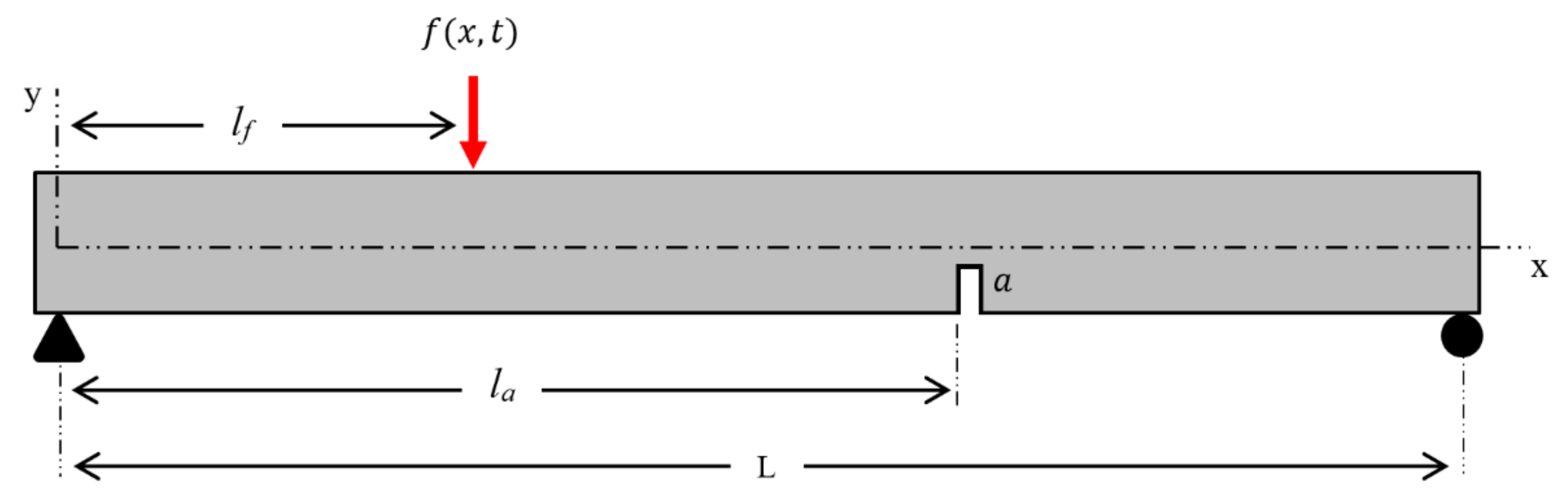
A simply supported beam with an open crack was used to simulate the application of the damage detection algorithm presented in Section 2. The proposed algorithm utilized an optimization technique for detecting damage by using the frequency response. The beam shown in Figure 2 has a transverse crack (with crack length, ) that is located at
. Damage is modeled as a torsional spring between the two sides of the beam. The simply supported beam is subjected to a sinusoidal load with forcing frequency, located at
. Parameters such as crack depth and crack location have been varied to generate several damage cases that were used to evaluate the effectiveness of the proposed algorithm.
The modal properties of a uniform beam can be obtained by using the equation of motion (EOM) derived from the Euler–Bernoulli formulation [29] as follows:
In Equation (8),
is the Young’s modulus of the material,
is the material density,
is the lateral displacement at time
and location ,
is the external load, A is the cross-sectional area of the beam, and I is the moment of inertia. The system response is determined by finding the steady-state solution and the transient solution of the beam. The general solution of Equation (8) including the steady-state solution as well as the particular solution,
, is:
The coefficients,
in Equations (9) and (10) can be determined by applying the boundary conditions and the compatibility conditions. The frequency response function is defined as the ratio of the output amplitude, to the input amplitude
. Therefore, the frequency response function is expressed as:
3.2. Damage Modeling
Using linear elastic fracture mechanics, an edge crack is simulated by a non-dimensional compliance,
. The non-dimensional compliance was used to model the local flexibility in the form of a torsional spring. It is defined as:
In Equation (12), Kt is the torsional stiffness of an opening crack under a bending load. Since the ratio of the beam length to the lateral length is large, it can be assumed that the contribution of mode-II to the total strain energy is negligible as compared to the contribution of mode-I. Thus, only the opening mode is considered for analysis. The local flexibility is captured by calculating the change in strain energy near the crack tip [30] and can expressed as:
In Equation (10),
is the non-dimensional geometrical factor, and
is the relative crack size, defined as the ratio between the crack size, a, and the beam height,
. The non-dimensional factor for an opening mode crack is determined empirically [31] as follows:
It may be noted the FRF of an undamaged beam can be obtained by setting the non-dimensional compliance to zero.
4. Results and Discussion
Three damage cases of a simply supported beam with different characteristics and different levels of noise have been considered to evaluate the effectiveness of the probabilistic optimization algorithm. The details of the three cases are provided in Table 1.
User inputs for the adaptive algorithm are listed in Table 2. The user input values are subject to change and could vary with applications of interest, quality of measurements, and the precision required in the detection of damage characteristics. The segment size limits in Equation (3) are set to 0.1 and 0.5 for
and
, respectively. Thus, the segment size increases when the absolute difference between measured and calculated FRFs,
, is less than 0.1, and decreases when
is greater than 0.5.
The probability constraints in Equations (4) and (5) are set to 15%. This implies that the probabilities of crack size ratio and crack location ratio are optimized such that the predicted values are within 15% of the beam dimensions. A 60% weighting factor is assigned to
in Equation (6) for the probability of damage existence. This implies that the probability of crack location contributes 60% to the probability of damage existence and the remaining 40% is assigned to the probability of non-zero crack size. The adaptive algorithm is set to terminate when the difference between the current stage probability of damage existence
and the previous stage probability
is less than 5%. For the sake of simplicity, algorithm results were limited to two stages only for each case considered in the study.
The beam used for analysis made of aluminum has a rectangular cross-section with a length of
mm and cross-sectional dimensions of 5 mm
10 mm. A Young’s modulus of 70 GPa and a density of 2800 kg/m3 are used for analysis. The forcing frequency range for each case was kept unchanged throughout the analysis. The excitation force has a frequency ranging from 1 Hz to 32 Hz. Similarly, the applied force is located at 300 mm from the left end of the beam. The random noise level that is added to the simulated frequency response is increased from Case 1 to Case 3, using 1%, 9%, and 15%, respectively. Figure 3 shows the frequency response signal collected from a node located at 350 mm from the origin.
Case 1
In Case 1, a 3 mm open crack () was inflicted in the simply supported beam at 400 mm from the left boundary, as shown in Figure 2. The frequency response signal was collected from a node located at 350 mm. The proposed algorithm provided salient information about the damage characteristics in terms of damage location and severity. Table 3 shows the adaptive algorithm outputs including the probability of damage existence, probability of crack size, and probability of crack location for each stage. In stage 1, the algorithm predicted the existence of damage with a probability of 66.1%. The depth of the crack was predicted to be between 6.33 mm and 6.93 mm with an approximately 50% probability. The predicted crack size was more than twice the actual crack size. However, the crack location was predicted within 20 mm of the damage location with a 55% probability.
The frequency diagrams of crack size and crack location for two stages are plotted in Figure 4. The y-axis represents the number of occurrences, n. The frequency diagram of crack location suggests that the crack location is within ±40 mm range from 450 mm. In stage 1, however, the frequency diagram of crack size in Figure 4b indicates that there were three potential crack depths with average values of 0.5 mm, 3 mm, and 6.5 mm. The optimal range of crack size reported by the algorithm represents the occurrences falling within that range, making 6.5 mm a strong candidate in stage 1.
In stage 2, the algorithm yielded a significant improvement in the probabilities and the predicted ranges for crack size and crack location. As can be seen from Table 3, the probability of damage existence increased to about 89%. The actual crack location was detected with a high probability. The damage was predicted between 377 mm and 408 mm with a probability of 90.7%. Crack location range increased slightly from 2.2% in stage 1 to 3.1% of the beam length in stage 2. However, the range remained within the design constraint (), which was set at 15% of the beam length. The probability improved significantly, and the actual crack location was included within the predicted range in stage 2. The probability of crack size also improved by more than 20%, and the predicted crack size was much closer to the actual value.
It is worth noting that the frequency diagrams for both stages in Figure 4b show no occurrences of crack size greater than 7.5 mm, as well as other smaller ranges around 1.5 mm and 4.5 mm. Likewise, all occurrences of damage location in both stages fell between 300 mm and 450 mm. This demonstrates that the adaptive algorithm can also be used to eliminate regions that might be less likely to be damaged and consequently assist in directing inspection resources to more likely regions of expected areas. Limiting potential solutions to a few scenarios is an appreciable advantage of the probabilistic approach over the deterministic approach.
This case was repeated with the same damage characteristics and zero noise. The results which were not included here yielded the exact crack location and crack size as the predefined values in the simulation model with about 100% probability. Furthermore, several trials of this case have been repeated with a noise level of 30%. The probability of damage existence was never reported below 53%. Similarly, the actual position of damage was within the predicted range of crack location for most trials. The crack size, however, was consistently underestimated.
Case 2
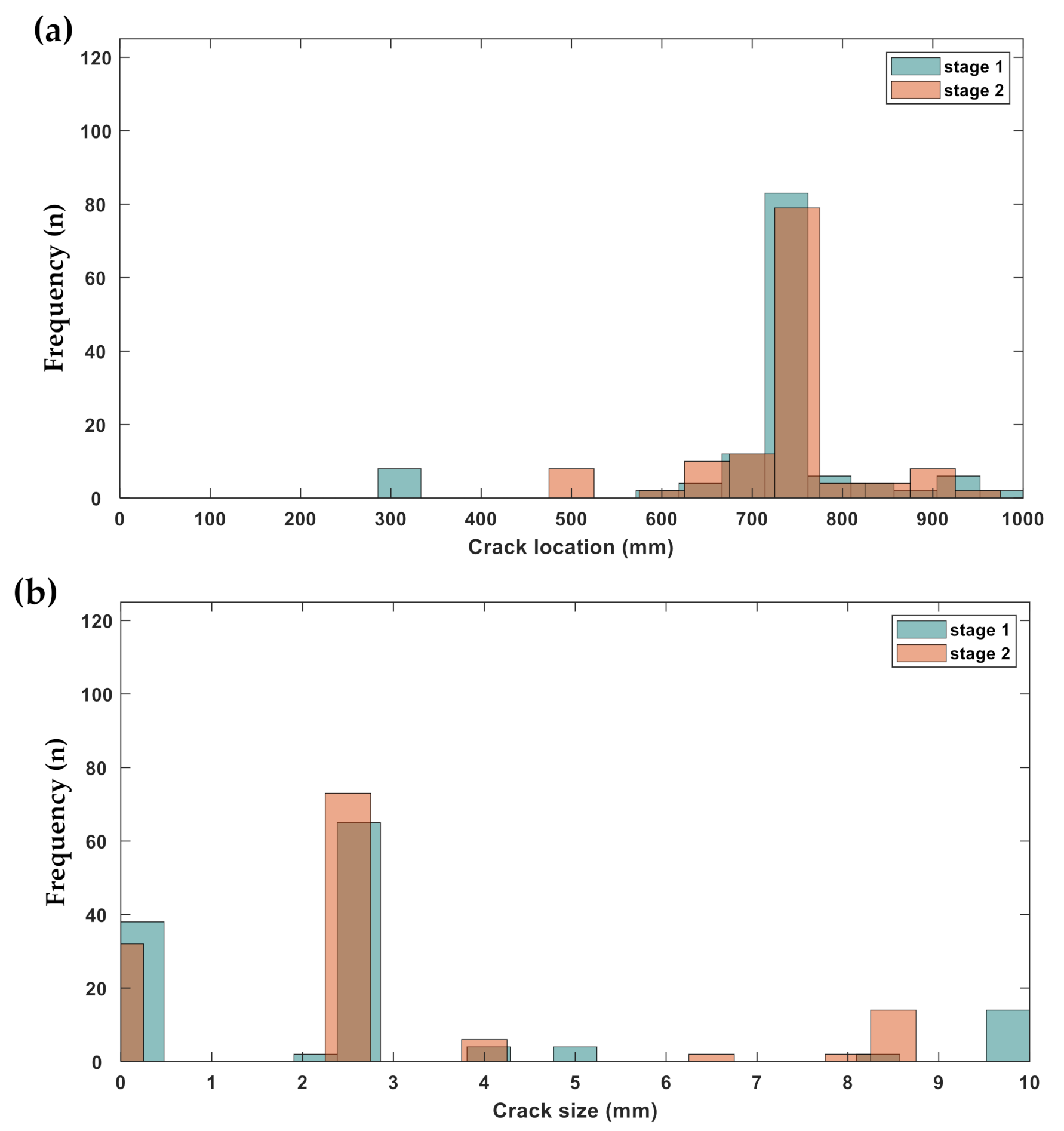
In this case, the noise level was increased to 9% and the crack size was kept unchanged at 30% of the beam thickness. The crack was introduced closer to the left boundary at 725 mm from the origin. The sensor location was moved to the middle of the beam, i.e., data collected from a node located at 500 mm with the crack size being 30% of the beam thickness. The results of the adaptive algorithm are summarized in Table 4.
The results in Table 4 strongly suggest that the simply supported beam is damaged with a probability of approximately 66% at a location between 713 mm and 831 mm. There was a noticeable reduction in the probability of damage existence in comparison to Case 1, which could be attributed to the increase in the level of noise and the locations of damage. The sensor location also was expected to have a significant impact on the analysis of damage identification, which is a research topic that has been pursued by many researchers [32,33,34]. The crack size range in stage 2 was underestimated and slightly below the actual value, and the probability saw a moderate increase of about 3%. On the contrary, the ranges of crack location predicted by the algorithm in both stages included the actual crack position, but the probability sustained a drop of approximately 5%, resulting in a decrease in the probability of damage existence in stage 2.
The predicted range of crack size was about 5% of the beam thickness. However, the crack location in stage 2 was further shifted to the right and the actual crack location moved closer to the lower bound of the predicted range. It can be concluded that the algorithm produced less favorable results in stage 2, especially for crack location with a drop in the probability accompanied by an increase in the predicted range. Given that the algorithm was designed to yield the most probable scenario rather than optimization of the probability of damage, this behavior may be considered to be realistic for a structural health monitoring system. Despite a decline in the probability of damage existence in stage 2, all parameters have been reported with a probability greater than 50% indicating the structure could potentially be damaged.
In Figure 5, the frequency diagrams of crack size and crack location from both stages are superimposed. The 9% noise added to the signal has introduced short side bars spread out around the main bars in the frequency diagrams of crack location. Despite a small drop in the probability of damage location as reported in Table 4, it is worth noting from Figure 5a that the algorithm yields better results for damage location by virtually limiting 100% of occurrences within 50% of the beam length. Likewise, the frequency diagrams of crack size in Figure 5b show noticeable improvements in stage 2 with a higher peak around 2.5 mm and a significant reduction of occurrences at both extremes. Finding a false negative in damage detection is quite common from deterministic methods because damage detection is an ill-posed problem with no unique solution, making a probabilistic approach more appropriate to provide meaningful results in such problems. Despite several damage scenarios presented in Figure 5, the algorithm successfully determined the optimal solution representing the status of the structure.
Case 3
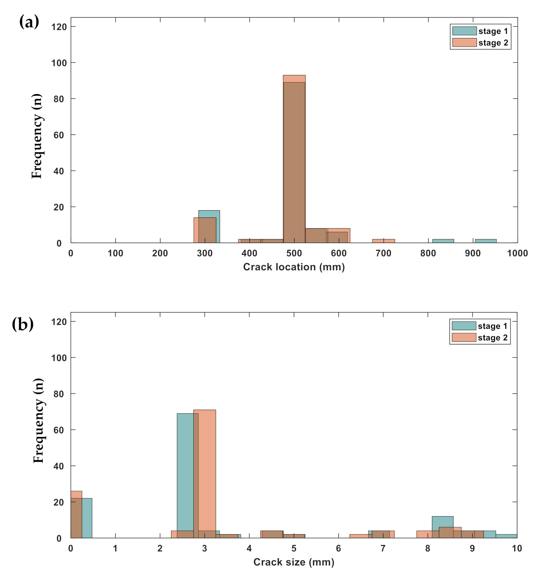
This case further examines the ability of the adaptive optimization approach developed herein to provide probabilistic details for damage characteristics in a simply supported beam. A noise of 15% was introduced into the simulated frequency response of a damaged beam with a smaller crack of 2.8 mm inflicted at the middle of the beam. To avoid overlap of damage and sensor locations, the frequency response data were collected from a node at 350 mm, identical to the sensor location of Case 1. A direct comparison can be made between the two cases due to the sensor location. The results of both stages for Case 3 are presented in Table 5.
As can be seen from the results in Table 5, the probability of damage existence is more than 70% in both stages. This percentage is significant enough to declare the status of the damage. The algorithm successfully predicted the range of the crack size between 2.2 mm and 2.9 mm with the actual crack size being within the predicted range, but the range was slightly shifted and increased in stage 2. However, the algorithm improved the probability of crack size noticeably in the second stage to 55% and the probability of crack location increased to more than 78%. The ranges of crack location were also predicted within the design constraints of 15%.
The probability distributions shown in Figure 6 provide meaningful details about damage characteristics even in the presence of significant noise while the crack size is relatively small. Despite the modest improvement observed in Figure 6a, several occurrences for damage location beyond 800 mm were eliminated in stage 2, with most occurrences predicted within ±100 mm range from the actual damage location. In Figure 6b, there are three potential crack sizes substantially apart in value at about: 0.25 mm, 3 mm, and 8.5 mm. However, the candidate solution calculated by the algorithm was in the vicinity of 3 mm. The algorithm has made a major shift of the 3 mm peak with a minor increase in the number of occurrences. In order to test the algorithm’s ability to predict undamaged status, this case was repeated with no damage. In this case, the adaptive algorithm yielded a crack size of nearly zero with about 90% probability.
It should be noted that the sensor location must be carefully identified in order to avoid vibrational nodes, especially when high frequencies are being considered. Sensor location plays a significant role in accuracy and precision during structural health monitoring. Sensor placement is often informed by several factors, including system dynamics, types of expected defects, number and type of sensors, etc. Given the extensive attention that this topic has received in recent years, several optimization techniques for optimal sensor placement have been devised and applied to various engineering applications [35,36]. It is expected that augmenting this algorithm with an optimal sensor location approach could have positive implications, especially when dealing with complex structures. The results produced herein have been collected from a single sensor. Thus, integrating the proposed approach with a data fusion technique to process data from multiple sensors and sources to produce more accurate, consistent, and useful information about incipient damage in structures is necessary to develop a robust tool for SHM systems.
Computational Time
The adaptive probabilistic algorithm involved employing the SQP to calculate the crack size and crack location in a form of vectors. This step was found to account for the majority of the computational iterations performed by the algorithm, and the average number of iterations for all cases was about 600. The number of iterations was found to be directly related to the level of noise added to the frequency response. In Case 3, the number of iterations reached 830, while the number of iterations for Case 1 was limited to 320. Other signal processes such as those in which SQP was used to minimize the probability of crack location and crack size only accounted for a relatively small percentage of the total computations. Figure 7 shows a summary of the computational time of all the cases considered in the study.
The mean and standard deviation of computational time and probability of damage existence is shown in Table 6 and were calculated for ten trials of each case. In Case 1, the computational time of stage 1 was largely consumed by SQP and was moderately higher for stage 2. This may be related to the significant improvement in the results achieved by the algorithm for the probability of damage existence as reported in Table 6. Additionally, there was a substantial reduction in the standard deviation of the probability of damage existence in stage 2 by about 10%. The algorithm, in Case 2, consumed higher computational time in stage 1 and reported a lower probability of damage existence in stage 2. The mean and standard deviation of computational time for Case 3 were reported relatively close, with a slight improvement in the probability of damage existence in stage 2.
The analysis presented herein was performed by limiting the number of optimization stages in the algorithm to two. The results strongly suggest that two stages may be sufficient for the application investigated in this paper. However, it may be necessary to consider the proposed algorithm with multiple stages for other structural applications.
5. Summary and Future Work
An adaptive damage detection algorithm has been presented in this paper to identify damage characteristics by using the frequency response function. The main conclusions from this study can be summarized as follows:
- The algorithm has been specifically used to calculate the probability of damage existence along with the probabilities associated with the crack size, as well as crack location.
- The adaptive algorithm developed in this study has been evaluated for robustness through three simulated cases with various damage characteristics and different levels of noise.
- In all three cases, the algorithm has been successful in predicting damage even in the presence of a high level of noise and even for relatively small damage.
Multiple variables associated with the algorithm such as the weighting factor, constraint levels, etc. can be established by the user based on prior data or experience with the structure that is being evaluated for SHM. It should be mentioned that this study has been limited to the use of the frequency response data from a single location on a simply supported beam with only one type of defect. Future work will include the application of the probabilistic algorithm that has been developed in this study to large and complex truss and frame structures, as well as structures made of composite materials. Other common types of defects such as disbonds, kissing bonds, voids, and delamination will also be investigated in the future. Since sensor location is expected to play a substantial role in the identification of damage characteristics, sensor placement will be integrated into the framework of the proposed algorithm in future studies.
Author Contributions
Conceptualization, H.A. and S.K.; methodology, H.A. and S.K.; software, H.A.; validation, H.A.; formal analysis, H.A.; investigation, H.A. and S.K.; data curation, H.A.; writing—original draft preparation, H.A. and S.K.; writing—review and editing, H.A. and S.K. All authors have read and agreed to the published version of the manuscript.
Funding
This research received no external funding.
Conflicts of Interest
The authors declare no conflict of interest.
References
- Gholizadeh, S. A review of non-destructive testing methods of composite materials. Procedia Struct. Integr. 2016, 1, 50–57. [Google Scholar] [CrossRef] [Green Version]
- Ghosh, T.; Kundu, T.; Karpur, P. Efficient use of Lamb modes for detecting defects in large plates. Ultrasonics 1998, 36, 791–801. [Google Scholar] [CrossRef]
- Altammar, H.; Dhingra, A.; Salowitz, N. Initial study of internally embedded shear-mode piezoelectric transducers for the detection of joint defects in laminate structures. J. Intell. Mater. Syst. Struct. 2019, 30. [Google Scholar] [CrossRef]
- Poddar, B.; Giurgiutiu, V. Scattering of Lamb waves from a discontinuity: An improved analytical approach. Wave Motion 2016, 65, 79–91. [Google Scholar] [CrossRef]
- Carrison, P.; Altammar, H.; Salowitz, N. Selective actuation and sensing of antisymmetric ultrasonic waves using shear-deforming piezoelectric transducers. Struct. Health Monit. 2021, 20, 978–989. [Google Scholar] [CrossRef]
- Chua, C.A.; Cawley, P. Crack growth monitoring using fundamental shear horizontal guided waves. Struct. Health Monit. 2020, 19, 1311–1322. [Google Scholar] [CrossRef]
- Altammar, H.; Dhingra, A.; Salowitz, N. Ultrasonic Sensing and Actuation in Laminate Structures Using Bondline-Embedded d35 Piezoelectric Sensors. Sensors 2018, 18, 3885. [Google Scholar] [CrossRef] [PubMed] [Green Version]
- Li, B.; Chen, X.F.; Ma, J.X.; He, Z.J. Detection of crack location and size in structures using wavelet finite element methods. J. Sound Vib. 2005, 285, 767–782. [Google Scholar] [CrossRef]
- Trendafilova, I.; Cartmell, M.P.; Ostachowicz, W. Vibration-based damage detection in an aircraft wing scaled model using principal component analysis and pattern recognition. J. Sound Vib. 2008, 313, 560–566. [Google Scholar] [CrossRef] [Green Version]
- Yan, W.J.; Zhao, M.Y.; Sun, Q.; Ren, W.X. Transmissibility-based system identification for structural health Monitoring: Fundamentals, approaches, and applications. Mech. Syst. Signal. Process. 2019, 117, 453–482. [Google Scholar] [CrossRef]
- Bandara, R.P.; Chan, T.H.; Thambiratnam, D.P. Structural damage detection method using frequency response functions. Struct. Health Monit. 2014, 13, 418–429. [Google Scholar] [CrossRef]
- Neves, A.C.; González, I.; Leander, J.; Karoumi, R. Structural health monitoring of bridges: A model-free ANN-based approach to damage detection. J. Civ. Struct. Health Monit. 2017, 7, 689–702. [Google Scholar] [CrossRef] [Green Version]
- Sulaiman, M.S.A.; Yunus, M.A.; Bahari, A.R.; Abdul Rani, M.N. Identification of damage based on frequency response function (FRF) data. MATEC Web Conf. 2016, 90. [Google Scholar] [CrossRef] [Green Version]
- Figueiredo, E.; Park, G.; Farrar, C.R.; Worden, K.; Figueiras, J. Machine learning algorithms for damage detection under operational and environmental variability. Struct. Health Monit. 2011, 10, 559–572. [Google Scholar] [CrossRef]
- Amezquita-Sanchez, J.P.; Adeli, H. Signal Processing Techniques for Vibration-Based Health Monitoring of Smart Structures. Arch. Comput. Methods Eng. 2016, 23, 1–15. [Google Scholar] [CrossRef]
- Doebling, S.W.; Farrar, C.R.; Prime, M.B. A summary review of vibration-based damage identification methods. Shock Vib. Dig. 1998, 30, 91–105. [Google Scholar] [CrossRef] [Green Version]
- Altammar, H.; Kaul, S.; Dhingra, A.K. Use of wavelets for damage diagnostics in truss structures. Int. J. Struct. Integr. 2017, 8, 373–391. [Google Scholar] [CrossRef]
- Fan, W.; Qiao, P. Vibration-based damage identification methods: A review and comparative study. Struct. Health Monit. 2010, 10, 83–111. [Google Scholar] [CrossRef]
- Krishnan Nair, K.; Kiremidjian, A.S.; Nair, K.K.; Kiremidjian, A.S. Derivation of a damage sensitive feature using the haar wavelet transform. J. Appl. Mech. Trans. ASME 2009, 76, 1–9. [Google Scholar] [CrossRef]
- Kaul, S. Crack diagnostics in beams using wavelets, kurtosis and skewness. Nondestruct. Test. Eval. 2014. [Google Scholar] [CrossRef]
- Ehrhardt, D.A.; Yang, S.; Beberniss, T.J.; Allen, M.S. Mode shape comparison using continuous-scan laser doppler vibrometry and high speed 3D digital image correlation. Conf. Proc. Soc. Exp. Mech. Ser. 2014, 6, 321–331. [Google Scholar] [CrossRef]
- Avitabile, P.; Niezrecki, C.; Helfrick, M.; Warren, C.; Pingle, P. Noncontact Measurement Techniques for Model Correlation. Test 2010, 44, 8–12. [Google Scholar]
- Seyedpoor, S.M. Structural Damage Detection Using a Multi-Stage Particle Swarm Optimization. Adv. Struct. Eng. 2011, 14, 533–549. [Google Scholar] [CrossRef]
- Hao, H.; Xia, Y. Vibration-based Damage Detection of Structures by Genetic Algorithm. J. Comput. Civ. Eng. 2002, 16, 222–229. [Google Scholar] [CrossRef]
- Kim, H.M.; Bartkowicz, T.J. An experimental study for damage detection using a hexagonal truss. Comput. Struct. 2001, 79, 173–182. [Google Scholar] [CrossRef]
- Yang, C.; Adams, D.E. Robustness and Efficiency of an Optimization-Based Damage Detection Technique. In Proceedings of the ASME 2014 International Design Engineering Technical Conferences and Computers and Information in Engineering Conference, Buffalo, NY, USA, 17–20 August 2014. [Google Scholar]
- Rao, S.S. Engineering Optimization: Theory and Practice, 4th ed.; John Wiley & Sons: Hoboken, NJ, USA, 2009; ISBN 9780470183526. [Google Scholar]
- Misiti, M.; Misiti, Y.; Oppenheim, G.; Poggi, J.-M. Wavelet Toolbox; MathWorks Inc.: Natick, MA, USA, 1996. [Google Scholar]
- Rao, S.S. Mechanical Vibrations, 6th ed.; Pearson Education, Inc.: Hoboken, NJ, USA, 2010; Volume 67, ISBN 9780132128193. [Google Scholar]
- Anderson, T.L. Fracture Mechanics Fundamentals and Applications, 3rd ed.; Taylor and Francis: Boca Raton, FL, USA, 1996; ISBN 9781420058215. [Google Scholar]
- Tada, H.; Paris, P.C.; Irwin, G.R. The Stress Analysis of Cracks Handbook, 3rd ed.; ASME Press: New York, NY, USA, 2010. [Google Scholar]
- Soman, R.; Kudela, P.; Balasubramaniam, K.; Singh, S.K.; Malinowski, P. A study of sensor placement optimization problem for guided wave-based damage detection. Sensors 2019, 19, 1856. [Google Scholar] [CrossRef] [PubMed] [Green Version]
- Chen, J.; Guo, N.; Xu, C. Blind Modal Identification for Truss Structures Based on Reduced Measurements. In Proceedings of the 7th Asia-Pacific Workshop on Structural Health Monitoring, Hong Kong, China, 12–15 November 2018; pp. 891–901. [Google Scholar]
- Altammar, H.; Salowitz, N. Ultrasonic Structural Health Monitoring Approach to Predict Delamination in a Laminated Beam Using d15 Piezoelectric Sensors. J. Nondestruct. Eval. Diagn. Progn. Eng. Syst. 2021, 4, 1–32. [Google Scholar] [CrossRef]
- Ostachowicz, W.; Soman, R.; Malinowski, P. Optimization of sensor placement for structural health monitoring: A review. Struct. Health Monit. 2019. [Google Scholar] [CrossRef]
- Khodaei, Z.S.; Aliabadi, M.H. An optimization strategy for best sensor placement for damage detection and localization in complex composite structures. In Proceedings of the 8th European Workshop On Structural Health Monitoring (EWSHM 2016), Bilbao, Spain, 5–8 July 2016; p. 10. [Google Scholar]
Figure 1.
Flowchart for the adaptive multi-stage algorithm.

Figure 2.
Configuration of a simply supported beam.

Figure 3.
Simulated frequency response of a simply supported beam.

Figure 4.
Frequency diagrams (probability density) of (a) crack location and (b) crack size for Case 1.
Figure 4.
Frequency diagrams (probability density) of (a) crack location and (b) crack size for Case 1.

Figure 5.
Frequency diagrams of (a) crack location and (b) crack size for Case 2.

Figure 6.
Frequency diagrams of (a) crack location and (b) crack size for Case 3.

Figure 7.
Computational time of simulated cases.


Table 1.
Damage cases of a simply supported beam.
| Noise Level | Sensor Location (mm) | Crack Size (mm) | Crack Location (mm) | |
|---|---|---|---|---|
| Case 1 | 1% | 350 | 3.0 | 400 |
| Case 2 | 9% | 500 | 3.0 | 725 |
| Case 3 | 15% | 350 | 2.8 | 500 |
Table 2.
User inputs for the adaptive algorithm.
| 0.1 | 0.5 | 15% | 15% | 60% | 5% |
Table 3.
Results summary for Case 1.
| Stage | Crack Size (mm) | Crack Location (mm) | ||||||
|---|---|---|---|---|---|---|---|---|
| Actual | Predicted | Actual | Predicted | |||||
| 1 | 1% | 66.1% | 3.0 | 6.23–6.93 | 50.4% | 400 | 365–387 | 55.0% |
| 2 | 89.0% | 2.73–3.42 | 73.6% | 377–408 | 90.7% | |||
Table 4.
Results summary for Case 2.
| Stage | Crack Size (mm) | Crack Location (mm) | ||||||
|---|---|---|---|---|---|---|---|---|
| Actual | Predicted | Actual | Predicted | |||||
| 1 | 9% | 67.3% | 3.0 | 2.5–3.0 | 50.4% | 725 | 683–779 | 72.1% |
| 2 | 65.8% | 2.5–2.9 | 53.5% | 713–831 | 67.4% | |||
Table 5.
Results summary for Case 3.
| Stage | Crack Size (mm) | Crack Location (mm) | ||||||
|---|---|---|---|---|---|---|---|---|
| Actual | Predicted | Actual | Predicted | |||||
| 1 | 15% | 71.6% | 2.8 | 2.5–3.0 | 51.9% | 500 | 486–579 | 70.5% |
| 2 | 72.7% | 2.2–2.9 | 55.0% | 432–564 | 78.3% | |||
Table 6.
Computational time and probability of damage existence:
—sample mean, —sample standard deviation.
Table 6.
Computational time and probability of damage existence:
—sample mean, —sample standard deviation.
| Stage 1 | Stage 2 | |||||||
|---|---|---|---|---|---|---|---|---|
| Time (s) | Time (s) | |||||||
| Case 1 | 6.70 | 0.5 | 75.2 | 10.5 | 6.97 | 0.43 | 89.2 | 0.5 |
| Case 2 | 7.65 | 0.19 | 74.6 | 2.4 | 6.40 | 0.32 | 70.5 | 2.3 |
| Case 3 | 6.64 | 0.69 | 69.6 | 2.3 | 6.57 | 0.68 | 70.9 | 3.0 |
Publisher’s Note: MDPI stays neutral with regard to jurisdictional claims in published maps and institutional affiliations. |
© 2021 by the authors. Licensee MDPI, Basel, Switzerland. This article is an open access article distributed under the terms and conditions of the Creative Commons Attribution (CC BY) license (https://creativecommons.org/licenses/by/4.0/).
Share and Cite
MDPI and ACS Style
Altammar, H.; Kaul, S. Adaptive Probabilistic Optimization Approach for Vibration-Based Structural Health Monitoring. Signals 2021, 2, 475-489. https://0-doi-org.brum.beds.ac.uk/10.3390/signals2030029
AMA Style
Altammar H, Kaul S. Adaptive Probabilistic Optimization Approach for Vibration-Based Structural Health Monitoring. Signals. 2021; 2(3):475-489. https://0-doi-org.brum.beds.ac.uk/10.3390/signals2030029
Chicago/Turabian StyleAltammar, Hussain, and Sudhir Kaul. 2021. "Adaptive Probabilistic Optimization Approach for Vibration-Based Structural Health Monitoring" Signals 2, no. 3: 475-489. https://0-doi-org.brum.beds.ac.uk/10.3390/signals2030029