Transfer Learning by Similarity Centred Architecture Evolution for Multiple Residential Load Forecasting


1
Department of Electrical and Computer Engineering, Western University, London, ON N6A 5B9, Canada
2
London Hydro, London, ON N6A 4H6, Canada
*
Author to whom correspondence should be addressed.
Smart Cities 2021, 4(1), 217-240; https://0-doi-org.brum.beds.ac.uk/10.3390/smartcities4010014
Submission received: 23 December 2020
/
Revised: 18 January 2021
/
Accepted: 26 January 2021
/
Published: 1 February 2021
(This article belongs to the Special Issue Innovative Energy Systems for Smart Cities)
Abstract
:The development from traditional low voltage grids to smart systems has become extensive and adopted worldwide. Expanding the demand response program to cover the residential sector raises a wide range of challenges. Short term load forecasting for residential consumers in a neighbourhood could lead to a better understanding of low voltage consumption behaviour. Nevertheless, users with similar characteristics can present diversity in consumption patterns. Consequently, transfer learning methods have become a useful tool to tackle differences among residential time series. This paper proposes a method combining evolutionary algorithms for neural architecture search with transfer learning to perform short term load forecasting in a neighbourhood with multiple household load consumption. The approach centres its efforts on neural architecture search using evolutionary algorithms. The neural architecture evolution process retains the patterns of the centre-most house, and later the architecture weights are adjusted for each house in a multihouse set from a neighbourhood. In addition, a sensitivity analysis was conducted to ensure model performance. Experimental results on a large dataset containing hourly load consumption for ten houses in London, Ontario showed that the performance of the proposed approach performs better than the compared techniques. Moreover, the proposed method presents the average accuracy performance of 3.17 points higher than the state-of-the-art LSTM one shot method.
1. Introduction
Modern societies, especially smart cities, are highly dependent on electric energy supply. The development from traditional low voltage grids to smart systems is becoming extensive and worldwide adopted [1]. Consequently, the increased penetration of renewable energy sources, distributed energy resources and the move towards smart-metering and demand response call for a different approach to electricity consumption and production [2].
Distributed energy resources such as electric vehicles, electric water heaters and electric storage units are potential providers/consumers of services. According to the International Energy Agency [3], household energy consumption worldwide accounts for 27% of all consumption. In the European Union-28, it accounts for 29%, and particularly in Canada, it accounted for 33% of the electricity dispatched in 2017. Hence, residential electricity consumers become an important aspect of electricity consumption. Expanding the demand response to cover the residential sector in addition to the industrial and commercial sectors gives rise to a wide range of challenges [4]. For this reason, forecasting load consumption for residential consumers, particularly in a neighbourhood with similar characteristics (e.g., square footage, number of bedrooms, household appliances or AC), could lead to a better understanding of low voltage consumption behaviour.
Neural architecture search (NAS) is an area of research in artificial neural networks (ANN). Over the last five years, NAS has attracted interest from deep learning enthusiasts, especially in image recognition and classification tasks. NAS is a convenient tool because it alleviates the intensive and time-consuming labour required to design a neural network from scratch [5]. Various NASs have been created to design both the optimal architecture and the optimal weights linked to the architecture. According to Lu et al. [6], the key problem in achieving the full potential of NAS is the nature of its formulation. NAS can be formulated as a problem with two search loops. The inner loop searches for the optimal set of weights for a given architecture, and the outer loop searches for the best architecture for a given task. Preliminary work has been published in [7], where the two-search-loop problem is tackled differently.
Consequently, NAS researchers are searching for ways to optimise computational resources to find the most accurate models in less time. One search strategy used in NAS are evolutionary algorithms (EAs). The work published in [7] disentangles the inner and outer loops into two sequential loops by reducing the weight dependence over the architecture search using EAs. The work presented in this paper extends the DNN-CAE method [7] by evolving a centred architecture from the house time series that presents the closest similarity pattern among all the house time series of a residential set. Later, analogously to transfer learning, the weights for each house time series are adjusted. The advantage of using EAs becomes tangible when all the efforts are focused only on architecture evolution, setting the weights adjustment for the next loop in sequence.
Despite their application success, EAs remain highly dependent on their parameterization, even more so because the complexity of NAS implies an increase in the number of parameters to be set. Sensitivity analysis is a method that measures how the impact of the uncertainties in one or more input variables can lead to uncertainties in the output variables. Sensitivity analysis is useful in complex models such as NAS because it enables the study of the model’s performance over parameter variation and enables evaluation of the model robustness, i.e., the “sensitivity” of the results to changes in the EA parameters. Even now that NAS have proven to be a versatile image classification and language processing tool [8], little work has been done to apply NAS to time series or load consumption forecasting.
A common electrical measurement component of smart city infrastructure is the smart meter, which has laid the groundwork to drive conventional electrical systems towards the future with smart grid systems. Consequently, massive deployment of smart meters has opened opportunities for granular load forecasting with residential data. According to Zhang et al. [9], load forecasting for residential users is challenging because users with similar characteristics can have diverse consumption patterns. Transfer learning methods have become a feasible tool to tackle differences among residential time series (smart meters) [10]. Transfer learning is motivated by the fact that people can apply knowledge learned in the past to solve problems in a new context with better and/or faster outcomes [11]. In this context, transfer learning aims to take the knowledge gained on one task and apply it to a different task (e.g., similarities between the time series data of houses A and B enable transfer learning). Transfer learning opens the possibility to train deep neural network (DNN) models for many residential smart meters without the computational cost involved in training each model separately.
With access to computing power, the development of artificial neural network techniques for time-series forecasting has become more widespread. For instance, Kong et al. [12] showed that the state-of-the-art LSTM model presented better performance than traditional ANN. Methods presented in [7,13] showed that DNN models are a plausible solution for residential load forecasting. In most cases, the emphasis in training an DNN has been on developing a model to forecast load consumption for a single house. To forecast multiple loads for multiple houses, the standard procedure is to create a new model for each house, leading to high consumption of training time and computing power. This paper proposes a method for developing a DNN for multiple time-series forecasting by evolving only one architecture and adjusting the weights for each time series, a process that is analogous to transfer learning. The contributions of this paper can be summarised as follows:
- A new transfer learning approach called similarity centred architecture evolution search (SCAES), where the DNN architecture plays an essential role by capturing the principal load consumption patterns. The time series for the house with the shortest dynamic time warping (DTW) distance among a set of multiple house time series is selected. Then, based on the house selected, only one architecture is evolved. Next, a set of weights is adjusted for each house in the set of house time series. This method is an extension on the work developed in DNN-CAE [7] for multiple houses.
- Analysis and selection of the parameters used in the evolutionary architecture search, categorised in two sections of experiments. Experiments that analyse model behaviour through sensitivity analysis and experiments that define model performance for parameter selection. The study presented in this work reduces the time spent selecting the appropriate mutation parameters for future works.
- The proposed method was evaluated with real-world data consisting of about three years of hourly residential load data from a set of houses in a neighbourhood in London, Ontario.
The rest of this paper is organised as follows. Section 2 presents work related to NAS, STLF for residential data and transfer learning. Section 3 describes the methodology for the SCAES model. Section 4 analyses parameter sensitivity and parameter selection. Section 5 explains the experiments and corresponding results. Section 6 presents a discussion. Lastly, Section 7 concludes the paper.
2. Related Work
Currently, NAS methods are having a great impact in areas such as image classification and language models [5,14,15]. According to Liu et al. [16], NAS optimisation methods can be categorised into reinforcement learning, evolutionary algorithms (EAs), gradient-based algorithms, and Bayesian techniques. Among these techniques, the more frequently used are reinforcement learning and EAs. Reinforcement learning techniques commonly use policy optimisation to estimate DNN parameters and structure. Zhong et al. [17] presented an approach that used reinforcement learning to find the best architecture over an RNN. On the other hand, neuroevolutionary approaches use EAs to optimise neural architectures. Back in the 1990s, common approaches evolved the architecture and the weights together because ANN configurations were simpler than today’s DNN models with thousands of weights. Hence, neuroevolution for DNN showed that evolving architectures with weight adjustment became high time consuming, and models were susceptible to noise disturbance. Recent neuroevolutionary approaches [16,18,19,20,21] have used EAs for architecture search and gradient-based methods for weight optimisation.
EAs [22,23] are a class of population-based stochastic search techniques inspired by biological evolution, which when applied to DNN, evolve a population of neural network agents. In every evolution step, the most fit agent serves as a parent to generate offspring by applying mutation operations. EAs benefits NAS by applying mutation operations such as adding or removing a layer, altering the hyperparameters of a layer and adding skip connections. Recently, Gaier and Ha [24] used a weight-sharing approach to evolve a robust neural architecture for image classification tasks and to test reinforcement learning tasks. Gaier and Ha work proposed an interesting approach with shared weights. However, only preliminary results were presented, and extra work is required for real-world applications. Real et al. [19] compared the performance of three NAS strategies (reinforcement learning, EA and random search strategies) for image classification tasks. The results obtained from this experiment showed that reinforcement learning and EA performed equally well regarding final model accuracy. However, EA consumed less time on the architecture search, and architectures evolved with EA were less complex than the other NAS strategies. In contrast, NAS research has been limited to specific tasks, such as image classification, and NAS research could benefit other areas, such as load forecasting.
Time series for electricity consumption present unique properties related to the location, weather and social factors at the time and place where they were collected. Hence, because of this variability, each dataset is challenging to analyse and model. In a load consumption forecasting context, Zheng et al. [25] presented a method using LSTM on smart grids for a city. Marino et al. [26] presented a DNN model for building load forecasting using a sequence-to-sequence method. Recently, Wang et al. [27] presented an approach using a probabilistic method applied to LSTM. Bouktif et al. [28] used an LSTM model for load consumption forecasting combined with genetic algorithms for hyperparameter search. Several approaches using DNN to forecast load consumption have been developed. The approaches presented focus on evolving a model for only one time series at a time, such as a city, a residence, or a building. Nevertheless, a few studies have been carried out to address multiple consumers on the same task, such as a set of multiple houses. Kong et al. [12] presented an analysis for a dataset with 69 households. In their work, Kong et al. developed and trained a one-shot LSTM model for each household. They noted that training a model and tuning hyperparameters for each household was time-consuming. In contrast, the present work aims to reduce the computational time needed to create models for a set of multiple time series by applying the concept of transfer learning to NAS.
Transfer learning has been applied to a wide variety of domains and tasks. For visual recognition, Zhu and Shao [29] developed a cross-domain dictionary learning method. In the domain of natural language processing, Hu et al. [30] improved mispronunciation detection through transfer learning with logistic regression classifiers. In the energy domain, Mocau et al. [31] developed a model cross-building consumption forecast using a reinforcement transfer learning approach. Le et al. [32] used transfer learning to transfer learned weights between models in the same cluster. Tian et al. [33] created a method for chained transfer learning based on similarities between smart meters. Other approaches have used transfer learning for load forecasting with limited data, such as the studies presented by Grubinger et al. [34] and Ribeiro et al. [35]. Although these transfer learning methods have focused on transferring learned weights and hyperparameters among models in the dataset, the objective of this study is to evolve a centred architecture that imprints residential load consumption patterns, reducing the time and computing power required.
Srinivas et al. [36] presented a study that used genetic algorithms and described how to tune the parameters for an optimisation task using sensitivity analysis. Beielstein et al. [37] presented a method that used design of experiments (DOE) to analyse sensitivity parameters for a particle swarm optimisation (PSO) problem, varying one parameter at the time for a set of factors. One of the most recent works with the PSO method was presented by Isiet and Gadala [38]; the authors performed sensitivity analysis for five control parameters, varying one parameter at the time while keeping the others fixed. In their work, Isiet and Gadala tuned their PSO model by selecting the set of factors that optimised the model. In terms of evolutionary algorithms, Park et al. [39] created a guideline for parameter settings using an optimal Latin hypercube design. The authors ran 100 experiments using 15 nonlinear mathematical models. Although the work presented is extensive, the mathematical models did not have the complexity of neural network models. Therefore, it is essential to address a sensitivity analysis method for NAS.
3. Methodology
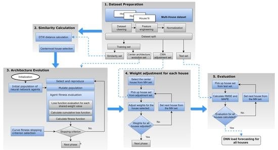
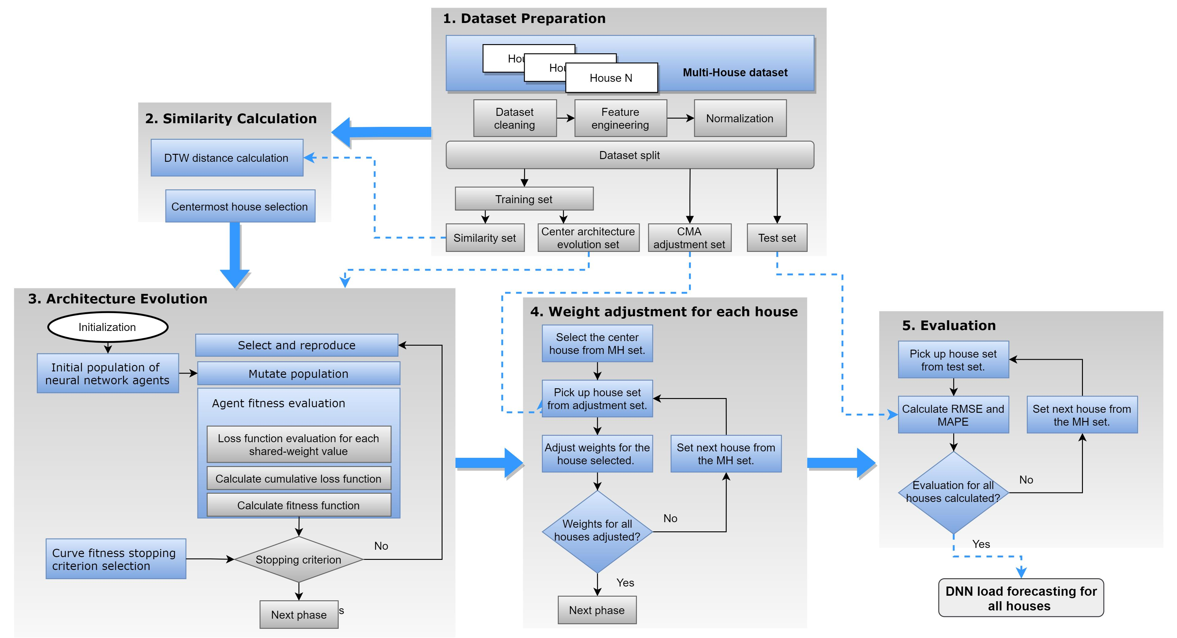
The centred architecture evolution search (SCAES) extends the DNN-CAE method [7], which is based on two main phases of evolution for a DNN. DNN-CAE first focuses the evolution efforts on the architecture development (phase 1). During DNN-CAE’s phase 1, each network agent’s fitness is measured using shared weight values. Then, in the following DNN-CAE phase, the weights are adjusted using the CMA-ES [40]. By using the DNN-CAE method, it is possible to separate weight dependence during the architecture evolution. Extending the DNN-CAE method, SCAES is implemented in five phases, as shown in Figure 1. Each phase performs processes that are required to develop a method that can create multiple forecasting models for a set of multiple houses. The framework presented in Figure 1 proceeds in the following order: in Phase 1, the data contained in the multihouse set is processed; Phase 2 searches for a house with a time series with the most similar pattern among the multihouse dataset; Phase 3 evolves the central architecture using the method presented in [7]; next, in Phase 4, the weight sets for each house are adjusted; and finally, Phase 5 evaluates each house’s performance. In the following subsections, each phase will be covered in detail.
3.1. Phase 1: Dataset Preparation
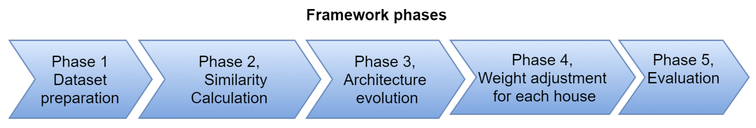
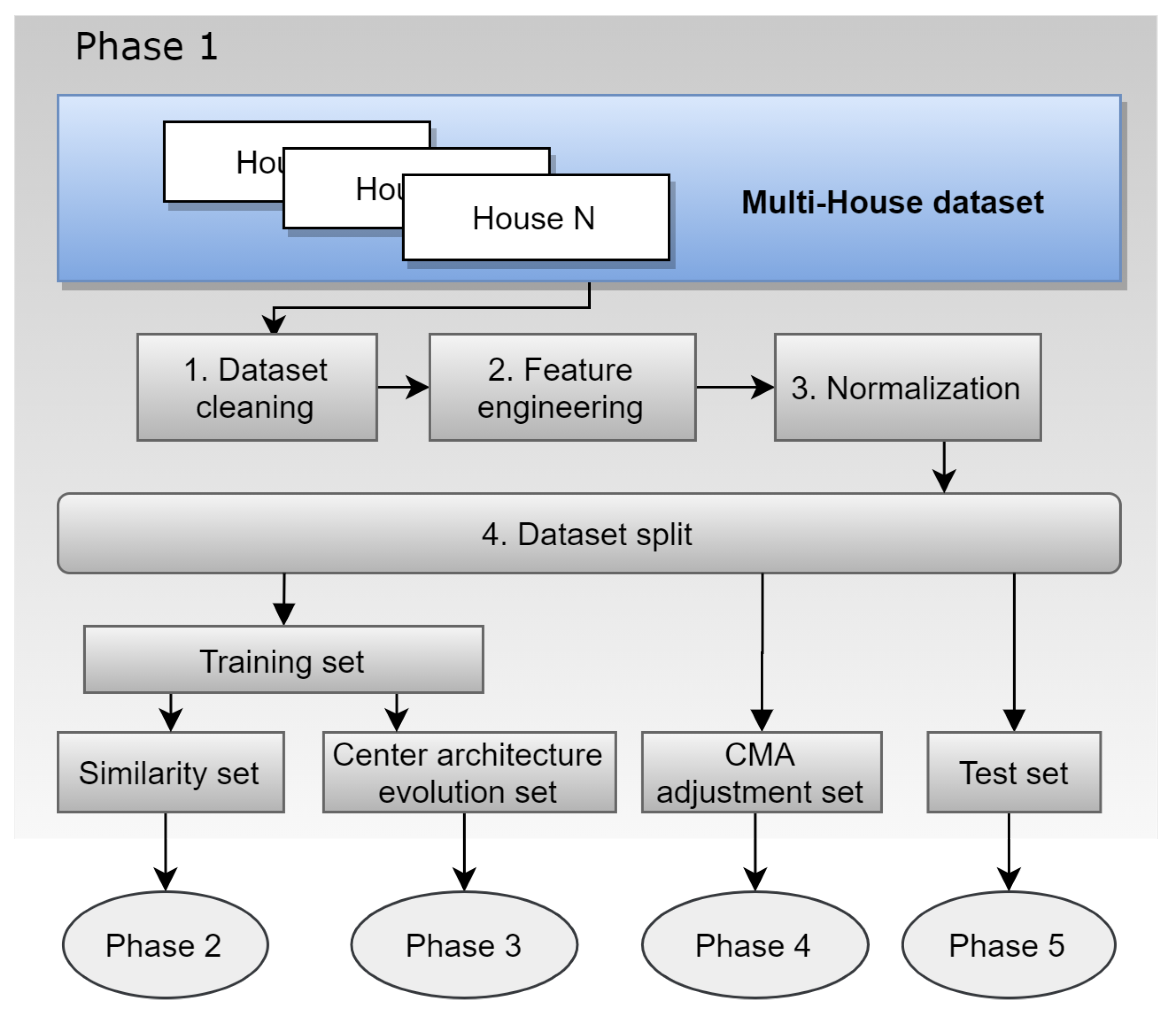
In this phase, the time series for all the houses are joined into one dataset, referred to hereafter as the multihouse (MH) dataset. Figure 2 shows the four steps performed during this phase: dataset cleaning, feature engineering, normalising, and splitting the MH dataset. The first three steps create consistent data among all the houses in the MH dataset. Splitting the MH dataset then creates the sets that will be used in the next phases.
3.1.1. Step 1: Multihouse Dataset Cleaning
In this step, all the NaN values are removed. Duplicates such as repeated date and time values for the same house are also removed. Anomalies such as nonsequential data and incorrect scale units are detected and removed. Finally, missing values are filled with the average of the previous and next cells for the same feature.
3.1.2. Step 2: Feature Engineering
In this step, the MH dataset features are augmented by adding new attributes such as temperature and weather conditions as categorical values. Weather conditions as categorical text data are transformed to categorical numerical data. Then, temperature and weather conditions columns are merged into the dataset according to the date and time index. New features are also added to the dataset, such as days of the week, is weekday, is weekend, is holiday, and seasons of the year. Finally, some cyclic features such as month, day, hour, and weekday are transformed through sine and cosine functions into cyclic values. Past values from the same set as new features are also added, such as previous target values from the last hour up to the last 48 h. Averages for the previous 24 and 48 h and values for the last week at the same time, for the last month, and for last year are calculated. In total, 128 features are augmented in this step. In summary, 15% of the augmented features are date- and time-related, 5% are related to weather conditions, 38% are related to the last 48 h of load consumption, 10% represent the same hour in past days for the last month, and the remaining portion is data with similar features as the last year.
3.1.3. Step 3: Normalization
In this step, the MH dataset is normalised by applying min-max normalisation, as shown in Equation (1). The maximum and minimum load consumption values for the MH dataset are stored. Later, in Phase 5, the minimum and maximum values are used to transform the forecasted values into the original scale.
3.1.4. Step 4: Dataset Split
In this step, the MH dataset is split into training, weight adjustment, and test sets in proportions of 60%-20%-20% respectively. The training set is used in two instances: first in Phase 2 to search for the time-series centremost house, and second in Phase 3 to evolve the architecture with shared weights for the centremost house. The weight adjustment set is used in Phase 4 to adjust the architecture weight for each house in the MH set. Finally, the test set is reserved for metrics evaluation in Phase 5.
3.2. Phase 2: Similarity Calculation
A similarity calculation is used in this phase to define which time series presents the closest similarity among all the houses in the MH set. The method presented by Tian et al. [33] to calculate similarity is reproduced in this phase. The similarity between two pairs of time series results is a numeric value calculated between each possible pair of houses in the MH set. Three methods were considered and analysed to calculate similarity: Euclidean distance (Equation (2)), Cosine (Equation (3)), and dynamic time warping:
where and are time series for a pair of houses in the MH set and N is the time series length.
Dynamic time warping (DTW) [41] is a generalisation of classical algorithms for comparing discrete sequences to sequences of continuous values. Given a pair of time series and , DTW aligns both series to minimise the difference between and . To achieve this, a matrix , is created, where each value is the distance between each element of and . To calculate the distance between these points, the Euclidean distance is used. A warping path, , is created with matrix D, where the path must start and finish in diagonally opposite corner cells of matrix D. The warping path is defined as , where . must satisfy the continuity constraint that restricts the allowable steps to adjacent cells. must also satisfy the monotonicity constraint that forces the points in the warping path to be monotonically spaced in time. Finally, the warping path that presents the minimum distance between the two series and is the optimal path for the DTW distance and is defined by:
Euclidean, Cosine, and DTW distance methods are used to determine the optimal method to select the centremost house among the MH similarity set. First, the similarity matrices , and are created using the Euclidean, Cosine and DTW distances, respectively. Secondly, the centremost houses , and for each method are selected. The selection is performed by calculating the house with the lower distance using Equations (5) and (6). Then, an architecture is evolved for each one of , and following the DNN-CAE method [7]. For each one of the evolved architectures, the weights are adjusted for each house in the MH similarity set. Finally, overall performance is calculated for Euclidean, Cosine and DTW methods.
Equation (5) calculates each house’s cumulative distance, and Equation (6) defines the centremost house with lower distance among the houses in the MH similarity set.
where is the total similarity for house k, n is the number of houses in the MH set, and is the contents of cell of , where M is lower triangular and .
Similarity Method Selection
Before moving to the next phases, it is essential to determine the similarity method to be used. Therefore, in this subsection, experiments and results are described to show which method (Euclidean, Cosine, or DTW) is the most suitable to calculate similarity among the residential time series set.
Because the time required to calculate the distance matrix for each distance method is extensive, the data length was reduced to the most recent year in the training set. A parallel computation method [42] was also applied to calculate the DTW distance reducing the computation time.
Experiments were performed to determine which of the distance methods (Euclidean, Cosine or DTW) is the most suitable method to select the centremost house among the residential time series set. The experiments and results described in this section are essential to select the distance method because the centremost house is required for further steps in the methodology. Three experiments for each architecture evolution for the houses , and were performed. Each architecture was evolved for 500 generations with a population of 100 agents. Generation and population values were selected to reduce the time required to complete the experiments in this phase. Table 1 shows the average results for the Euclidean, Cosine and DTW distance methods.
The DTW distance presents better overall performance among three methods chosen to calculate the similarity. Then, DTW distance is chosen to measure the similarity among residential load consumption patterns. Finally, the centremost house is used in Phase 3 for the neural architecture search.
3.3. Phase 3: Architecture Evolution
In this phase, the time series with the closest similarity from Phase 2 will be treated as a centremost house. From the MH training set, the centremost house training set is selected and becomes the only training set used for the architecture evolution. The architecture developed in this phase is the centred architecture that will be weight-adjusted for each house in Phase 4.
The work presented in this paper extends the DNN-CAE method [7] by evolving the central architecture for the centremost house time series from the MH training set. The main engine used to evolve the architecture in DNN-CAE is reproduced in this phase. DNN-CAE focuses on architecture evolution by reducing the importance of the weights. In summary, during the evolution phase, the architecture search avoids weight training and adjustment by sampling on different fitness measurements using shared weight values. Each network agent is evaluated over a set of shared weight values, and the cumulative loss function is recorded. Finally, the parents that will create the offspring are selected, and the process is repeated following evolution mechanics until the model with the best fitness is found.
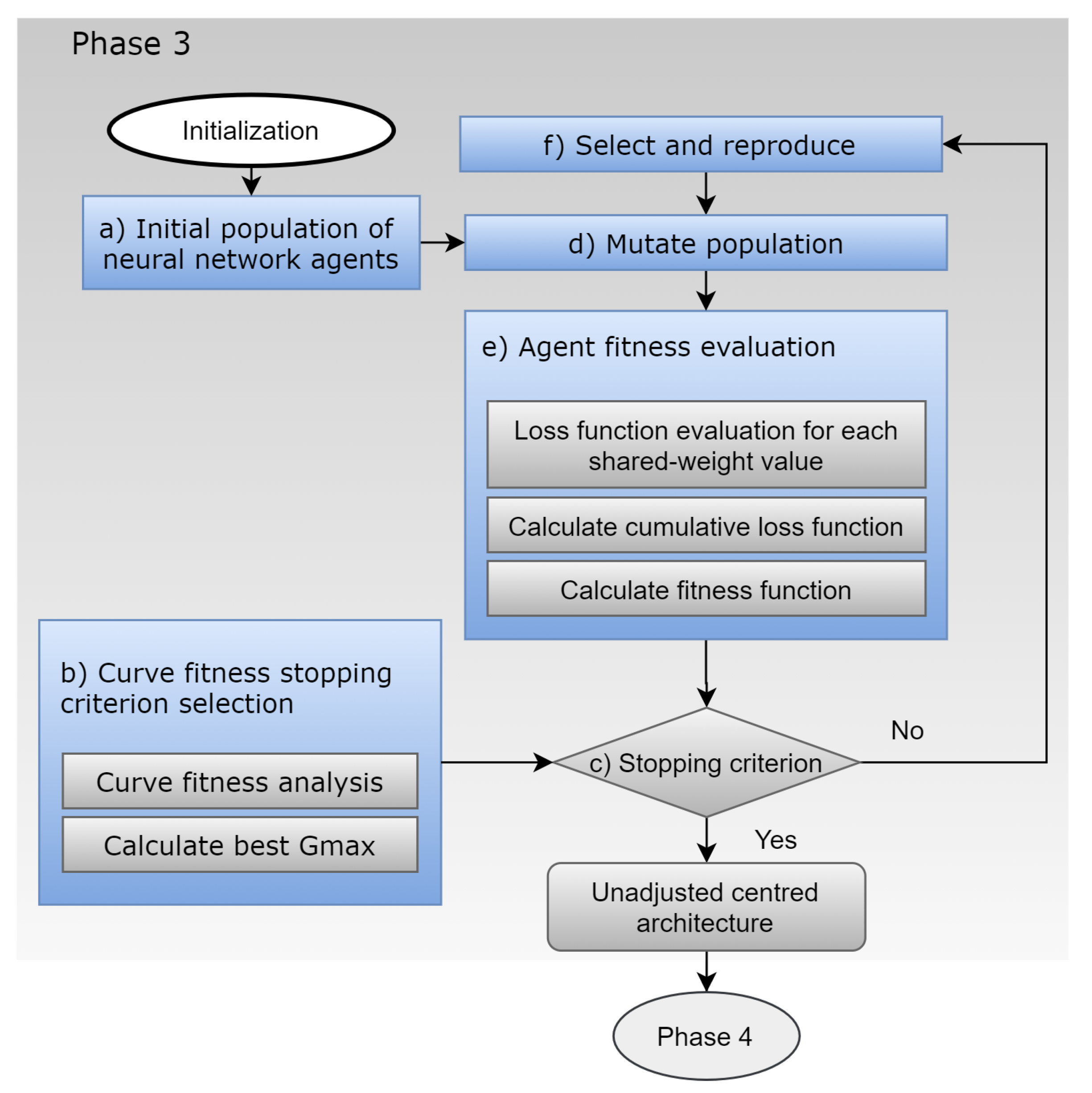
The steps performed in this phase reproduce the DNN-CAE steps [7] with one modification. As an update, the stopping criterion from DNN-CAE is enriched with an additional external step called the fitness curve stopping criterion, as shown in Figure 3. Table 2 shows the various parameters used in the architecture evolution. The rest of the steps can be summarised as follows:
- (a)
- First, all the parameters are initialised, and an initial population with a minimal network topology of size is created.
- (b)
- Fitness curve stopping criterion: In this step, the best maximum number of generations is defined by analysing curve fitness from several experiments. These experiments run outside the evolution cycle and before the main architecture evolution search. The objective of these experiments is to generalise fitness behaviour during architecture evolution. Consequently, the fitness evolution curve for the experiments is analysed. The maximum generation value that optimises the evolution search is then defined, and the parameter generation maximum is set to that value.
- (c)
- Following evolution mechanics, steps (d) to (f) are repeated until the maximum number of generations is achieved according to the stopping criterion step.
- (d)
- Mutation step: To avoid local optima, in each generation, mutation is performed over each neural network agent. Three mutations are implemented: (1) insert a node, (2) add a connection, and (3) change the activation function, and the probabilities that these mutations occur are set by the parameters , , and respectively. Parameter gives the list of the allowed activation functions.
- (e)
- Evaluate fitness step: In this block, three actions are performed in sequence as follows: first, for each agent, the neural agent loss function over a set of shared weights is evaluated; the neural agent’s cumulative loss function is then calculated; and finally, the neural networks agent’s fitness function is calculated.
- (f)
- Select and reproduce step: In this step, tournament selection is used to preserve the evolution process from stagnation through dominance by the best-fitness individual and to allow diversity during parent selection to create the next offspring.
3.4. Phase 4: Weight Adjustment for Each House
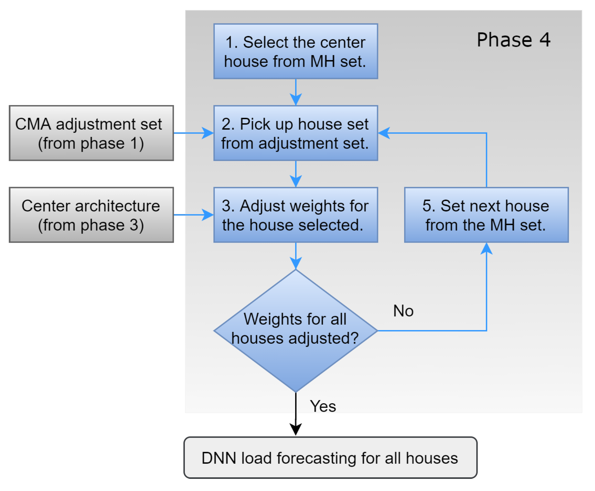
In this phase, the weights are adjusted for each house defined in the MH weight adjustment set. The centred architecture evolved in Phase 3 is used as the architecture for each house model. The centred architecture starts with a shared weight set, and using an evolutionary technique called CMA-ES [40], weights are adjusted individually. The sequence performed to adjust the weights for each house is shown in Figure 4.
The covariance matrix adaptation evolution strategy (CMA-ES) [40] is a type of black-box optimisation technique based on EA for nonlinear and nonconvex problems. CMA-ES is considered state of the art in evolutionary computation and is one of the standard tools for continuous optimisation problems. This approach creates a covariance matrix describing the correlations between decision variables. Then, through evolution mechanics, the matrix likelihood is maximised, generating successful solutions. The CMA-ES state variables, for a space of dimension N, are given by the distribution mean , the step size , and the covariance matrix . CMA-ES is an iterative algorithm that, in each of its iterations, samples candidate solutions from a multivariate normal distribution, evaluates them, and then adjusts the sampling distribution used for the next iteration.
The CMA-ES technique is used to evolve the centred architecture weights and tune the DNN model for each house. This step uses what can be considered a baseline version, featuring nonelitist selection. All tuning constants are set to their default values, as stipulated by Hansen [43]. As shown in Figure 4, the centremost house is first selected, and then the adjustment set that belongs to that house is extracted. Next, the architecture weights are adjusted using the CMA-ES technique. The interactive process then moves forward to the next house in the MH set until all the house models have had their weights adjusted.
The approach presented in this phase becomes a transfer learning method, where the process learned for one model can be transferred to another model with similar characteristics, thus saving computing time. Using a centred architecture saves the time needed to build a separate model for each house because the centre architecture has been evolved to retain the general patterns for residential load consumption. Then, by adjusting the weights, which takes 80% less time than evolving a new architecture, the model as tuned can forecast each house’s load consumption with good accuracy.
3.5. Phase 5: Evaluation
In this phase, each house model with adjusted weights and centred architecture is evaluated. For this purpose, the test set corresponding to each house is retrieved from the MH test set from Phase 1. The metrics the root mean square error (RMSE) (Equation (7)) and the mean absolute percentage error (MAPE) (Equation (8)) are calculated to measure model performance over the selected house test set. RMSE and MAPE were selected because of their frequent use in energy forecasting studies [12].
where denotes the predicted consumption, denotes the actual electricity consumption of the household and n is the number of observations.
Other metrics such as mean absolute error (MSE) and mean square error (MSE) were also calculated in the experiments, but they are not shown here because they exhibited the same patterns as RMSE and MAPE.
4. Sensitivity Analysis
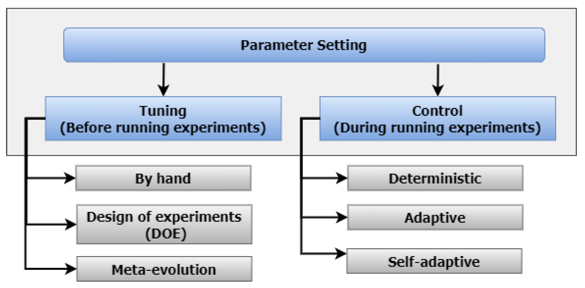
Sensitivity analysis is a technique used to identify how the different values of a set of parameters influence the uncertainty of a model’s output under certain specific conditions. In general, sensitivity analysis is used in various fields such as biology, economics, and engineering. In the field of EA modelling, this technique can answer questions such as which factors cause the most and the least uncertainty in model accuracy [36]. Sensitivity analysis is advantageous when used together with design of experiments (DOE) to set model parameters. This method enables the designer to obtain a broad view of the factors that most strongly influence model performance. In contrast, the less influential parameters can be set to arbitrary values, saving time during evolutionary mechanics. According to Kramer [44], EA parameter setting is divided into two categories: tuned parameters, for setting parameters before the algorithm runs; and control parameters, to control algorithm performance while the experiment runs. Figure 5 shows these parameter setting categories.
Figure 5 shows that the parameters tuning are divided into three components: by hand, DOE, and metaevolution. Tuning by hand is probably one of the most used approaches to parameter setting, but it is highly dependent on designer expertise, and the results may not always be optimal. Tuning using DOE is another technique commonly used in EAs, with good results. Well-chosen DOEs maximise the information obtained for a given amount of experimental effort. Metaevolution uses a two-level evolutionary optimisation process to automatically search for the parameters in an outer loop while an inner loop searches for the model optimisation. The disadvantage of using metaevolution is the massive computing power required to evaluate the optimal parameters. Therefore, this study used DOE as the tuning method to study the influential parameters for SCAES. The objective of using sensitivity analysis in SCAES was to reduce the EA parameter search space.
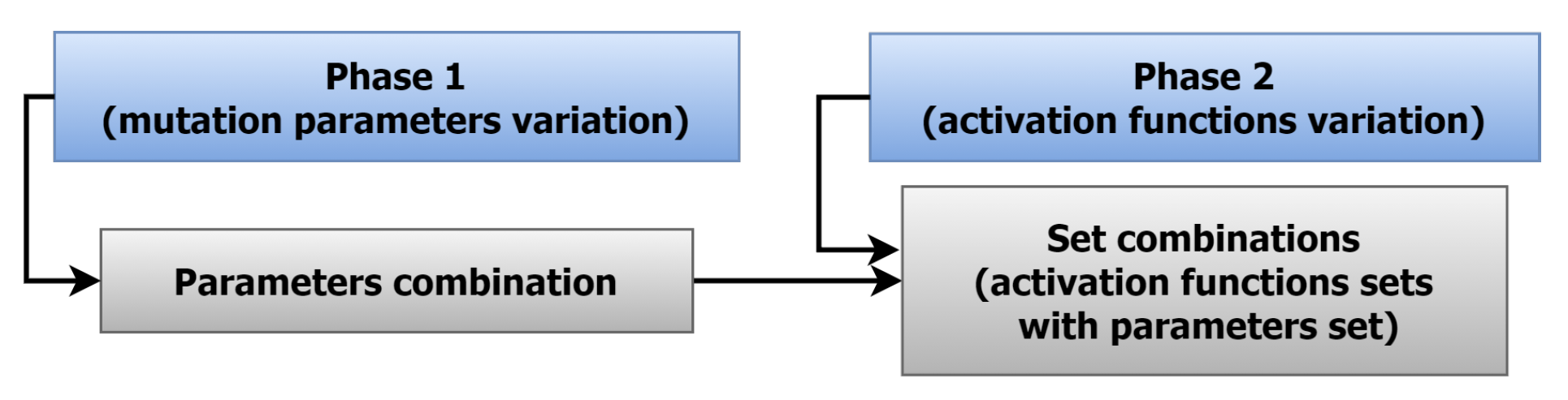
Among the set of all possible parameters in Table 2 to be analysed for SCAES, four parameters played an essential role in the neural architecture search: the probability of adding a connection (), the probability of adding a node (), the probability of changing an activation function (), and finally the set of activation functions (). Two phases were performed to analyse the model’s sensitivity to the four parameters, as shown in Figure 6. In the first phase, the three mutation parameters , , and were analysed. Phase 1 evaluated the effect of each parameter variation by combining variations on the three parameters (parameters combination) during the experiments. Finally, in the second phase, the activation function was evaluated after selecting the best combination of mutation parameters from phase 1.
4.1. Phase 1: Sensitivity Analysis for Mutation Parameters
In this phase, the single-value mutation parameters , , and are evaluated. Each parameter varies over the range [0, 1]. A value of 0 means that no mutation is allowed, and a value of 1 means that mutation is performed in all the mutation steps in the evolution mechanics. Mutations are constrained to the range [0.25–0.75] to create relevant results. When a mutation in a network agent is activated by , a sequence of actions occurs. First, a node is selected randomly. Then the node changes its activation function to another one chosen randomly. The set of possible activation functions consists of , , , , , , , and . The available activation functions are set to 9, enabling the use of any activation function described. In this phase, the architecture is evolved first, and then the architecture weights are adjusted using the CMA-ES technique. The model’s accuracy with the parameters under analysis is then evaluated. As shown in Figure 6, a sensitivity analysis for the parameter combination is performed in this phase.
In this phase, the variation of the combined parameters was investigated to evaluate the interaction between parameters. For this effect, the method presented by Pinel et al. [45] was reproduced. The method random balance designs Fourier amplitude sensitivity test (RBD-FAST) [46] was used to reduce the large requirement of samplings presented in [45]. This method computes the first-order effects and interactions of the three parameters , , and . In addition, Latin hypercube sampling [47] was used to generate the sampling of the parameters combination.
4.2. Phase 2: Sensitivity Analysis for Activation Functions
In this phase, the uncertainty generated by the set of activation functions was analysed. Following the analysis performed in [7], three sets of activation functions were considered. The sets were called , containing three of the most used activation functions (inverse, absolute, and ReLu); , containing sigmoid, hyperbolic tangent, inverse, absolute, and ReLu; and finally, , with all the activation functions available. The process performed in this phase required the set of combined factors from Phase1.
5. Results
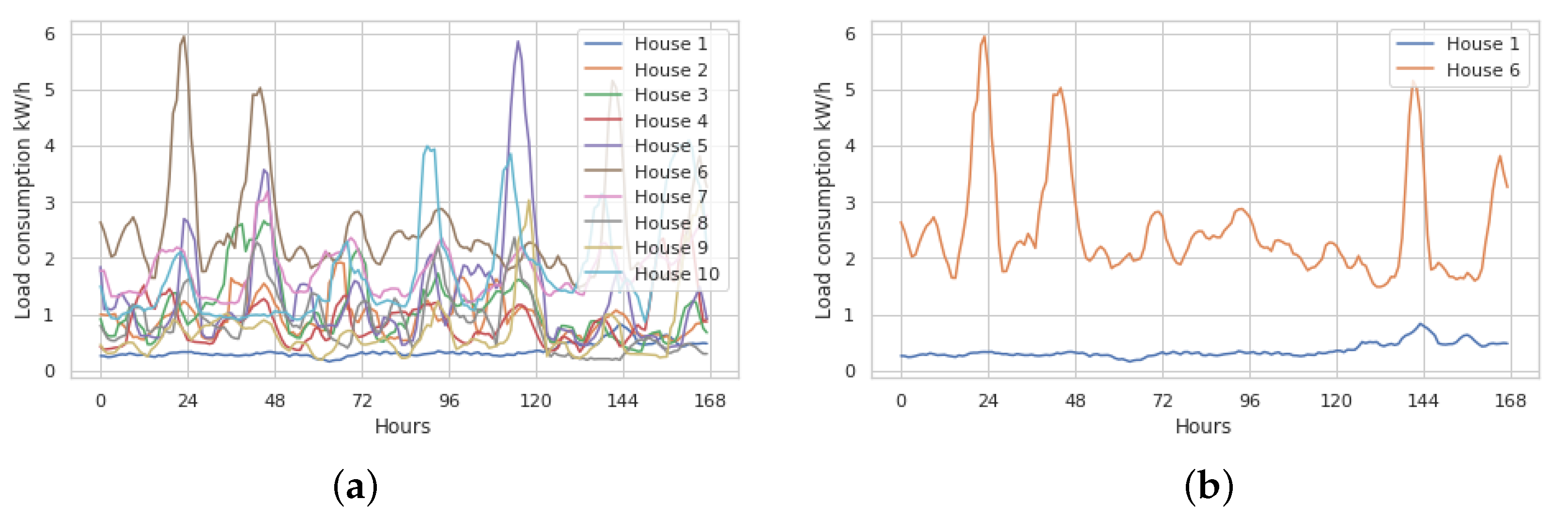
Electricity consumption patterns for a house are complex and nonlinear. Hence, forecasting the next hour’s consumption for a house is challenging. This task becomes even more complex if a method must forecast multiple houses. Each house presented unique characteristics depending on the hour of the day, the day of the week, and in some cases, the season of the year. The records of ten houses for one week in 2016 are shown in Figure 7a. Clearly, although a subset of the houses exhibited similar behaviour, houses such as 1 and 6 presented markedly different behaviours, as shown in Figure 7b.
SCAES was used for short-term load forecasting for a set of multiple houses in a neighbourhood. The residential dataset was provided by the London Hydro utility company. The multihouse (MH) set contained readings from ten smart meters from a neighbourhood where houses presented similar characteristics, e.g., square footage, number of bedrooms, household appliances or AC. The dataset registered hourly records from 1 January 2014, to 31 December 2016. Historical hourly weather and temperature data were obtained from the official Canadian Government Web site [48]. SCAES forecasted the next hour’s consumption for each house in the MH set to apply a centralised architecture and adjust the weights of a transfer learning model. All the models and experiments were run on a Linux server with 24 Intel(R) Xeon(R) E5-2630 v2 processors, and the model was implemented in Python language, version 3.7. The package developed by Herman and Usher [49] was used to ran sensitivity analysis experiments in Python environment, and package [42] was used to calculate DTW distances faster.
The following subsections describe the investigation of different experimental cases. Each case was explored using a suite of experiments to analyse model behaviour and show SCAES functionality. The idea behind the sequence of experimental cases was to prove the validity of SCAES. Simultaneously, this sequence provided NAS enthusiasts with a guide to set up NAS models using evolutionary algorithms (EAs). The experimental cases in the following subsections were divided into two categories: those that analysed model behaviour (sensitivity analysis) and those that defined model performance (parameter selection analysis).
In the first category, Case 1 was investigated to calculate the time series similarity among the houses. The DTW distances were calculated, and the centremost and farthest houses were defined from the MH set. This step was essential to continue with the sequence of experiments because the centremost and farthest houses were required in the design of experiments (DOE) for the following subsections. Next, in Case 2, the sensitivity of the evolutionary parameters was analysed. Sensitivity analysis is useful when applying EAs to NAS because it reveals each parameter’s influence on architecture evolution and consequently on architecture performance. Then, in Case 3, parameter values were selected that optimised model performance.
The experiments performed in the first category helped to understand and improve SCAES performance. By following the sequence of experiment cases, at the end of Case 3, the set of parameters that would be used in the second category of experiments was also defined.
The second category investigated model performance. Case 4 experiments were performed to show how SCAES forecasts load consumption for each house in the MH set. Finally, Case 5 implemented a benchmark comparison between SCAES and other state-of-the-art models.
5.1. Case 1: Similarity Calculation
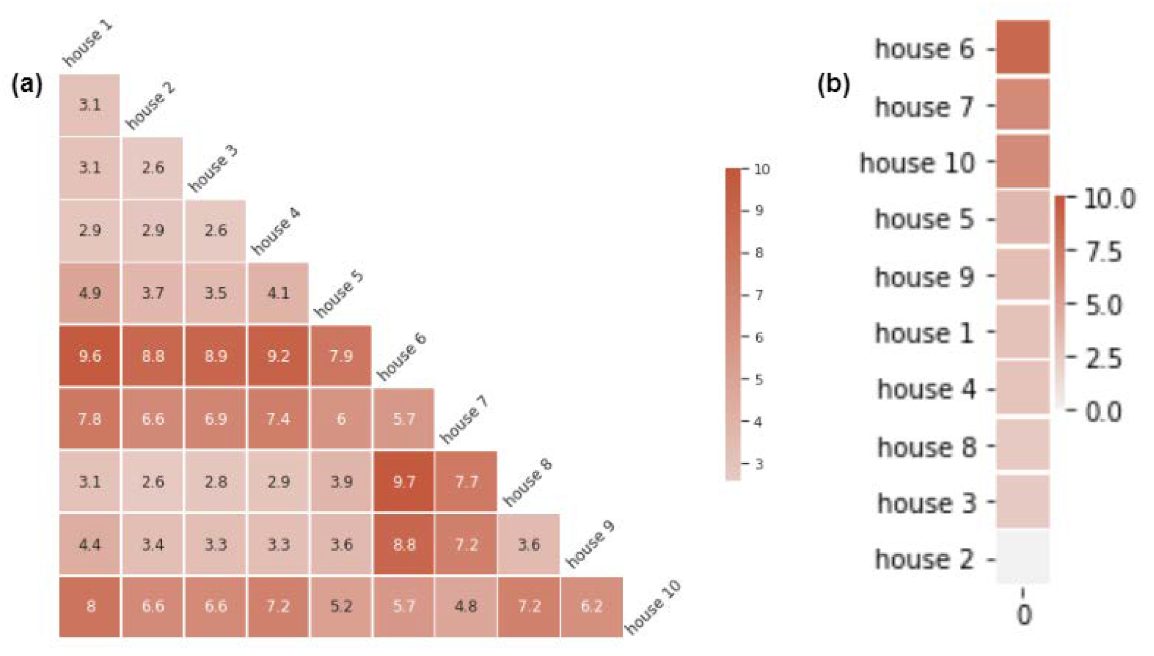
This suite of experiments formed part of the model behaviour analysis category. These experiments were essential because they defined the centremost and farthest houses from the MH set. Case 1 analysed the similarity distances among the time series in the MH set by calculating the DTW distance. A similarity matrix M was created using the DTW distances, where M was a lower triangular matrix with the diagonal set to zero. Figure 8a shows the similarity matrix. The similarity was calculated using the last year of data from the MH training set. Equation (5) was used to calculate the total similarity among the houses.
For example, for house 6, the total similarity was calculated as follows:
and referring to the values in Figure 8a, .
In this way, each house’s total similarity was calculated, and the houses with the lowest and highest values became the centremost and farthest houses respectively. When the houses’ total similarity was calculated, house 2 became the centremost house, with , and the farthest house was house 6, with .
5.2. Case 2: Sensitivity Analysis
This suite of experiments belonged to the model behaviour analysis category. The performance and uncertainty of the model were analysed using sensitivity analysis methods. The mutation parameters used for architecture evolution were the probability of adding a connection, , the probability of adding a node, , and the probability of changing an activation function, . , , and were analysed in DOE 1. Each parameter , , and varies over the range [0, 1]. A value of 0 means that no mutation is allowed, and a value of 1 means that mutation is performed in all the mutation steps in the evolution mechanics. Mutations are constrained to the range [0.25–0.75] to create relevant results.
The selection of the activation functions in the activation function set, referred to hereafter as (), was analysed in DOE 2. When a mutation in a network agent is activated by , a sequence of actions occurs. First, a node is selected randomly. Then the node changes its activation function to another chosen randomly. The set of possible activation functions consisted of , , , , , , , and . In DOE 2, three sets of possible activation functions were chosen for the sensitivity analysis. The first set, , had only , , and activation functions; the second set, , had the most used activation functions available (, , , , and ). Finally, the third set, , had all the activation functions available.
The sensitivity analysis was performed in a sequence of two DOEs. In DOE 1, the sensitivity analysis was conducted with combinations of the factors , , and . In this DOE, the random balance designs Fourier amplitude sensitivity test (RBD-FAST) [46] was used to compute each factor’s influence. RBD-FAST was selected among other sensitivity analysis methods, such as Morris [50] and Fourier amplitude sensitive test [51], because RBD-FAST was the updated method, and the computing time was reduced in comparison with the other mentioned methods. Finally, in DOE 2, the factor was analysed, along with the resulting interaction with . The three DOEs were expected to characterise the model’s behaviour as the variation of its principal parameters , , and and the selection of .
Sensitivity analysis makes it possible to understand the influence of each parameter in the outcome of SCAES. Because architecture evolution is a random process, five repetitions were performed for each DOE to ensure that the sensitivity analysis was correct. The architectures evolved in this subsection were implemented with a population of 120 neural network agents for 250 generations. For each architecture evolved, the weights for the centremost and farthest houses were adjusted.
5.2.1. Design of Experiments 1: Combined Factor Analysis
In this DOE, the evolution process was run with combinations of the factors , , and . was chosen as as explained in Case 2 Senstivity Analysis. The technique called Latin hypercube sampling [47] was used to generate the sampling combinations of factors. According to Tarantola et al. [46], Latin hypercube sampling is the best sampling technique associated with RBD-FAST. The sampling scheme was set to 50 samples with three factors, and five repetitions were performed for each combination. The variation allowed for each factor was set as the range [0.25–0.75] (as explained in Case 2, sensitivity analysis). In total, 500 experiments were performed in DOE 1. Table 3 shows a summary of the settings for DOE 1.
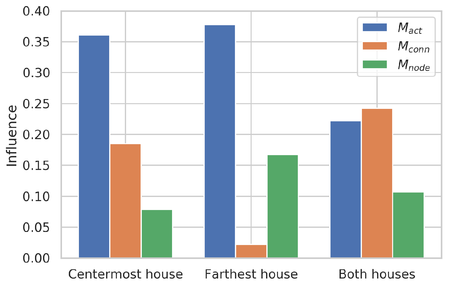
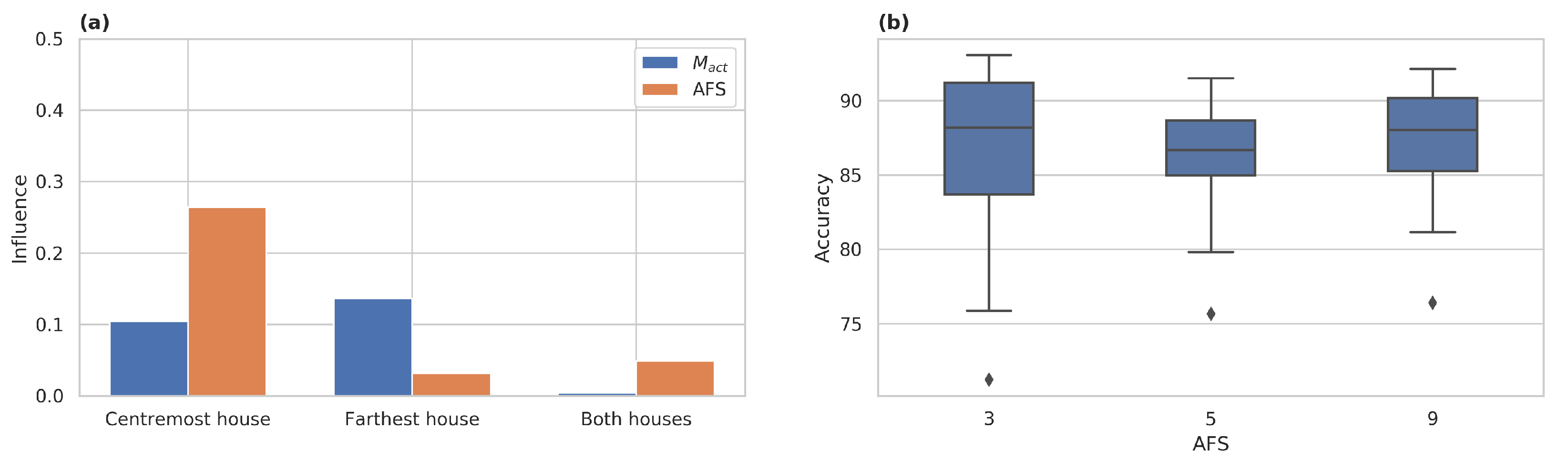
RBD-FAST was used to compute each factor’s influence on model performance. Three RBD-FAST calculations were performed. For the centremost and farthest houses, independent RBD-FAST calculations were performed, and for both houses’ general outcome, a separate RBD-FAST was also calculated. Figure 10 shows how each factor influenced model performance for each house and for both houses. The factor continued to play an essential role in model performance, accompanied by the factor . As shown in Figure 10, had a higher value when it was analysed for each house individually, probably because the variance was calculated explicitly with the model performance. However, had reduced influence in the case of both house generalisation.
5.2.2. Design of Experiments 2: Analysis of Sets of Activation Functions
In this DOE, a suite of experiments was performed to analyse the architecture evolution behaviour with a restriction on the available activation functions. The available sets of activation functions were chosen as , , and , which were described in Case 2 sensitivity analysis. As seen in DOE 1, played an essential role in the model’s influence and was related to the activation function sets. Three variations were allowed for , whereas were fixed to 0.5. Three repetitions were performed for each combination. In total, 54 experiments were performed in this DOE. Table 4 shows a summary of the settings for DOE 2.
Figure 11a shows the results for the three RBD-FAST calculations. As shown in Figure 11a, the played an essential role in model performance. Figure 11a shows that the centremost house was influenced explicitly by the factor. For the farthest house, the factor had a greater influence on the model, probably because of the differences in the two houses’ patterns. In contrast, the had more influence in the case of both houses. Figure 11b presents the general model performance over the factors analysed. The figure shows that presented consistent behaviour, but that , despite its higher variance, could lead to better accuracy.
5.3. Case 3: Parameter Selection Analysis
This suite of experiments also formed part of the model behaviour analysis category. The work described in this subsection was essential for good performance of SCAES in the following category of experiments because it analysed the set of parameters that optimised SCAES. Moreover, as seen in the previous subsection, and the had the greatest influence over the model outcome. Consequently, this subsection will describe the determination of the best set of values for and the . Two DOEs were designed to optimise SCAES performance and are described in this subsection. The first DOE analysed combinations of the factors , , and with the chosen as . The purpose of this DOE was to find the set of best combinations for , , and , keeping in mind to select the best sets for . Once the combinations were defined, the next DOE, where the varied, was executed. In DOE 1, the combination of and the was analysed to define the parameters that optimised model performance. Because architecture evolution is a random process, to ensure the validity of the DOE 3 and DOE 4 results, five and three repetitions were performed respectively. The architectures were evolved with a population of 120 neural network agents for 250 generations. For each architecture evolved, the weights for the centremost and farthest houses were adjusted.
5.3.1. Design of Experiments 3: Parameter Combinations for Parameter Selection
In this DOE, the evolution process was run with a combination of factors , , and . Three variations were allowed for each factor, where , , and the was chosen as . In total, 270 experiments were performed in DOE 3. Table 5 shows a summary of the settings for DOE 3.
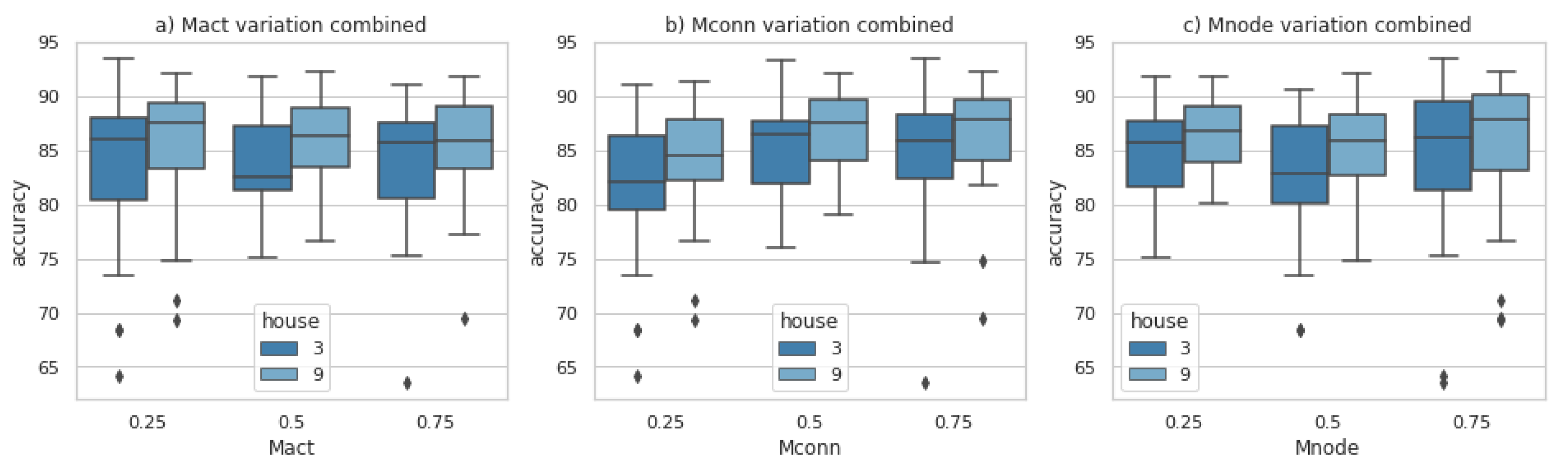
Figure 12 shows the architecture performance when varying each factor. Each plot presents the results for the centremost and the farthest house. As shown in Figure 12a, was accurate for both houses at a value of 0.75, and a similar situation occurred for at a value of 0.25, as shown in Figure 12c. However, in Figure 12b, presented diversity in the results between the two houses.
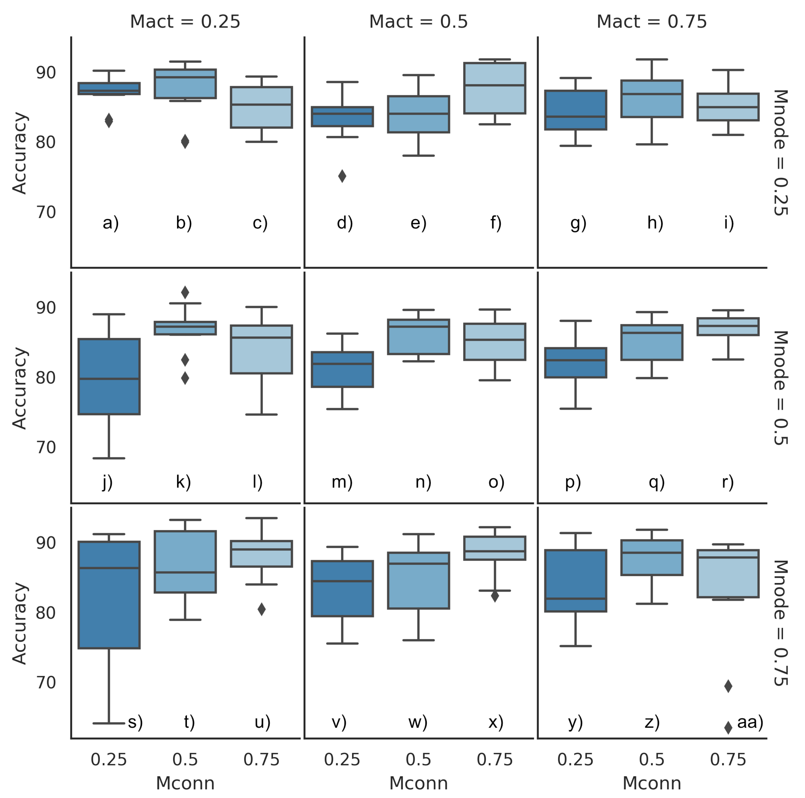
Figure 13 shows a box plot matrix with the results for DOE 3. The box plot matrix helps to visualise the architecture performance with factor variation. Each boxplot was the result of five experiments with adjustments for h2 and h6. In general, was precise for a value of 0.25, with an accuracy higher than 80%. If model performance is tracked with , it can be stated that performed well for a value of 0.5.
This DOE was intended to find the best set of parameters for . As shown in Figure 13, the box plot (b) (column ) gave the highest accuracy; the box plot (x) (column ) had the best performance, and for the box plot (r) (column ) was the best option. Hence, the combinations of , , and that optimised model performance were defined by cases (b) and (r).
5.3.2. Design of Experiments 4: Activation Function Combination for Parameter Selection
In this DOE, the sets of combinations (b), (x), and (r) from DOE 3 were selected to be combined with the . The three cases selected from DOE 3 were the optimal cases for . Each case was combined with each one of the . In this DOE a third house randomly selected (h9) is analysed for better generalisation. Three repetitions were performed for each experiment with adjusted houses [h2,h6,h9]. In total, 54 experiments were performed in DOE 4. Table 6 shows a summary of settings for DOE 4.
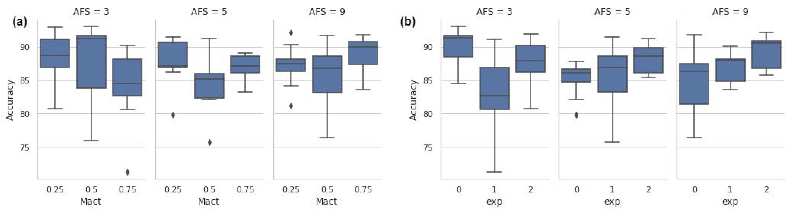
Figure 14 shows the results for DOE 4. The model performance for each activation set is presented in two scenarios. In the first scenario, Figure 14a shows how the model behaved as varied. The second scenario shows the overall performance of each experiment for each of . Even if the results for set showed better accuracy for experiments 1 and 3, experiment 2 had lower accuracy, showing that the results of were highly variable. On the other hand, performed consistently for both scenarios.
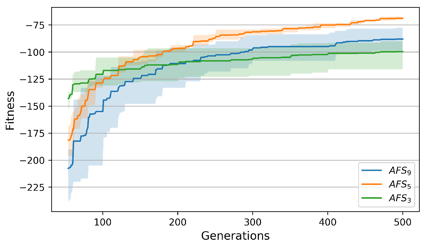
Figure 15 shows the curve fitness for the three during architecture evolution. Set achieved a steady state after 100 generations, but it got stuck in that state. Set took a longer time to stabilise, doing so after approximately 300 generations. In contrast, set stabilised after outperforming the other two sets after 150 generations. Consequently, the best set of parameters to evolve the architecture was given by with , , .
5.4. Case 4: Load Forecasting for Multihouse Set
This suite of experiments was the first set of experiments in the model performance category. This case aimed to demonstrate SCAES functionality for load consumption forecasting for each house in the MH set. Phases 3, 4 and 5 from the methodology section were implemented as described in this subsection to create forecasting models. Each forecasting model resulted from adjusting the centre architecture weights to a specific house in the MH set. The centre architecture was evolved with the set of parameters selected from DOE 4. Two steps were performed in the work discussed in this subsection: first, a curve analysis to define the stopping criterion maximum generation , and then the creation of the models for load forecasting.
5.4.1. Fitness Curve Stopping Criterion Analysis
In this step, the architecture fitness performance over the generations was analysed. As explained in the Phase 3 of the methodology, this analysis was performed outside the evolution cycle and previously ran the main architecture evolution search. The objective of these experiments was to generalise fitness behaviour during architecture evolution by selecting the best generation at which to stop the evolution process.
Three repetitions were performed for the architecture evolution. Every 20 generations, the architecture was recorded, and the process continued until 500 generations were reached. Similar as in DOE 4, a third house (h9) is selected for better generalisation. Finally, the average, minimum and maximum values were calculated for houses h2, h6 and h9. In total, 225 experiments were performed in this step.
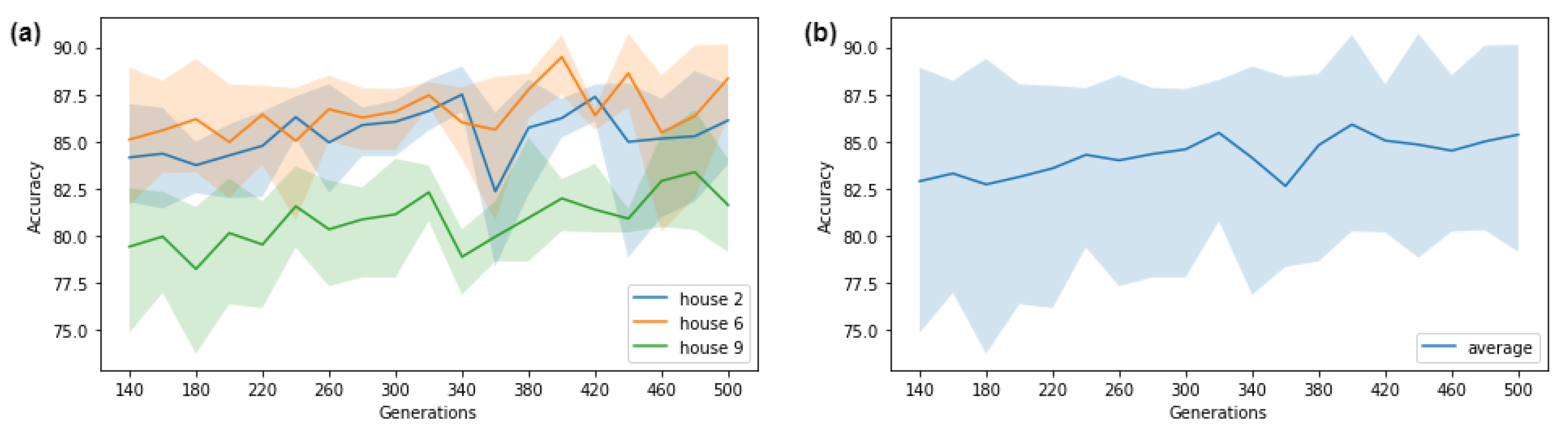
Figure 16 shows the model performance over two scenarios. The first scenario, Figure 16a, shows the architecture performance with adjusted weights for houses h2, h6 and h9. The second scenario, Figure 16b, shows the average band of operation for the architecture evolution. As shown in Figure 16a, the best accuracy for the three houses occurred at generations 320 and 400. was set to 320 because this value shortened evolution time consequently reducing network complexity.
5.4.2. Load Forecasting Results
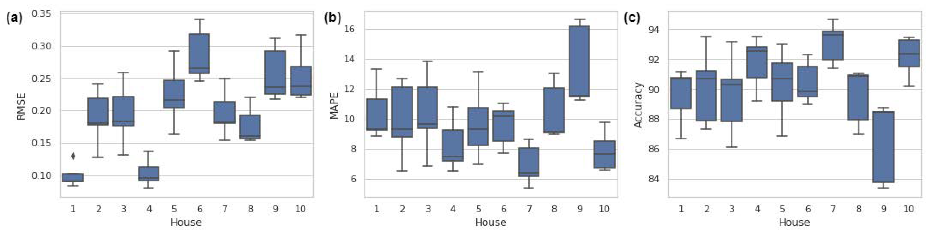
In this step, the centre architecture was evolved. Then the architecture weights were adjusted using the CMA-ES technique for each house in the CMA adjustment set from the Phase 1 in the Methodology. Ten repetitions were performed for the architecture evolution and their respective adjusted weights. Table 7 shows the parameters used for the architecture evolution. Figure 17 shows the ten houses’ performance for load forecasting after the architecture weights were adjusted. The RMSE and MAPE metrics were calculated using the MH test set. Accuracy was expressed in terms of MAPE. The lower the values for RMSE and MAPE, the lower was the error, and hence the better the performance was. In addition, the higher the accuracy, the better was the model performance.
Figure 17 shows that the model performance results were diverse. For most houses (except house nine), the proposed approach achieved good performance, with errors in the range of 6% to 14%, as shown in Figure 17b. For house nine, the error was in the range from 11% to 17%. In general, the error of the proposed approach was less than 17%.
5.5. Case 5: Benchmark Comparison
This suite of experiments was the last case in the model performance category. Case 5 implemented a benchmark comparison between SCAES and other state-of-the-art models to prove the proposed model’s functionality. SCAES forecasting results were compared with LSTM load forecasting models and traditional feed-forward ANN. For comparison purposes, the benchmark presented by Kong et al. [12] was reproduced. The methods selected for the comparison were feed-forward neural network (FFNN), vanilla LSTM, LSTM augmented features and LSTM one-shot (LSTMOS). FFNN is a conventional backpropagation neural network model. Vanilla LSTM is the simplest method. However, the LSTM features model was used to augment its inputs with additional features such as time, weekdays and holidays. LSTMOS [12] is state of the art in residential load forecasting. Table 8 presents the parameters used to configure the LSTM models. LSTMOS was trained with different backward time steps. To follow the convention used in [12], -T represents backward hour steps and -D represents backward day steps. Finally, the average, minimum and maximum were calculated as metrics for the entire MH set.
Table 9 presents the results for the three LSTM models and SCAES. The total average for RMSE, MAPE and accuracy were calculated for each method. Additionally, Table 9 shows the individual average results for the best house, the centremost and farthest houses.
In terms of LSTM models for multiple houses load forecasting, the best LSTM model for the average of house results was the LSTMOS/6 with 88.06% accuracy. The house with the lower average error for LSTM is h2 with 8.58%. Clearly, Feed-forward NN models presented the worst performance among all the benchmark comparison set, with errors in the range of 18.8% to 23.7%. Interestingly for LSTMOS/6 both centremost and farthest houses present similar performance. Table 9 shows that SCAES performs better than the presented techniques with 3.17% accuracy. Moreover, the method proposed presents the best house performance with the lower error of 6.56%.
6. Discussion
This paper shows that the evolutionary NAS approach to load forecasting for multiple houses is feasible. The results are comparable to state-of-the-art LSTM models, and it is attainable for real-world applications. Once the architecture has been evolved from the centremost house, it can be transferred to other houses in the set. The time required to adjust the weights in all the cases is four times lower than evolving a new architecture for each house from scratch. It is important to note that the approach is still under development. The method requires a couple of hours to evolve the centre architecture over a multiprocessor server, and throughout its evolution, thousands of neural network agents are created. Therefore, the results are limited by the available computational power.
The sensitivity analysis has been useful in defining each parameter’s influence over the model performance. The results are promising because they brought the first exploration for parameter selection, which incurs the model performance over 90%. The method presented in this work could be useful for EAs enthusiasts as a guide for parameter selection.
7. Conclusions
This paper proposes a similarity centred architecture evolution search (SCAES) to enable residential deep neural network-based forecasting models for a multihouse (MH) set. First, the model evolves a centred architecture based on the MH set’s centremost time series house. Later, the architecture weights are adjusted for the other houses in the set. The evolution starts with simple neural architecture agents and grows in complexity as the model evolves. During evolution, the mutation is performed for each agent. The mutation parameters were selected from the sensitivity and parameter selection analysis. The centred architecture weights are then adjusted for each house in the MH set, creating a set of forecasting models. In addition, after running two experiment cases for the model performance, SCAES showed an accuracy of 91.23% on average for the MH set. Future work will further explore the impact of new techniques to reduce the architecture evolution time. For instance, it may be possible to seed the population with various state-of-the-art architectures and modules instead of rediscovering them during evolution. Other methods such as partially evolved architectures can be explored to reduce the computational power required. Interestingly, evolution can be guided with goals other than simple accuracy, including training time and execution time, which open new development opportunities for SCAES.
Author Contributions
Conceptualization, S.G.-R.; methodology, S.G.-R., and M.A.M.C.; investigation, S.G.-R.; data curation, S.G.-R.; writing—original draft preparation, S.G.-R.; writing—review and editing, S.G.-R., and M.A.M.C.; supervision, M.A.M.C.; funding acquisition, M.A.M.C.; data provision as industrial partner, S.M. All authors have read and agreed to the published version of the manuscript.
Funding
This research was funded by Natural Sciences and Engineering Research Council of Canada: 530743-2018-CRDPJ, SENESCYT scholarship from Ecuador: Convocatoria abierta 2016.
Conflicts of Interest
The authors declare no conflict of interest.
References
- Morstyn, T.; Farrell, N.; Darby, S.J.; McCulloch, M.D. Using peer-to-peer energy-trading platforms to incentivize prosumers to form federated power plants. Nat. Energy 2018, 3, 94–101. [Google Scholar] [CrossRef]
- Eid, C.; Codani, P.; Perez, Y.; Reneses, J.; Hakvoort, R. Managing electric flexibility from Distributed Energy Resources: A review of incentives for market design. Renew. Sustain. Energy Rev. 2016, 64, 237–247. [Google Scholar] [CrossRef]
- International Energy Agency. World Electricity per Capita. Available online: https://www.iea.org (accessed on 30 August 2020).
- Haider, H.T.; See, O.H.; Elmenreich, W. A review of residential demand response of smart grid. Renew. Sustain. Energy Rev. 2016, 59, 166–178. [Google Scholar] [CrossRef]
- Zoph, B.; Le, Q.V. Neural architecture search with reinforcement learning. In Proceedings of the 5th International Conference on Learning Representations, ICLR 2017—Conference Track Proceedings, Toulon, France, 24–26 April 2017. [Google Scholar]
- Lu, Z.; Deb, K.; Goodman, E.; Banzhaf, W.; Boddeti, V.N. NSGANetV2: Evolutionary Multi-Objective Surrogate-Assisted Neural Architecture Search; Vedaldi, A., Bischof, H., Brox, T., Frahm, J.M., Eds.; Springer International Publishing: Berlin/Heidelberg, Germany, 2020; pp. 35–51. [Google Scholar] [CrossRef]
- Gomez-Rosero, S.; Capretz, M.; Mir, S. Deep neural network for load forecasting centred on architecture evolution. In Proceedings of the 2020 19th IEEE International Conference on Machine Learning and Applications (ICMLA), Miami, FL, USA, 14–17 December 2020; pp. 122–129. [Google Scholar] [CrossRef]
- Klyuchnikov, N.; Trofimov, I.; Artemova, E.; Salnikov, M.; Fedorov, M.; Burnaev, E. NAS-Bench-NLP: Neural Architecture Search Benchmark for Natural Language Processing. arXiv 2020, arXiv:2006.07116. [Google Scholar]
- Zhang, B.; Wu, J.L.; Chang, P.C. A multiple time series-based recurrent neural network for short-term load forecasting. Soft Comput. 2018, 22, 4099–4112. [Google Scholar] [CrossRef]
- Wang, Y.; Chen, Q.; Hong, T.; Kang, C. Review of smart meter data analytics: Applications, methodologies, and challenges. IEEE Trans. Smart Grid 2018, 10, 3125–3148. [Google Scholar] [CrossRef] [Green Version]
- Pan, S.J.; Yang, Q. A Survey on Transfer Learning. IEEE Trans. Knowl. Data Eng. 2010, 22, 1345–1359. [Google Scholar] [CrossRef]
- Kong, W.; Dong, Z.Y.; Hill, D.J.; Luo, F.; Xu, Y. Short-Term Residential Load Forecasting Based on Resident Behaviour Learning. IEEE Trans. Power Syst. 2018, 33, 1087–1088. [Google Scholar] [CrossRef]
- Lusis, P.; Khalilpour, K.R.; Andrew, L.; Liebman, A. Short-term residential load forecasting: Impact of calendar effects and forecast granularity. Appl. Energy 2017, 205, 654–669. [Google Scholar] [CrossRef]
- Zoph, B.; Vasudevan, V.; Shlens, J.; Le, Q.V. Learning transferable architectures for scalable image recognition. In Proceedings of the IEEE Conference on Computer Vision and Pattern Recognition, Salt Lake City, UT, USA, 18–23 June 2018. [Google Scholar]
- Liu, H.; Simonyan, K.; Vinyals, O.; Fernando, C.; Kavukcuoglu, K. Hierarchical Representations for Efficient Architecture Search. In Proceedings of the 6th International Conference on Learning Representations, ICLR 2018—Conference Track Proceedings, Vancouver, BC, Canada, 1–3 May 2018. [Google Scholar]
- Liu, C.; Zoph, B.; Neumann, M.; Shlens, J.; Hua, W.; Li, L.J.; Li, F.-F.; Yuille, A.; Huang, J.; Murphy, K. Progressive Neural Architecture Search. In Lecture Notes in Computer Science (Including Subseries Lecture Notes in Artificial Intelligence and Lecture Notes in Bioinformatics); Springer: Berlin/Heidelberg, Germany, 2018; Volume 11205, pp. 19–35. [Google Scholar] [CrossRef] [Green Version]
- Zhong, Z.; Yang, Z.; Deng, B.; Yan, J.; Wu, W.; Shao, J.; Liu, C.L. BlockQNN: Efficient Block-wise Neural Network Architecture Generation. IEEE Trans. Pattern Anal. Mach. Intell. 2020, 1. [Google Scholar] [CrossRef] [Green Version]
- Real, E.; Moore, S.; Selle, A.; Saxena, S.; Suematsu, Y.L.; Tan, J.; Le, Q.; Kurakin, A. Large-Scale Evolution of Image Classifiers. In Proceedings of the 34th International Conference on Machine Learning 2017, Sydney, Australia, 6–11 August 2017; Volume 70, pp. 2902–2911. [Google Scholar]
- Real, E.; Aggarwal, A.; Huang, Y.; Le, Q.V. Regularized Evolution for Image Classifier Architecture Search. In Proceedings of the 33th AAAI Conference on Artificial Intelligence, Honolulu, HI, USA, 27–28 January 2019; Volume 33, pp. 4780–4789. [Google Scholar] [CrossRef] [Green Version]
- Miikkulainen, R.; Liang, J.; Meyerson, E.; Rawal, A.; Fink, D.; Francon, O.; Raju, B.; Shahrzad, H.; Navruzyan, A.; Duffy, N.; et al. Evolving Deep Neural Networks. In Artificial Intelligence in the Age of Neural Networks and Brain Computing; Elsevier: Amsterdam, The Netherlands, 2019; pp. 293–312. [Google Scholar] [CrossRef] [Green Version]
- Elsken, T.; Metzen, J.H.; Hutter, F. Neural Architecture Search: A Survey. J. Mach. Learn. Res. 2018, 20, 1–21. [Google Scholar]
- Holland, J.; Holland, P.; Holland, S. Adaptation in Natural and Artificial Systems: An Introductory Analysis with Applications to Biology, Control, and Artificial Intelligence; A Bradford Book; MIT Press: Cambridge, MA, USA, 1992. [Google Scholar]
- Rechenberg, I. Evolutionsstrategien. In Simulationsmethoden in der Medizin und Biologie; Springer: Berlin/Heidelberg, Germany, 1978; pp. 83–114. [Google Scholar] [CrossRef]
- Gaier, A.; Ha, D. Weight agnostic neural networks. In Proceedings of the 33rd Conference on Neural Information Processing Systems, NeurIPS 2019, Vancouver, BC, Canada, 8–14 December 2019. [Google Scholar]
- Zheng, J.; Xu, C.; Zhang, Z.; Li, X. Electric load forecasting in smart grids using Long-Short-Term-Memory based Recurrent Neural Network. In Proceedings of the 2017 51st Annual Conference on Information Sciences and Systems (CISS), Baltimore, MD, USA, 22–24 March 2017; IEEE: Piscataway, NJ, USA, 2017; pp. 1–6. [Google Scholar] [CrossRef]
- Marino, D.L.; Amarasinghe, K.; Manic, M. Building energy load forecasting using Deep Neural Networks. In Proceedings of the IECON 2016–42nd Annual Conference of the IEEE Industrial Electronics Society, Florence, Italy, 23–26 October 2016; IEEE: Piscataway, NJ, USA, 2016; pp. 7046–7051. [Google Scholar] [CrossRef] [Green Version]
- Wang, Y.; Gan, D.; Sun, M.; Zhang, N.; Lu, Z.; Kang, C. Probabilistic individual load forecasting using pinball loss guided LSTM. Appl. Energy 2019, 235, 10–20. [Google Scholar] [CrossRef] [Green Version]
- Bouktif, S.; Fiaz, A.; Ouni, A.; Serhani, M.A. Optimal deep learning LSTM model for electric load forecasting using feature selection and genetic algorithm: Comparison with machine learning approaches. Energies 2018, 11, 1636. [Google Scholar] [CrossRef] [Green Version]
- Zhu, F.; Shao, L. Weakly-Supervised Cross-Domain Dictionary Learning for Visual Recognition. Int. J. Comput. Vis. 2014, 109, 42–59. [Google Scholar] [CrossRef]
- Hu, W.; Qian, Y.; Soong, F.K.; Wang, Y. Improved mispronunciation detection with deep neural network trained acoustic models and transfer learning based logistic regression classifiers. Speech Commun. 2015, 67, 154–166. [Google Scholar] [CrossRef]
- Mocanu, E.; Nguyen, P.H.; Kling, W.L.; Gibescu, M. Unsupervised energy prediction in a Smart Grid context using reinforcement cross-building transfer learning. Energy Build. 2016, 116, 646–655. [Google Scholar] [CrossRef] [Green Version]
- Le, T.; Vo, M.T.; Kieu, T.; Hwang, E.; Rho, S.; Baik, S.W. Multiple Electric Energy Consumption Forecasting Using a Cluster-Based Strategy for Transfer Learning in Smart Building. Sensors 2020, 20, 2668. [Google Scholar] [CrossRef]
- Tian, Y.; Sehovac, L.; Grolinger, K. Similarity-Based Chained Transfer Learning for Energy Forecasting with Big Data. IEEE Access 2019, 7, 139895–139908. [Google Scholar] [CrossRef]
- Grubinger, T.; Chasparis, G.C.; Natschläger, T. Generalized online transfer learning for climate control in residential buildings. Energy Build. 2017, 139, 63–71. [Google Scholar] [CrossRef] [Green Version]
- Ribeiro, M.; Grolinger, K.; ElYamany, H.F.; Higashino, W.A.; Capretz, M.A. Transfer learning with seasonal and trend adjustment for cross-building energy forecasting. Energy Build. 2018, 165, 352–363. [Google Scholar] [CrossRef]
- Srinivas, C.; Reddy, B.R.; Ramji, K.; Naveen, R. Sensitivity Analysis to Determine the Parameters of Genetic Algorithm for Machine Layout. Procedia Mater. Sci. 2014, 6, 866–876. [Google Scholar] [CrossRef] [Green Version]
- Beielstein, T.; Parsopoulos, K.E.; Vrahatis, M.N. Tuning PSO Parameters through Sensitivity Analysis; Universitätsbibliothek Dortmund: Dortmund, Germany, 2002. [Google Scholar]
- Isiet, M.; Gadala, M. Sensitivity analysis of control parameters in particle swarm optimization. J. Comput. Sci. 2020, 41, 101086. [Google Scholar] [CrossRef]
- Park, G.B.; Jeong, M.; Choi, D.H. A guideline for parameter setting of an evolutionary algorithm using optimal latin hypercube design and statistical analysis. Int. J. Precis. Eng. Manuf. 2015, 16, 2167–2178. [Google Scholar] [CrossRef]
- Hansen, N.; Ostermeier, A. Completely Derandomized Self-Adaptation in Evolution Strategies. Evol. Comput. 2001, 9, 159–195. [Google Scholar] [CrossRef] [PubMed]
- Liao, T.W. Clustering of time series data-a survey. Pattern Recognit. 2005, 38, 1857–1874. [Google Scholar] [CrossRef]
- Meert, W.; Hendrickx, K.; Craenendonck, T.V. wannesm/dtaidistance v2.0.0. Zenodo 2020. [Google Scholar] [CrossRef]
- Hansen, N. The CMA Evolution Strategy: A Tutorial. arXiv 2016, arXiv:1604.00772. [Google Scholar]
- Kramer, O. Evolutionary self-adaptation: A survey of operators and strategy parameters. Evol. Intell. 2010, 3, 51–65. [Google Scholar] [CrossRef]
- Pinel, F.; Danoy, G.; Bouvry, P. Evolutionary algorithm parameter tuning with sensitivity analysis. In Lecture Notes in Computer Science (Including Subseries Lecture Notes in Artificial Intelligence and Lecture Notes in Bioinformatics); Springer: Berlin/Heidelberg, Germany, 2012; Volume 7053, pp. 204–216. [Google Scholar] [CrossRef] [Green Version]
- Tarantola, S.; Gatelli, D.; Mara, T.A. Random balance designs for the estimation of first order global sensitivity indices. Reliab. Eng. Syst. Saf. 2006, 91, 717–727. [Google Scholar] [CrossRef] [Green Version]
- Helton, J.C.; Davis, F.J. Latin hypercube sampling and the propagation of uncertainty in analyses of complex systems. Reliab. Eng. Syst. Saf. 2003, 81, 23–69. [Google Scholar] [CrossRef] [Green Version]
- Government of Canada. Historical Climate Data. Available online: https://climate.weather.gc.ca (accessed on 28 August 2020).
- Herman, J.; Usher, W. SALib: An open-source Python library for Sensitivity Analysis. J. Open Source Softw. 2017, 2, 97. [Google Scholar] [CrossRef]
- Morris, M.D. Factorial sampling plans for preliminary computational experiments. Technometrics 1991, 33, 161–174. [Google Scholar] [CrossRef]
- Saltelli, A.; Tarantola, S.; Chan, K.S. A quantitative model-independent method for global sensitivity analysis of model output. Technometrics 1999, 41, 39–56. [Google Scholar] [CrossRef]
Figure 1.
SCAES divided into phases.

Figure 2.
Phase 1, dataset preparation steps.

Figure 3.
Neural architecture search based on shared weight evolution.

Figure 4.
Weight adjustment sequence for each house in the MH set.

Figure 5.
Parameter setting categories (adapted from [44]).
Figure 5.
Parameter setting categories (adapted from [44]).

Figure 6.
Sensitivity analysis methodology.

Figure 7.
Load consumption characteristics in one week in 2016: (a) ten houses in the multihouse (MH) dataset, (b) different load consumption behaviours in the dataset.
Figure 7.
Load consumption characteristics in one week in 2016: (a) ten houses in the multihouse (MH) dataset, (b) different load consumption behaviours in the dataset.

Figure 8.
(a) Heat map for the dynamic time warping (DTW) distance matrix; (b) Distances of houses from the centremost house.
Figure 8.
(a) Heat map for the dynamic time warping (DTW) distance matrix; (b) Distances of houses from the centremost house.

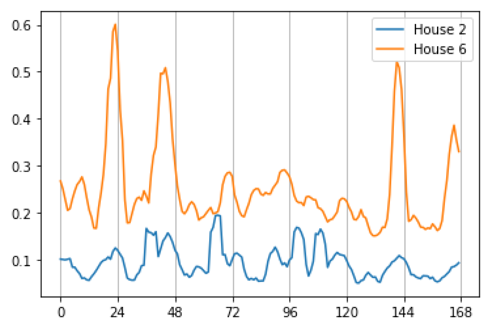
Figure 9.
Consumption behaviour for the centremost and farthest houses for the fourth week of 2016.

Figure 10.
Sensitivity analysis for combined factor variation.

Figure 11.
Sensitivity analysis for a set of activation functions combined: (a) factor influence; (b) general performance for activation functions combined with .
Figure 11.
Sensitivity analysis for a set of activation functions combined: (a) factor influence; (b) general performance for activation functions combined with .

Figure 12.
Factors combined and architecture performance for each factor: (a) variation of , (b) variation of , (c) variation of .
Figure 12.
Factors combined and architecture performance for each factor: (a) variation of , (b) variation of , (c) variation of .

Figure 13.
(a–aa) A box plot matrix showing results from DOE3. Each cell shows the architecture performance over the combined factor variation. Each boxplot was the result of five experiments with adjustments for h2 and h6. Box plots (a–c) show the architecture performance for , and . Variation over shows that experiments for (b) presents better accuracy with . Similar analyses were performed for columns and .

Figure 14.
Activation function sets combined with cases. Outer columns present the variation over : (a) performance with variation over , (b) performance over the three experiments.
Figure 14.
Activation function sets combined with cases. Outer columns present the variation over : (a) performance with variation over , (b) performance over the three experiments.

Figure 15.
Architecture evolution fitness curve for each activation function set (). For visualisation purposes, the first 50 generations were removed from the plot.
Figure 15.
Architecture evolution fitness curve for each activation function set (). For visualisation purposes, the first 50 generations were removed from the plot.

Figure 16.
Architecture performance for houses h2, h6 and h9: (a) CMA-ES adjusted weight performance, (b) average of results. For visual purposes, the first 140 generations were removed.
Figure 16.
Architecture performance for houses h2, h6 and h9: (a) CMA-ES adjusted weight performance, (b) average of results. For visual purposes, the first 140 generations were removed.

Figure 17.
Model performance for each house in the MH set: (a) root mean square error (RMSE), (b) mean absolute percentage error (MAPE), (c) accuracy.
Figure 17.
Model performance for each house in the MH set: (a) root mean square error (RMSE), (b) mean absolute percentage error (MAPE), (c) accuracy.


Table 1.
Similarity methods performance.
| Centremost House | Overall Performance for MH Similarity Set | ||||
|---|---|---|---|---|---|
| Similarity Method | House | MAPE (%) | Fitness | RMSE (kW/h) | MAPE (%) |
| Euclidean distance | 3 | 15.47 | −63.59 | 0.2939 | 14.80 |
| Cosine distance | 6 | 16.24 | −78.45 | 0.3477 | 17.94 |
| DTW distance | 2 | 13.41 | −58.92 | 0.2611 | 13.80 |
Table 2.
Description of parameters used during evolution.
| Parameter | Description |
|---|---|
| Population size of network agents. | |
| Maximum number of generations. | |
| Probability of inserting a node. | |
| Probability of adding a connection. | |
| Probability of changing an activation function. | |
| List of available activation functions. |
Table 3.
Settings for DOE 1.
| Factor | Distribution | Range of Values | Fixed Values |
|---|---|---|---|
| uniform | 0.25–0.75 | ||
| uniform | 0.25–0.75 | ||
| uniform | 0.25–0.75 |
Table 4.
Settings for DOE 2.
| Factor | Activation Function Set | Fixed Values |
|---|---|---|
Table 5.
Settings for DOE 3.
| Factor | Set of Values | Type of Variation |
|---|---|---|
| [0.25, 0.50, 0.75] | Combination | |
| [0.25, 0.50, 0.75] | Combination | |
| [0.25, 0.50, 0.75] | Combination | |
| Fixed |
Table 6.
Settings for DOE 4.
| Factor | Fixed Factor | Type of Variation |
|---|---|---|
| Combination with | ||
| Fixed | ||
| Fixed | ||
| Fixed |
Table 7.
Architecture evolution parameters.
| Parameter | Value |
|---|---|
| 320 | |
| Population | 100 |
| 0.25 | |
| 0.5 | |
| 0.25 | |
| = [, , , , ] |
Table 8.
Benchmark model parameters.
| Parameters | Feed-Forward NN | Vanilla LSTM | LSTM Features | LSTM One Shot |
|---|---|---|---|---|
| Number of features | 33 | 1 | 6 | 33 |
| Number of hidden layers | 2 | 1 | 2 | 2 |
| Number of node/layer | 20 | 5 | 12 | 20 |
| Best Epoch | 390 | 300 | 500 | 600 |
| Learning rate | 0.5 | 0.2 | 0.5 | 0.5 |
Table 9.
Load forecast evaluation summary.
| Average | Best House Avg | Centremost | Farthest | ||||
|---|---|---|---|---|---|---|---|
| Method | RMSE (kW/h) | MAPE (%) | Accuracy (%) | House | MAPE (%) | MAPE (%) | MAPE (%) |
| FFNN/2 h back | 0.0266 | 18.79 | 81.21 | h9 | 11.73 | 13.72 | 11.73 |
| FFNN/6 h back | 0.02742 | 20.47 | 79.53 | h10 | 11.66 | 16.18 | 20.31 |
| FFNN/12 h back | 0.0307 | 23.69 | 76.30 | h10 | 10.75 | 15.79 | 31.69 |
| Vanilla LSTM | 0.0253 | 16.67 | 86.83 | h2 | 12.07 | 14.01 | 14.21 |
| LSTM Features | 0.0235 | 14.92 | 85.08 | h7 | 11.16 | 13.73 | 17.27 |
| LSTMOS/2 h back | 0.0176 | 11.95 | 88.05 | h10 | 8.8 | 11.25 | 9.7 |
| LSTMOS/6 h back | 0.0175 | 11.94 | 88.06 | h2 | 8.58 | 10.18 | 10.34 |
| LSTMOS/12 h back | 0.0185 | 12.52 | 87.48 | h6 | 9.29 | 10.65 | 9.29 |
| DNN-CAE 2 | 0.017 | 8.77 | 91.23 | h7 | 6.56 | 9.44 | 8.96 |
Publisher’s Note: MDPI stays neutral with regard to jurisdictional claims in published maps and institutional affiliations. |
© 2021 by the authors. Licensee MDPI, Basel, Switzerland. This article is an open access article distributed under the terms and conditions of the Creative Commons Attribution (CC BY) license (http://creativecommons.org/licenses/by/4.0/).
Share and Cite
MDPI and ACS Style
Gomez-Rosero, S.; Capretz, M.A.M.; Mir, S. Transfer Learning by Similarity Centred Architecture Evolution for Multiple Residential Load Forecasting. Smart Cities 2021, 4, 217-240. https://0-doi-org.brum.beds.ac.uk/10.3390/smartcities4010014
AMA Style
Gomez-Rosero S, Capretz MAM, Mir S. Transfer Learning by Similarity Centred Architecture Evolution for Multiple Residential Load Forecasting. Smart Cities. 2021; 4(1):217-240. https://0-doi-org.brum.beds.ac.uk/10.3390/smartcities4010014
Chicago/Turabian StyleGomez-Rosero, Santiago, Miriam A. M. Capretz, and Syed Mir. 2021. "Transfer Learning by Similarity Centred Architecture Evolution for Multiple Residential Load Forecasting" Smart Cities 4, no. 1: 217-240. https://0-doi-org.brum.beds.ac.uk/10.3390/smartcities4010014