A Dynamic Mobility Traffic Model Based on Two Modes of Transport in Smart Cities

Abstract

This paper focuses on transportation models in smart cities. We propose a new dynamic mobility traffic (DMT) scheme which combines public buses and car ride-sharing. The main objective is to improve transportation by maximizing the riders’ satisfaction based on real-time data exchange between the regional manager, the public buses, the car ride-sharing and the riders. OpenStreetMap and OMNET++ were used to implement a realistic scenario for the proposed model in a city like Ottawa. The DMT scheme was compared to a multi-loading system used for a school bus. Simulations showed that rider satisfaction was enhanced when a suitable combination of transportation modes was used. Additionally, compared to the other scheme, this DMT scheme can reduce the stress level of car ride-sharing and public buses during the day to the minimal level.

1. Introduction

The mobility system in a city is an essential pillar for urban and modern development [1]. Currently, the forms of transportation (e.g., public and private) are incoherent and lack coordination, which makes them increasingly stressed. Moreover, as the human population grows, the vast increase in the number of vehicles on the roads leads to many challenges, such as traffic congestion and air pollution. These issues have a negative impact on the daily lives of citizens, business productivity, health and the environment. Today, government and city planners are focusing on building smart transportation solutions to optimize the use of transportation services and improve mobility in cities.

The concept of shared mobility based on new technologies can improve the reliability and efficiency of the traditional transportation system. Indeed, dynamic ride-share systems allow passengers to take other routes with the possibility of reducing a trip’s time and cost. At present, road network developers are focusing on integrating the two modes of transportation to provide the passenger with more dynamic transportation and on-demand mobility services [2].

In recent times, transit forms have developed significantly due to tremendous progress in the Internet of Things (IoT) with its ability to collect data in near real-time. At the same time, developments in computing technologies, vehicular communication and sensing make it possible for cars to very quickly inform their neighbors about traffic data.

Most of the previous studies, especially those carried out between 1999 and 2014 [3,4], focused on traditional ride-sharing schemes with a static itinerary, where the passenger shares his trip with other passengers with the same origin and/or destination.

The paper [5] proposed a combination of carpooling with public transport to obtain multi-mode mobility planning. The concept of the time-expanded model was applied to describe public transportation and carpooling networks. Merging public and carpooling networks presents fuzzy locations and flexibility for the road network. This model allows the user to use two modes of transportation on his trip from origin to destination.

This work is an extension of our previous work [6], in which we developed a dynamic scheme that enables riders to use cars or public buses, either exclusively or in combination during their trip, for the lowest fare and quickest time. At each station, passengers can be informed of the capacity of the public bus or car that will pass through the station, and their recent positions. In this contribution, we compare the dynamic mobility traffic (DMT) model with another model in [7] to show that our scheme is a more suitable choice and affordable option for passengers. The most relevant work presented by reference [8] has proposed a framework for multi-modal transportation networks based on prediction schemes to improve the urban transport. The model consists of three layers of the transportation networks with different coverage ranges in three different cities. We note that this model does not consider the time and cost required for the trip.

The contributions of this work are summarized as follows:

• A new dynamic mobility traffic (DMT) model was formulated based on the game-theoretic scheme.
• A new algorithm is proposed to manage riders’ needs in terms of mobility service. For each rider, optimal transportation planning is provided, whether by public bus, car or both, to reach their goal in a reduced time and at the lowest possible cost.
• Simulations were run to evaluate the developed scheme.
• A comparison with a multi-loading system introduced proposed in [7] proved the efficiency of the DMT.

The rest of the paper is presented as follows. Section 2 surveys recent publications related to our work. Section 3 describes the methodology of the DMT model. Section 4 formulates and explains the DMT algorithm. Section 5 details the simulation process of the DMT model. Finally, Section 6 provides some concluding remarks.

2. Related Work

Currently, research related to the smart city concept for the intelligent transportation system (ITS) has focused on how to decrease CO2 emissions, travel costs and travel time. The ridesharing optimization problem focuses on finding the shortest path or the shortest trip interval to arrive at one’s destination [9,10]. This optimization leads to enhancing the quality of life of the person who uses car ride-sharing or a public bus to travel within a city. In this section, we review previous studies of intelligent dynamic mobility-traffic systems developed by integrating ride-sharing and public transit models.

Many studies in the last decade have focused on route planning in transportation networks. The authors in [11] outlined the essential techniques used to create a multi-mode transportation system. This study addressed some algorithms for calculating the shortest paths of road networks and performance metrics related to dynamic road networks [12,13].

When we combine several network graphs into a single graph and then apply the routing algorithm, we obtain a multi-modal route plan. The system in [14] is a piece of multi-modal technology that does not require the passenger to specify restrictions on the use of different modes of transport prior to the start of the trip. For example, the passenger can travel by car and then decide to take the bus. This model differs from [15], which uses the nearest neighbor algorithm since the processing time is faster. In addition, the system is implemented so that it can solve any inquiry locally. In [16], the authors created a multi-modal routing system based on previous information stored in the user’s profile with a range of possible travel options. This work aims to reduce complications and computational effort for the multi-modal transportation model through the use of heuristic schemes.

Some works are based on ride-share route planning strategies, but with specific limitations, such as common destination and origin. In general, these problems are either single-origin-multi-destination or multi-origin-multi-destination scenarios. In [17], a model was developed that calculates the shortest route and best cost for a single-origin-multiple-destination trip. In fact, multi-origin-multi-destination trips are considered more complex than single-origin-multi-destination trips [18,19]. Ref. [18] suggested a new technique for calculating the shortest ride-share route to reach the target with optimization constraints. The route would be changed to meet each request, and then the appropriate route change restrictions would be computed. Ref. [19] used a hybrid simulated annealing model to create a system for passengers requiring dynamic/online carpooling. This new technique requires complex calculations, especially when the number of requests is large. These complex calculations lead to a vast number of repetitions and multiple random disturbances.

Similarly, many studies have developed methods to identify meeting points for car drivers and riders [20,21]. Ref. [20] aimed to build a dynamic, decentralized and integrated system that maintains the privacy of the passenger. The meeting points are calculated in the ride-sharing service so that each user can continue to control their location information. In [21], a new site-based system was proposed for suggesting meeting points for passengers and drivers in the real world. In this scenario, it is assumed that the driver drives his car through the city’s main streets to be able to pick up one or more passengers from a single meeting site. At the same time, passengers are expected to walk or use public transport to reach the agreed assembly point.

In addition to the ride-sharing transportation mode, advanced transportation systems are concerned with the development of dynamic public transport and bicycle sharing in smart cities. The model in [22] is based on the idea that the search for the shortest route of public transport should be reduced to a specific area for each car after filtering the requests that would reduce the quality of service provided to the passenger. This system works by creating an efficient path planning greedy algorithm strategy that helps speed up complex calculations.

In [23], a mobility system was established to combine carpooling and traditional multi-modal transportation in the same trip in real time. The basic idea here is based on the principle of replacing some sub-routes on the traditional multi-modal transport route with carpooling paths. The intention is to reduce the passenger’s travel duration. This work is a development based on [24]. Here, the system focuses on the number of stations rather than the number of potential drivers. This concept helps reduce the number of launched Dijkstra algorithms. Most modern transportation systems create multi-origin-multi-destination strategy transportation models with sophisticated search techniques and lots of information uploaded to the cloud. Reference [25] targets dynamic multi-network mobility in urban areas. The research suggests a model to find solutions for traffic flow with the participation of carpooling, public buses and trains within the framework of a single traffic system. The developers in [26] designed a mobile platform that offers suggestions for planning a trip that includes only two modes of transport, including carpooling and public buses. This solution ensures the shortest route for the passenger while considering delays caused by road accidents and traffic congestion. In [27], the purpose of the system is to combine two modes of transportation (ride-sharing and car-sharing) in one model so that the passenger can operate the multi-trip scheduling as one task. We note the shortcomings in this work. Most modern models focus on only one aspect, for example, reducing time without taking into account lowering costs. Additionally, the paper focuses on one or two modes of the transportation system without considering the diversity in terms of user needs.

In [7] a multi-loading school bus routing model with four meta-heuristics was applied to solve a new complexity in the multi-loading issue. The older version permits students from various schools to ride the same bus at the same time. However, the scheme in this paper enables the bus to take students to or from school simultaneously. This model gives us lower cost transportation with flexible routing.

Contrary to our work, most current mobility traffic schemes are static and focus on a single form of transportation. Our work includes a suitable model for users to select either one transport mode or a combination of two transit modes for their trip with the lowest fare and the shortest period.

3. Model Overview and Methodology

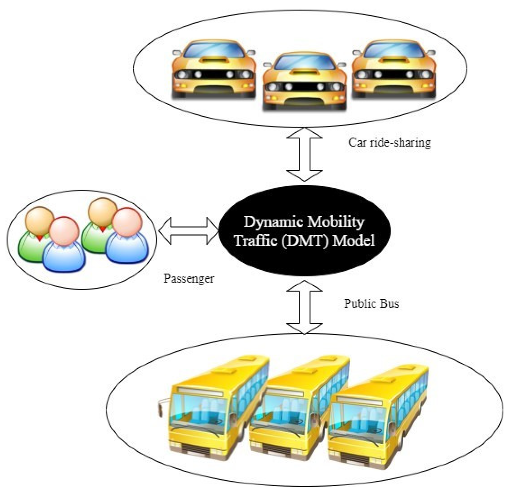
Figure 1 shows the main components of the DMT model, consisting of car ride-sharing, public buses and passengers. In this model, costs differ depending on the distances traveled by the passengers to reach their destinations. We assumed several relevant hypotheses that must be mentioned. First, we did not consider the person’s walking time between the stations in his trip. Second, the passenger’s origin is the first station of the journey and the last station is the destination. Finally, security and trust have been assumed in this model.

3.1. Public Bus Methodology

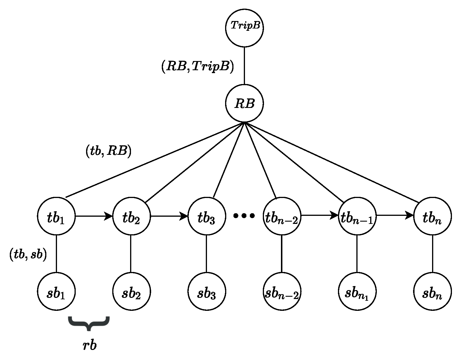
The public bus schedule determines the route of each vehicle and the time required to reach the destination. The schedule usually consists of a set of stations ($SB$), a set of buses (B), a set of time ($TB$) and a set of routes ($RB$). All the above parameters can be written as $SCB=\{SB,B,TB,CB\}$. A route $rb\in RB$ can be written as $rb=\{b,ssb,tsb,sdb,tdb,cb\}$. Here, a bus is $b\in B$; the starting station is $ssb$ and the destination station is $sdb\in SB$; the departure time is $tsb$ and the arrival time is $tdb\in TB$; and the bus capacity on each route is $cb$. Figure 2 represents a time-expand model of a public bus network. The trip is composed of a sequence of time nodes ($tb$) at different stop nodes ($sb$) and it belongs to a route $RB$. Here, $TripB$ is node contains a set of trips.

3.2. Car Ride-Sharing Methodology

In the car ride-sharing, $RC$ is a set of user requests at a given time $tc$. C represents a group of vehicles that have a specific capacity ($cc$) and a set of stations ($SC$). Here, the starting station is $ssc$, and the destination station is $dsc\in SC$; the maximum waiting time is $max\_w$; the acceptable time detour in the trip is $\eta$; and $n\_r$ is the number of riders. The trip request is expressed as $RC=\{c,ssc,dsc,max\_w,\eta ,n\_r\}$. Figure 3 represents a time-expand model of a car ride-sharing network. A trip is composed of a sequence of time nodes ($tc$) at different stop nodes ($sc$) and it belongs to a route $RC$. Here, $TripC$ is node contains a set of trips.

The scheduling process for cars and public buses defines their routes and destination times. We assume that the passenger (r) periodically receives information describing the current positions of ride-sharing cars ($l_{c,n}$) and the buses’ positions ($l_{b,n}$) with their seating availability. This information, which is collected based on a passenger’s preference (P) for bus, car or both, is used to calculate the total price ($T{P}_i$) and the total travel time ($T{T}_i$). More details are presented in Section 4 and Section 5.

This proposed model allows each passenger to choose vehicles (ride-sharing car and/or public buses) that they want to take according to their preferences in terms of maximum arrival time ($T{T}_{max}$) and maximum cost ($T{P}_{max}$).

4. Problem Formulation: A Dynamic Mobility Traffic Model

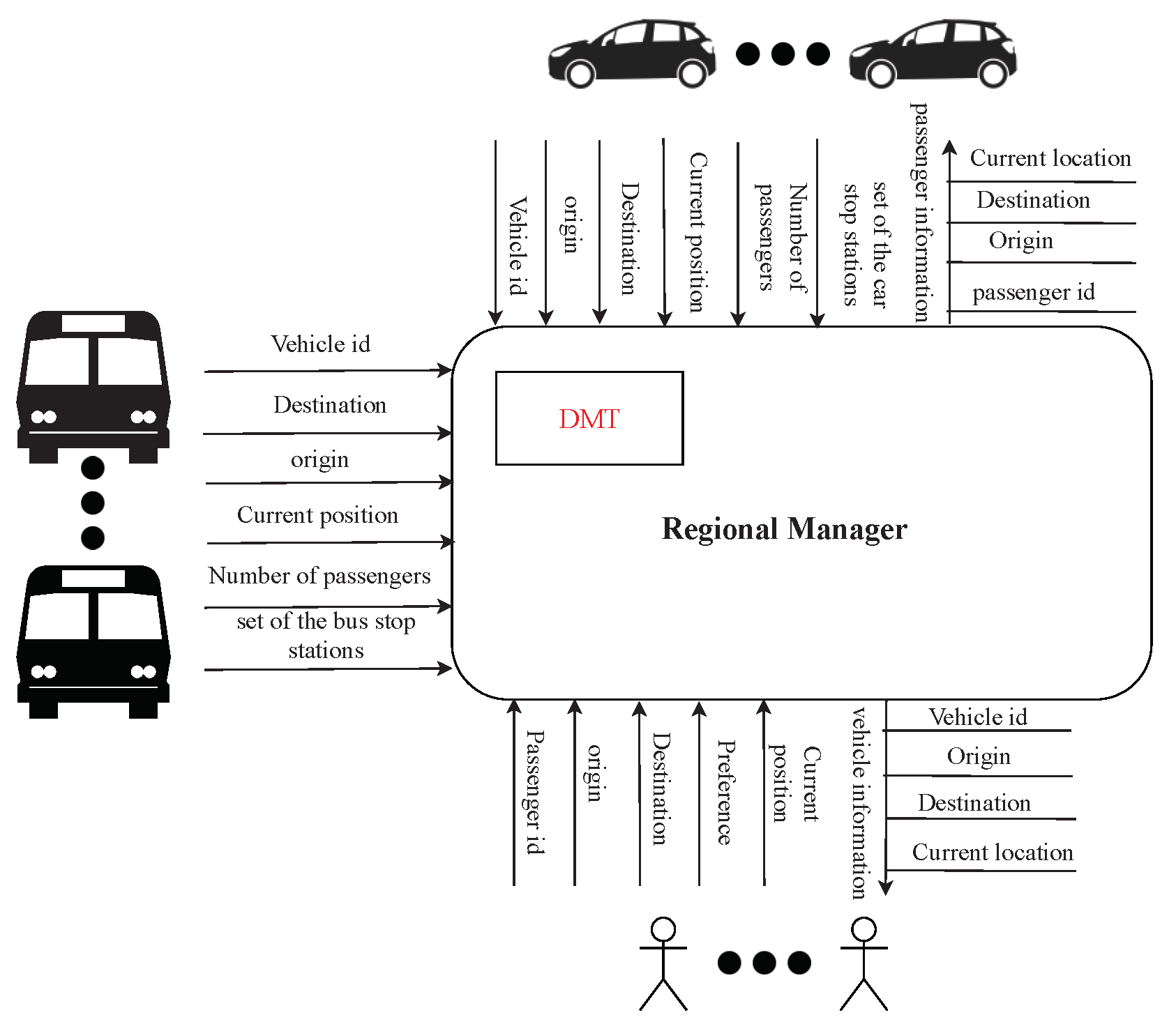
This section explains the algorithm and mathematical equations that are used to implement the DMT model. We assume that the DMT manager receives updated information from all participants every 5 min. As we can see, Figure 4 shows the main interaction between the players in the model. Each element has a set of parameters that contribute to the implementation of the logarithm of the proposed model. In this figure, the regional manager uses the DMT to manage the interconnection between the car ride-sharing, the public bus and the passenger.

Table 1. Public bus notation and definitions.

Notation	Definition
$cb$	The maximum public bus capacity
$TT(l_{b,n},s{b}_i)$	The total trip period from the recent location of the public bus to the current station of the rider
$l_{b,n}$	Current location of the public bus
$s{b}_i$	The current rider station
$SB$	Set of stations in the public bus schedule
B	Set of public buses
$TB$	Set of departure and arrival times for the public buses
$RB$	Set of routers for the public buses
$SCB$	Set of public buses schedule
b	The public bus identity
$ssb$	The origin public bus station identity
$sdb$	The destination public bus station identity
$\alpha$	The time constraint for a public bus trip
$tsb$	The time in the origin public bus station
$tdb$	The time in the destination public bus station
$rb$	The public bus route
$WT{B}_j$	the total waiting time in a public bus station
$TP{B}_i$	The total fare of the public bus trip
$TT{B}_i$	The total period time of the public bus trip
$TT{B}_j$	the total time from the source station to the destination station

,

Table 2. Car ride-sharing notation and definitions.

Notation	Definition
$RC$	Set of car ride-sharing requests
$SC$	Set of car ride-sharing stations
C	Set of cars
c	The ride-sharing car’s identity
$cc$	The capacity of specific car
$ssc$	The start car station identity
$dsc$	The destination car station identity
$\eta$	The acceptable time detour
$TT(l_{c,n},s{c}_i)$	A time from the current location of the car to the current station
$l_{c,n}$	Current location of the car
$s{c}_i$	The current rider station
$tc$	The requested car ride-sharing time
$WT{C}_j$	The total waiting time in a car ride-sharing station
$TP{C}_i$	The total fare of the car ride-sharing trip
$TT{C}_i$	The total period time of the ride-sharing trip
$TT{C}_j$	The total time from the source station to the destination station

and

Table 3. Trip notation.

Notation	Definition
$s{s}_i$	The origin rider station
$d{s}_i$	The destination rider station
$T{T}_i$	The total trip time
$T{P}_i$	The total trip price
$n\_r$	The number of the riders
$i\in R$	Each rider i belongs to R
R	Set of riders
$\sigma$	The acceptable detour distance in the trip
$D(s{s}_i,d{s}_i)$	The shortest distance between the origin and the destination
$TD(s{s}_i,d{s}_i)$	The total distance of the trip
$T{P}_{Max}$	The maximum price
$T{T}_{Max}$	The maximum time
$max\_w$	The maximum passenger waiting time
P	The rider preference

define the parameters of the model in this paper. The DMT is an optimization problem, and the following mathematical equations are used to establish the optimization task for this model.

According to the methodology of the car ride-sharing and of the public bus from the previous section, the cost (time and price fare) optimization problem is expressed as:

$$\underset{i\in R}{\mathrm{minimize}}\{T{P}_i,T{T}_i\}$$

(1)

subject to:

$$n\_r⩽cc$$

(2)

$$n\_r⩽cb$$

(3)

$$TT(l_{c,n},s{c}_i)⩽max\_w$$

(4)

$$TT(l_{b,n},s{b}_i)⩽max\_w$$

(5)

$$\begin{array}{c}\hfill \sigma *D(s{s}_i,d{s}_i)⩾TD(s{s}_i,d{s}_i),\\ \hfill s_i\in SB\cup SC\end{array}$$

(6)

$$T{P}_i⩽T{P}_{Max}$$

(7)

$$T{T}_i⩽T{T}_{Max}$$

(8)

Equations (1)–(8) can has seen as a game theory system in which all participants (passenger, ride-sharing car and public bus) want to maximize their interests.

From the above equations: (1) $T{P}_i$ is the total price of the trip for a particular rider; (2) $T{T}_i$ is the whole journey time for the rider; (3) $n\_r$ is the number of passengers on the trip; (4) $cc$ and $cb$ are the ride-sharing car’s and the public bus’s capacities, respectively; (5) $TT(l_{c,n},s{c}_i)$ and $TT(l_{b,n},s{b}_i)$ are the total trip period from the current location of the vehicle to the existing station of the rider for the car and public bus, respectively; (6) $\sigma$ is the acceptable detour distance in the trip; (7) $D(s{s}_i,d{s}_i)$ is the shortest distance between the origin ($s{s}_i$) and the destination ($d{s}_i$); (8) $TD(s{s}_i,d{s}_i)$ is the total trip distance; (9) $T{P}_{Max}$ is the maximum trip price; (10) $T{T}_{Max}$ is the trip time.

The distinctive feature of the DMT scheme is the objective function (1) and its constraints, which determine the minimum value of trip time and trip price. The restriction numbers (2) and (3) indicate that the numbers of passengers must not exceed the maximum numbers of seats in the buses and cars, respectively. In this model, the actual pick-up time should not be more than the maximum waiting time for riders at each car and bus station (constraints (4) and (5)). Constraint (6) shows that the total distance between the originating station and the destination station must be equal to or less than the product of the acceptable detour distance and the shortest distance between them. Constraint (7) cost of the trip must not exceed the maximum amount that the user can pay, while constraint (8) ensures that the time taken for the trip is less than the maximum time that the user wishes to be on the trip.

$$T{T}_i=TT{B}_i+TT{C}_i$$

(9)

The total trip time is the sum of the whole time when the rider uses the public bus ($TT{B}_i$) and the entire time when the rider uses the car ($TT{C}_i$) on the same trip.

$$\underset{i\in R}{TT{B}_i}=\sum _{j=1}^{d{s}_j}TT{B}_j+WT{B}_j+\alpha$$

(10)

Equation (10) calculates the entire trip time when the rider uses the public bus. It is the sum of the total trip time from the source to the destination ($TT{B}_j$) and the waiting time at each station ($WT{B}_j$) and a time constraint for a public bus $\alpha$.

$$\underset{i\in R}{TT{C}_i}=\sum _{j=1}^{d{s}_j}TT{C}_j+WT{C}_j+\eta$$

(11)

Equation (11) calculates the entire trip time when the rider uses the car ride-sharing. It is the sum of the total trip time from the source to the destination ($TT{C}_j$) and the waiting time at each station ($WT{C}_j$) and a time constraint for car ride-sharing trip $\eta$.

To calculate the total price, we use the following equation:

$$T{P}_i=TP{B}_i+TP{C}_i$$

(12)

where

$$TP{B}_i=xdollar*TT{B}_i/hour$$

(13)

Equation (13) calculates the total price of the bus trip. In the City of Ottawa, for example, the bus fare for each passenger is 3.5 Canadian Dollars per 90 min.

$$TP{C}_i=Y*TTC/TT{C}_i$$

(14)

Equation (14) calculates the total car ride-sharing price for each passenger. It is calculated by dividing the entire passenger’s trip time when using carried-sharing ($TTC$) by the total trip time for all passengers ($TT{C}_i$) multiplied by the total cost for the ride-sharing.

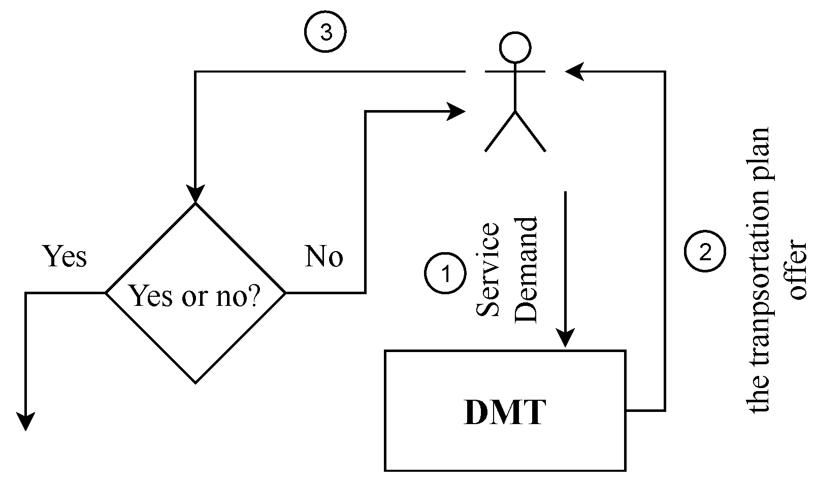
We assume that all public buses and ride-sharing cars are connected to a mobile application to track all participants in real time. We propose the DMT algorithm to manage the demand for the transport service. Upon receiving periodical information about the availability of public buses and cars (available seats and time to reach the station), the DMT calculates the time required by each available vehicle (having empty seats) to arrive at the final destination from the passenger’s current position. It schedules the results in descending order. The result is compared to the passenger’s maximum arrival time, and the first public bus with an equal or lower value will be selected. In order for the passenger to determine whether to continue to traveling on the same public bus or transfer to another bus, the time required to reach the destination on the recent bus is compared to the result of the previous process. The passenger chooses a public bus in the shortest possible time. The same process occurs if a ride-sharing car is selected as the mode of transportation for the whole trip.

On the other hand, the passenger can choose to use a combination of the public bus and car ride-sharing on his trip. The model gives him the optimal combination with the fastest arrival time and the least cost. Figure 5 shows the interactions between a user and the DMT model.

5. Simulation and Results

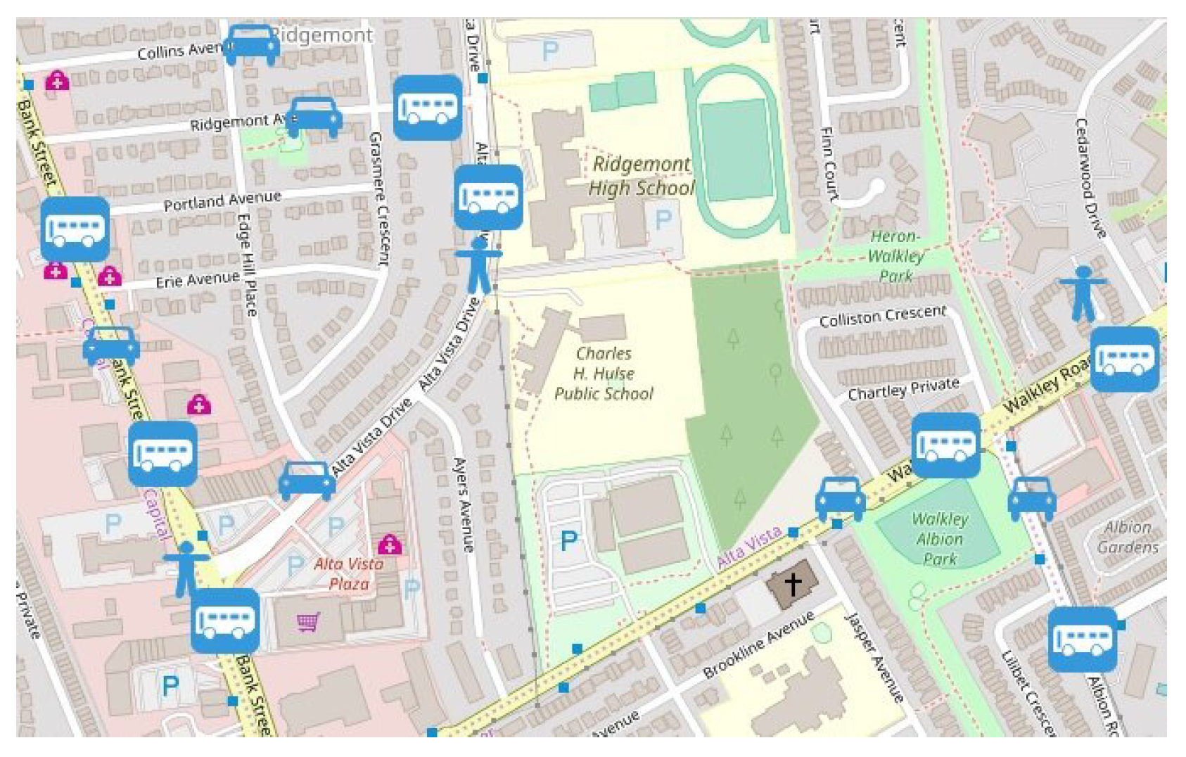
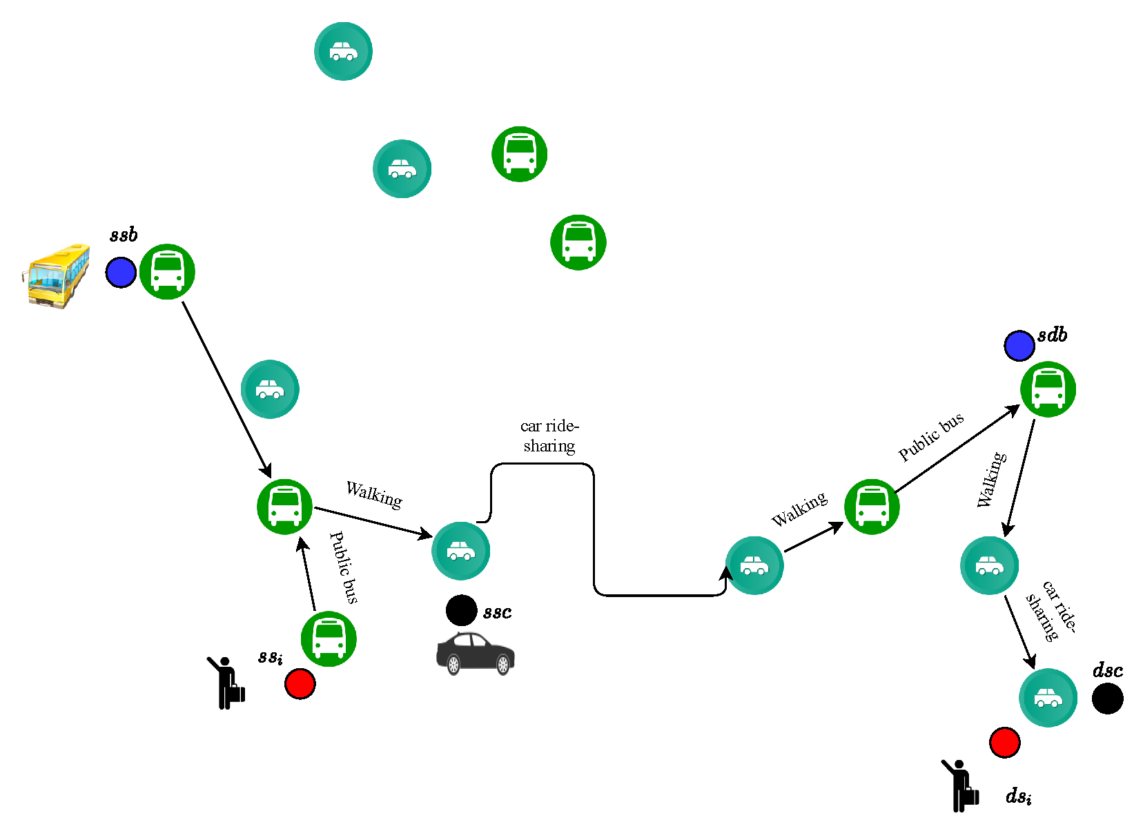
Table 1, Table 2 and Table 3 show the parameter notation used in this work. Figure 6 shows the partial map of the City of Ottawa with two forms of transportation (public buses and car ride-sharing). In Section 5.2, we evaluate our model (DMT); then we compare the performance of DMT in Section 5.3 with a multi-load model presented in [7]. Figure 7 presents an example of a passenger’s route from the origin to the destination (public bus–walking–car–walking–public bus–walking–car). The figure is another representation of Figure 4, a map used in this work with the locations of car and bus stations for a part of the City of Ottawa. The red, blue and black dots represent the departure and arrival points for one passenger, one bus and one ride-sharing car respectively.

5.1. Simulation Setup

In our testing, the route journey was built using Simulation of Urban Mobility (SUMO) and OMNET++ programs. In addition, we used OpenStreetMap (OSM) to extract a part of a map of the City of Ottawa as a case study. By extending $Inet$ and $Veins$ modules, which are written in C++, the module interfaces and protocol messages have been implemented. $Venis$ was used to realize the transportation mobility environment and $Inet$ framework to build a Wifi network. Additionally, the researchers connected $Veins$ with SUMO to create the random mobility scenario.

Table 4. Simulation of Urban Mobility (SUMO) parameters.

Parameters	Values
Vehicle Type	Car ride-sharing, Public bus
Road Network	NETCONVERT
Time Period to Simulate	6 a.m–11:59 p.m
Length of Time Step	1 min
Dimension of Simulation Area	20 km × 20 km
The Integration Method	Euler Update

and

Table 5. Simulation parameters.

Parameters	Values
$n\_b$	10 public buses in the simulation
$n\_c$	10 cars in the simulation
$n\_r$	40,000 passengers
$ns\_b$	30 public bus station
$ns\_c$	20 car ride-sharing station
$cb$	50
$cc$	4
Simulation Period	6 a.m.–11:59 p.m.
P	=1 If a public bus only
	=2 If a car only
	=3 If a public bus and car

indicate the SUMO values and the simulation parameters, respectively. At the same time, Figure 8 and Figure 9 show the output plots (average user satisfaction and stress level of using a public bus and car ride-sharing), which were drawn by MATLAB. In the simulation, the mobility traffic in the city was created randomly using SUMO, which included the traffic of public transport buses, cars and passengers from 6 a.m. to 12 p.m.

5.2. Dynamic Mobility Traffic (DMT)—Experimental Evaluations

From 6 a.m. to 11:59 p.m., the simulation was run by adjusting some parameters of the public buses and the cars during the trip, such as the number of public buses ($n\_b$) to 30, the maximum capacity of a public bus ($cb$) to 50 passengers, the number of bus stations ($ns\_b$) to 30, the number of cars ($n\_c$) to 10, the maximum car ride-sharing capacity $cc$ to four passengers, and the number of car stations to 20. In addition, we set the number of passengers ($n\_r$) to 1000 and assigned the route for each passenger from the departure station ($s{s}_i$) to the destination ($d{s}_i$). The public bus fare was calculated at C$3.50 for an hour and a half, and the rate when using the Uber taxi was estimated at C$1.74/min. The passenger chose his/her preferred mode of transportation (a public bus, car ride-sharing or a combination of a bus and car). In this work, the maximum arrival time and the maximum price were determined randomly by the simulation.

5.2.1. A Comparative Analysis

In the DMT model, user satisfaction is the number of passengers who accept the trip plan (source, destination, price, trip time, bus and car ride-sharing scheduling) as suggested by the DMT system after sending the demand divided by the total number of passengers in the simulation. At the same time, the stress level is the number of transportation modes (car and bus) used by the passengers divided by the total number of vehicles in the simulation.

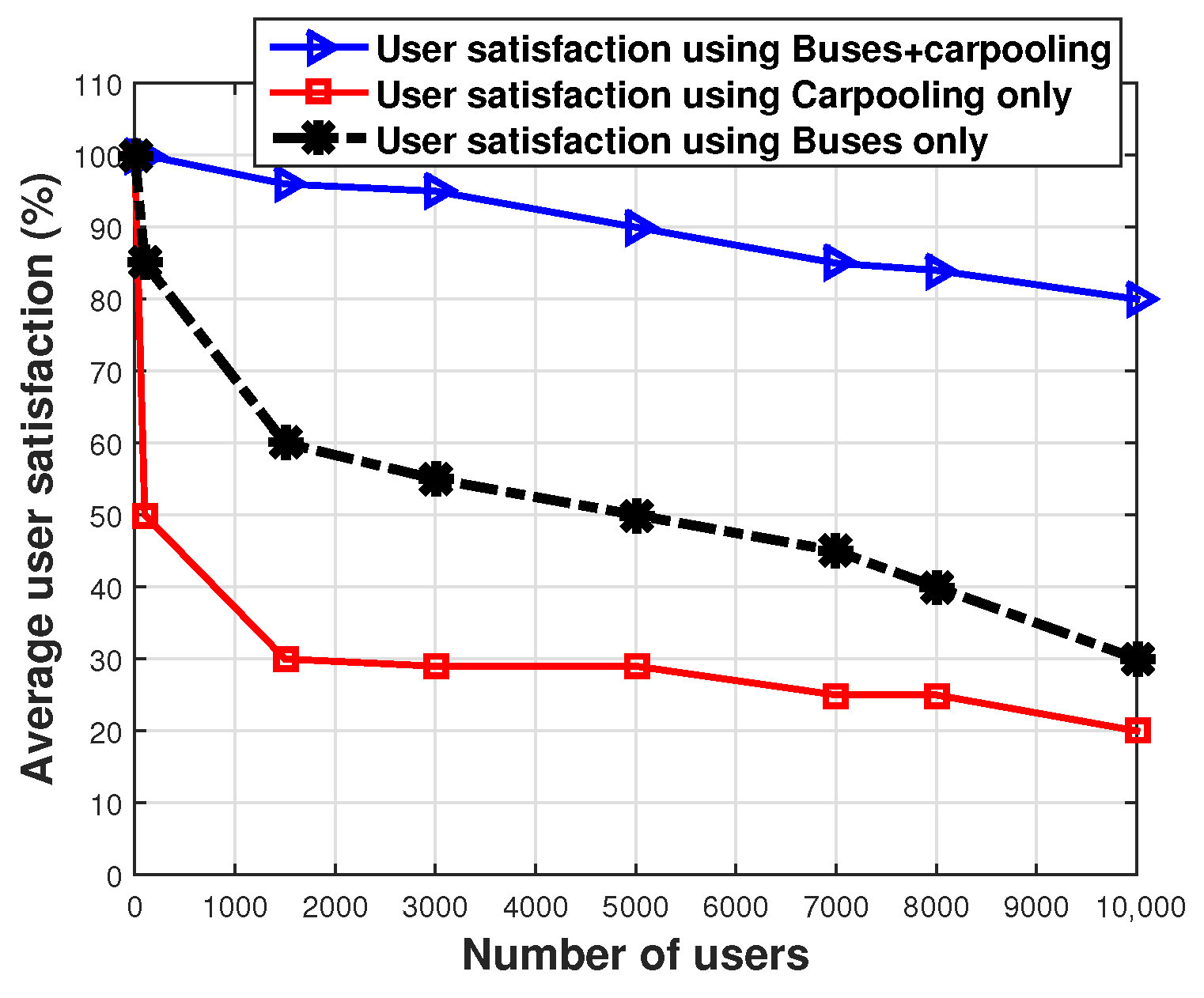
It can be seen from Figure 8 that the satisfaction rate of passengers using any mode of transportation decreases with an increase in the density of users. The average user satisfaction when using only buses or cars is less than the average user satisfaction when using a combination of car ride-sharing and public buses. The savings rate for car ride-sharing when the number of users is equal to 1500 is 68.42%, and for the public bus it is 36.8%, as shown in

Table 6. Savings rate of the average user satisfaction in the case of using a public bus only.

Passenger Number	Public Bus and Car Ride-Sharing (%)	Public Bus Only(%)	Saving Rate (%)
[1–1500]	95	60	36.8
[1501–7000]	85	45	47.06
[7001–10,000]	80	30	62.5

and

Table 7. Saving rate of average user satisfaction in the case of using a car ride-sharing only.

Passenger Number	Public Bus and Car Ride-Sharing(%)	Car Ride-Sharing Only (%)	Saving Rate (%)
[1–1500]	95	30	68.42
[1501–7000]	85	25	70.6
[7001–10,000]	80	20	75

. This ratio remains almost unchanged in the case of 7000 users, but differs when the number of passengers is equal to 10,000. In the case of 10,000 passengers, the savings rate is 75% for the car ride-sharing only, and almost 62.5% for riding the public bus only.

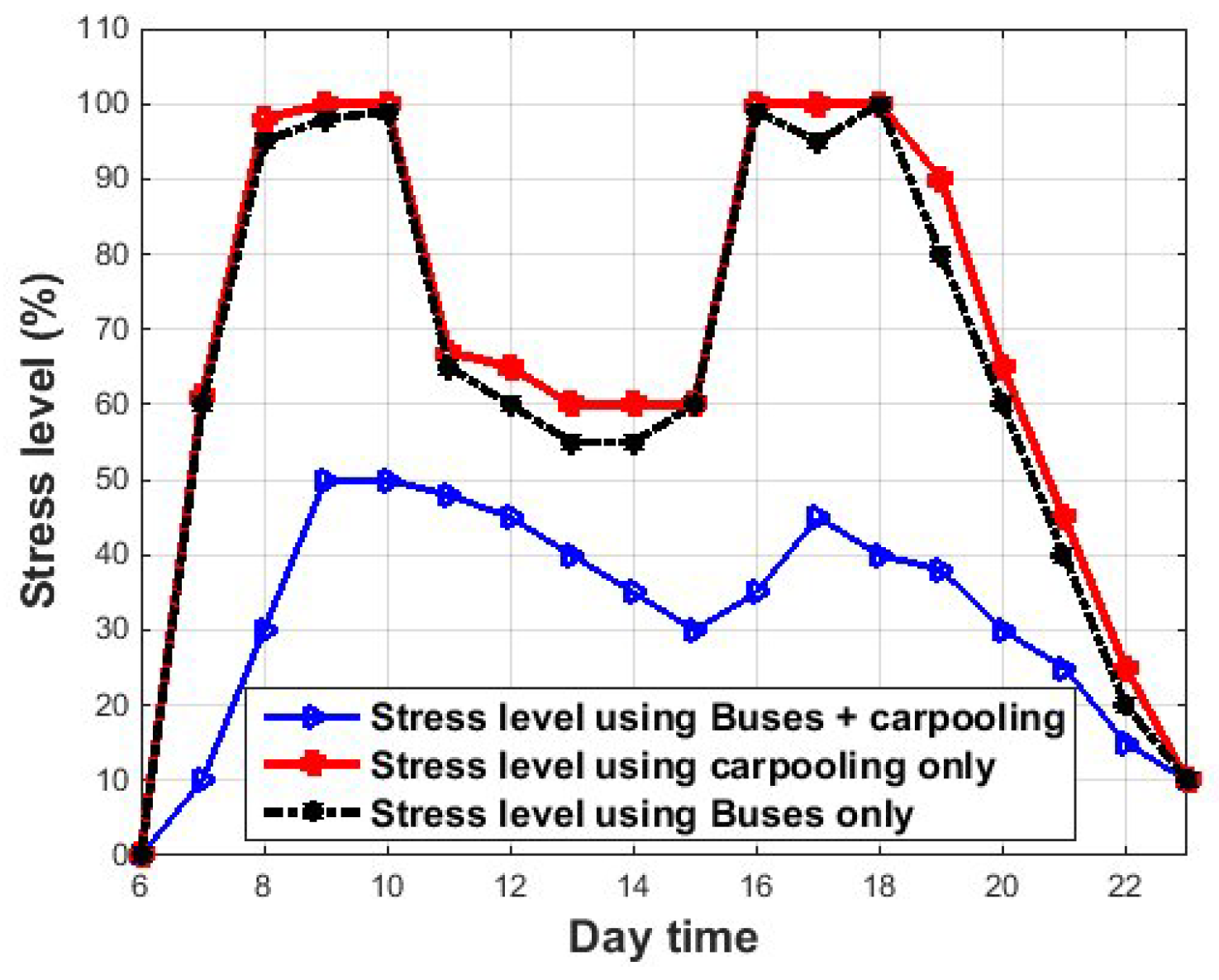
Figure 9 compares the stress level of passengers when using various modes of transportation from 6 a.m. to 11:59 p.m. The figure shows that the stress levels when using only the public bus or only the car ride-sharing are very similar. The stress level increased significantly from 6 a.m. to 8 a.m. It then decreased, and increased during the day until 6 p.m. At 6 p.m., the stress level was 95%, after which the percentage began to drop to 10%. If we compare the savings rate when using the ride-sharing car or public bus with that only using the car and bus together, we find that the price savings increased from 6 a.m. until it reached 45% at 10 a.m. Next, the conservation rate decreased very significantly to reach around 15% at 11 a.m. From 11:01 a.m., the same ratio continued to rise to 60% at 4 p.m. before the rate began to decline significantly after 6 p.m. to 0% at 11 p.m. From

Table 8. Savings rate of average stress level in the case of using a public bus or car ride sharing.

Day Time	Public Bus and Car Ride-Sharing (%)	Car Ride-Sharing or Public Bus (%)	Saving Rate (%)
[6:00 a.m.–11:00 a.m.]	49	65	24.6
[11:01 a.m.–3:00 p.m.]	30	60	50
[3:01 p.m.–11:59 p.m.]	10	10	0

, we found that the savings rate between 6:00 a.m. and 11:00 a.m. is 24.6% when using the public bus or car ride-sharing. This ratio increased until 3:00 p.m., at which time the savings rate was 50% for riding in a car or a public bus. However, it was equal to 0 at 11:59 p.m.

5.2.2. Results and Discussion

As shown in Figure 8, it is evident that the user satisfaction level using only a car to travel is lower than the user satisfaction level when using only a public bus. This result can be illustrated as follows. The percentage of users who express satisfaction when using a bus is higher, especially since buses have more seats than cars. The explanation for this result is that the DMT scheme’s concept is based on how the user reaches his destination for the lowest possible price and in the shortest possible time, regardless of other luxury preferences or congestion factors while riding. Besides, the satisfaction ratio is the percentage of satisfied users to the rate of dissatisfied users.

It can be seen from Figure 9 that during the rush hours, the ratio of the stress level ascends, illustrating the rate of the high-stress when using any transport mode between 7 and 10 a.m. and then between 3 and 6 p.m. In addition, we noticed that the stress level is lower when using two transportation modes together compared to the stress level when using only one transportation mode. By providing this feature, DMT not only reduces the time and fare for the user to arrive at his destination, but also helps to encourage commuters to use car ride-sharing, reduce the amount of manufacturing, and put pressure on governments to reduce the cost of running a vast number of buses. Thus, this can ultimately minimize the environmental damage caused by the use of a huge number of public buses with their correlated GHG emissions and reduce the government’s transportation budget.

5.3. Comparison between DMT and a Multi-Load Model

To prove the effectiveness of our proposal, we compare our DMT performance with the heuristic multi-load model, which is presented in [7].

5.3.1. A Multi-Load System Overview

The authors in [7] developed a new mechanism to deal with the multi-load school bus routing problem. This mechanism is the advanced version of the mixed load model. The mixed loading theory solves the bus routing problem in which students from different schools use the same bus at the same time. On the other hand, the multi-load model allows students from different schools and in different periods (morning, afternoon, evening, and full-time) to ride the same bus, regardless of whether the students are being taken to school or brought back home.

The main objective in [7] is to build a model with a reduced daily cost of routing in the city. According to statistical data from the Brazilian government, the charge is approximately 36 million U.S. Dollars annually when using a mixed load model or 34 million U.S. Dollars annually when using a multi load model. Four heuristics, each created using a different Iterated Local Search, have been developed to determine which mechanism will yield the best result. The first heuristic (H1) is called classic ILS with a normal local search.

On the other hand, the second heuristic (H2) adds a new local search called SmallVRPTW to the set of neighborhood structures. In the third heuristic (H3), the authors used an elite set with a diversification strategy to avoid the local optima problem. Finally, the fourth heuristic (H4) contains more smart criteria to decide the following: (1) which solution to use in the VND loop, (2) which solution to remove from the elite set, and (3) when to add a solution to the elite set.

For perturbation, (1) classic perturbation is used in H1, and (2) trip perturbation is used in H1, H2, H3, and H4.

A simulation was implemented to evaluate and compare these four heuristics, using real data from school bus routing in Espírito Santo, Brazil, within 12 h, regardless of whether students were going to school or returning home. Based on the results, the authors conclude that H4 is superior to the other three heuristics in terms of the least cost and the shortest travel time for transporting passengers, since it saves approximately two 2 million USD.

5.3.2. Main Differences between DMT and a Multi-Load Model

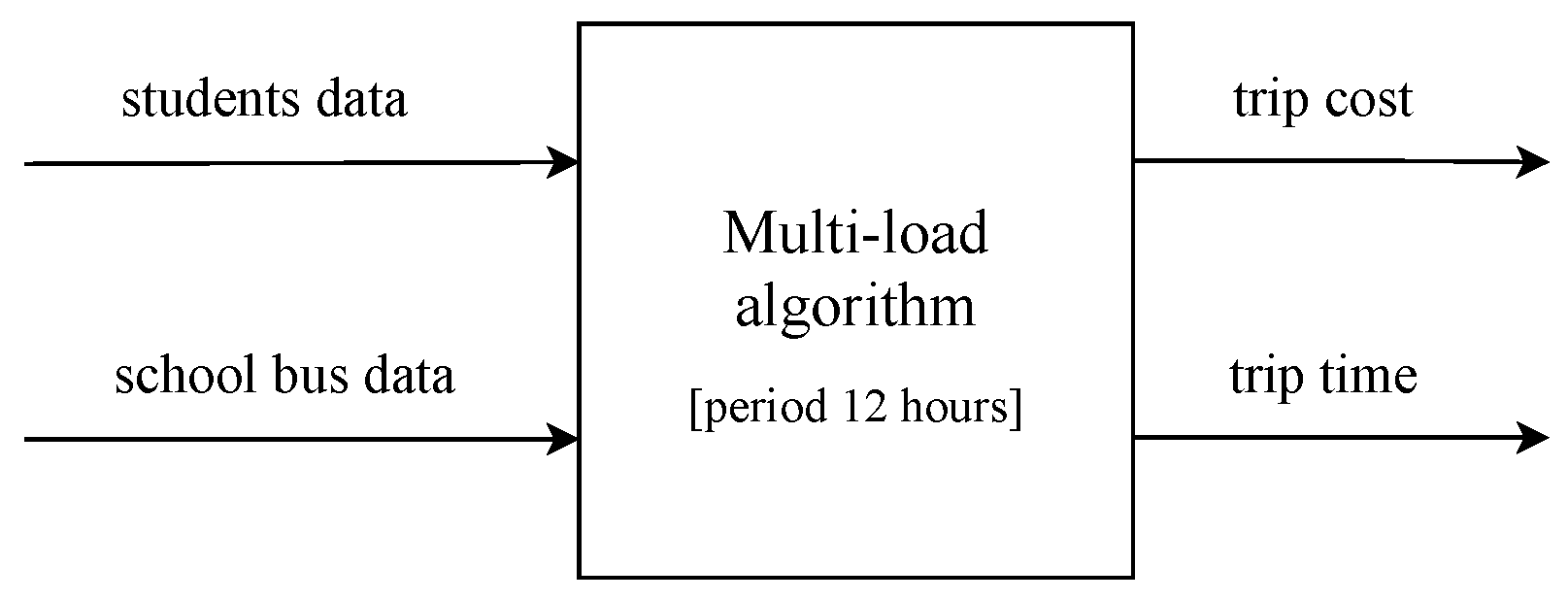
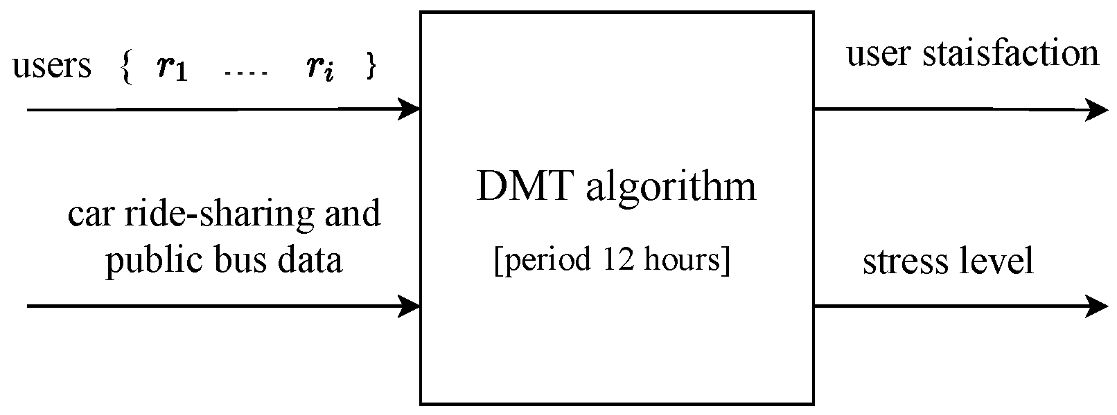
Although the work in [7] and our work in this paper both focus on finding a more cost-effective and less time-consuming model for travellers within cities, there are fundamental differences between them. First of all, H4 is based only on the school bus, while DMT is based on the bus and car ride-sharing, thereby providing passengers with more options to reach their destinations. Secondly, H4 deals with constant data for bus movement and student mobility. It is different from the DMT model, which depends on the dynamic information about the presence of public bus and car ride-sharing. As mentioned earlier, the passenger receives instantaneous data about the movement and place of the vehicle during the trip. Thirdly, the output of H4 is calculated based on the average values of time and cost for the bus trip within 12 h. At the same time, the DMT relies on the model’s dynamic information within 24 h to calculate the satisfaction of each passenger immediately after the trip ends. Figure 10 and Figure 11 show the inputs and outputs of multi-load model and the DMT, respectively.

We re-ran the multi loading logarithm in [7] using MATLAB from 6 a.m. to 11:00 p.m., and here we compare the results with those obtained from our work (DMT). In the multi-loading, user satisfaction is the number of students who arrived at their destinations without delay divided by the total number of students. At the same time, the stress level is the number of school buses used by the students divided by the total number of buses in the simulation.

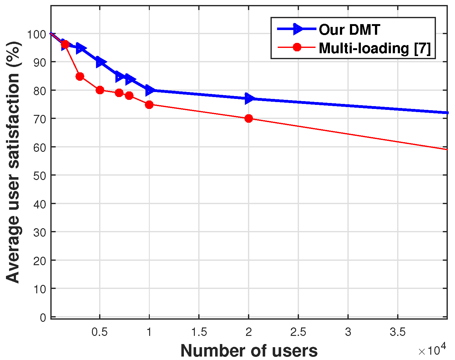
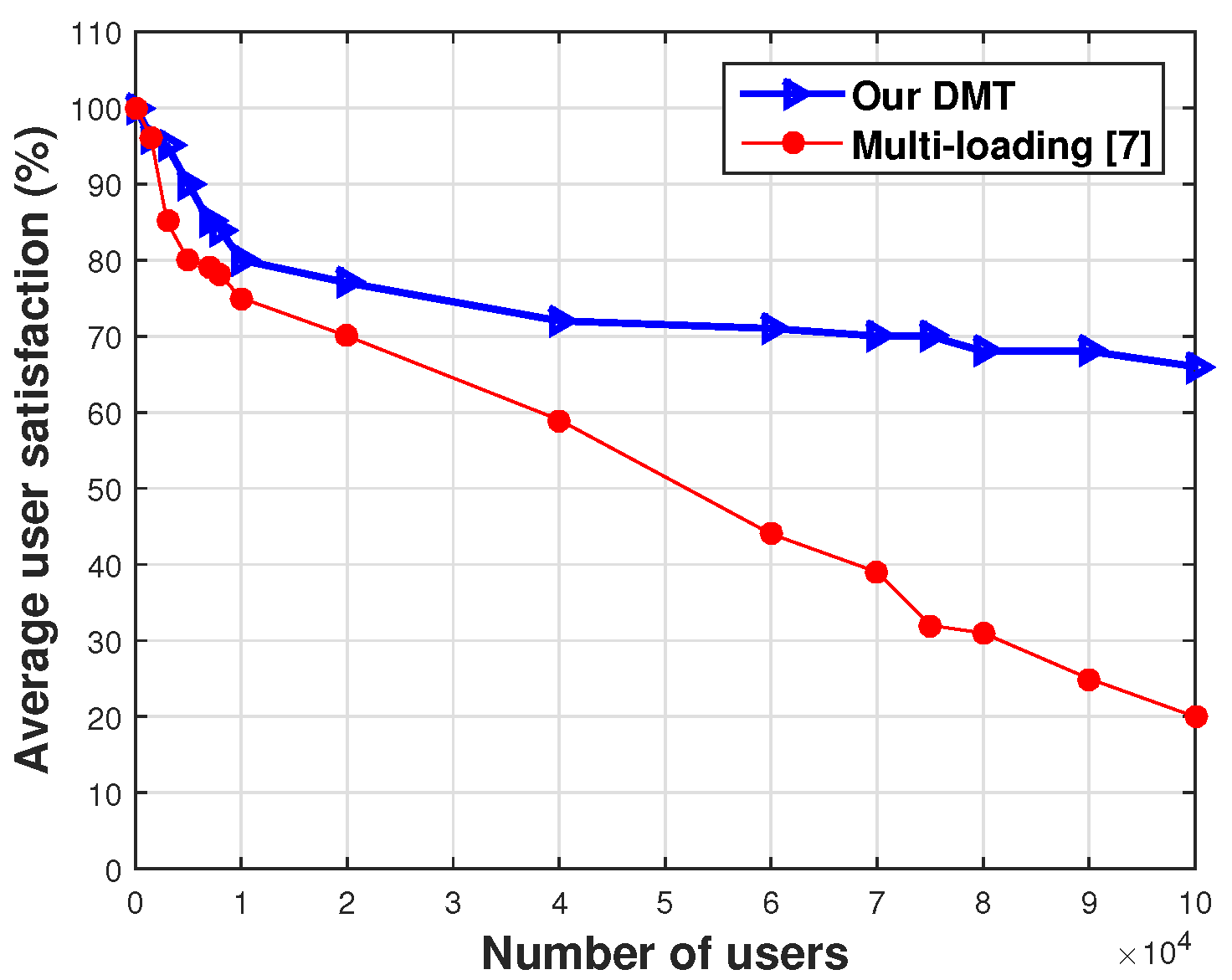
Figure 12 and Figure 13 compare the average user satisfaction for the DMT and a multi-loading algorithm for 40,000 and 100,000 passengers. We define user satisfaction as the number of passengers since the start of the trip divided by users who responded positively.

From Figure 12, we notice that the satisfaction rate of passengers using DMT or a multi-loading model decreases with increasing passenger density. The average user satisfaction when using DMT is higher than the average user satisfaction when using a multi-loading system.

It can be seen from

Table 9. Average user satisfaction savings rate in the case of using the DMT or the multi-load model.

Passenger Number Interval	DMT (%)	Multi-Load Model (%)	Saving Rate (%)
[1–40,000]	72	59	18.06
[40,001–60,000]	70	45	35.71
[60,001–100,000]	65	20	69.23

that the average user satisfaction when using DMT is higher than the average user satisfaction when using multi-loading. Similarly, the average satisfaction level does not change significantly as the number of passengers increases compared to that of the multi-load.

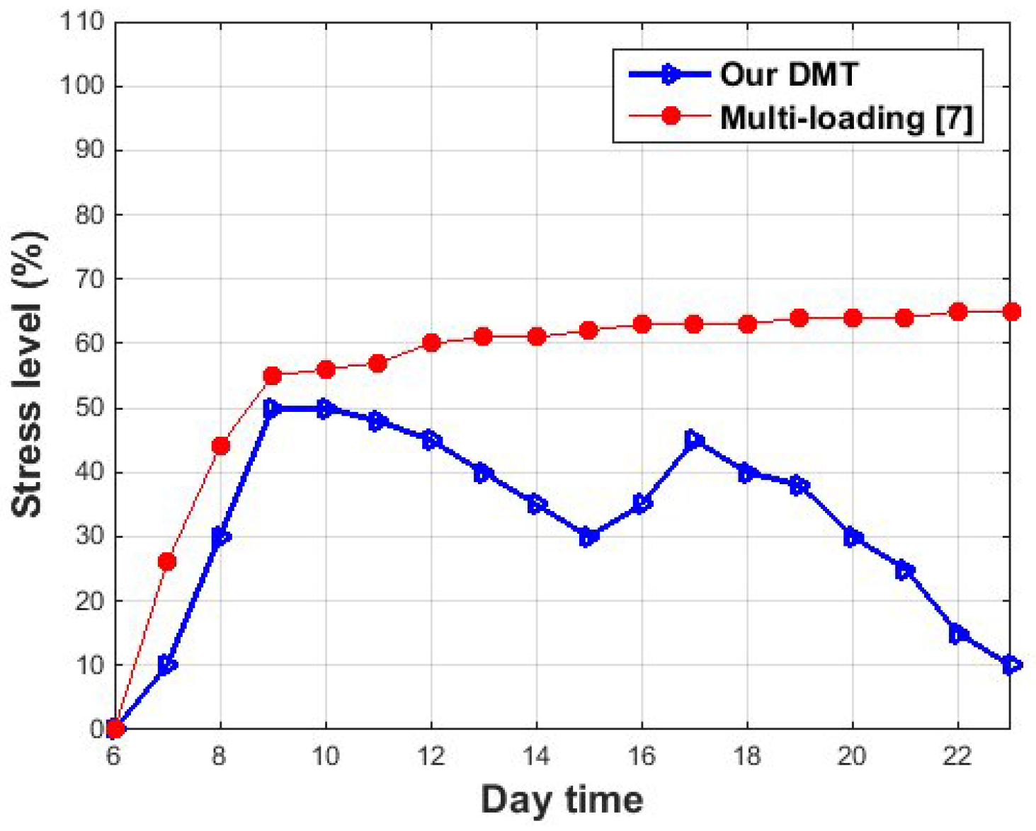
Figure 14 compares the stress level of passengers when using DMT and the multi-loading algorithm. For DMT and multi-load models, the proportion increased significantly in the morning period from 6 a.m. to 9 a.m., reaching approximately 50%. For DMT, the stress level decreases and increases during the day until 5 p.m. At 5 p.m., the stress level was 45%, after which the percentage decreased until it reached 10% at 11:00 p.m. In contrast, for the multi- loading model, the level increases smoothly and does not change significantly throughout the day.

From

Table 10. Average stress level saving rate in the case of using the DMT or the multi-load model.

Day Time	DMT (%)	Multi-Load Model (%)	Saving Rate (%)
[6:00 a.m.–9:00 a.m.]	50	55	9.09
[9:01 a.m.–3:00 p.m.]	30	62	51.61
[3:01 p.m.–5:00 p.m.]	45	63	28.57
[5:01 p.m.–12:00 p.m.]	10	65	84.61

, we found that the savings rate of average stress level between 6:00 a.m. and 9:00 a.m. was approximately 9.09% when using a multi-loading system. This ratio increased when the time reaches 3:00 p.m. At 3:00 p.m., the savings rate was around 28.57%. However, the maximum savings rate was reached at 11:59 p.m.: 84.61%.

Additionally, the error rate of delay time was estimated to be between 7% and 13% for all the three scenarios, as presented in Figure 13 and Table 9.

We can conclude that DMT provides superior performance than the multi-loading algorithm because it is based on measuring the satisfaction of individual passengers. Unlike the work of [7], DMT can dynamically and instantly update information about public buses, ride-sharing cars, and passengers.

We mention that in this work we did not use the location-based services (LBS) methods, but we acknowledge their importance in the smart city concept and especially in smart transportation. Indeed, in our system, (centralized/decentralized) LBS and their recommended applications can provide several smart services to users. For example, based on the collected and shared information, applications in LBS can enhance user experience through individuals’ reviews of users which build the reputation of a system and/or provide guidance/assistance through recommendations. Additionally, LBS could perform operation and maintenance issues for our multi-modal transportation system. However, as the LBS utilizes geographic data and passenger information, the privacy leaking and effectiveness of reviews is an important challenge.

6. Conclusions

In this paper, we developed a dynamic mobility traffic (DMT) model to enable passengers to use car ride-sharing and public buses together or one of them during their trip with the fastest time and lowest fare. At each station, passengers can be informed of the capacity of the car or public bus that will pass through the station, and the current position of each car or bus.

Practically, OMNET++, OpenStreetMap, and SUMO were used to implement DMT. Part of a map of the City of Ottawa was taken as a case study using OpenStreetMap. SUMO was used to create random movement on the streets, mainly including the traffic of public buses and cars. The results indicate that the average stress levels from the use of ride-sharing cars and public buses alone are similar. Those stress levels are higher than the stress level of using cars and buses in the optimal combination. In addition, the results highlight that passengers experience less satisfaction when using only public buses. Likewise, the satisfaction rate of passengers increases when using the appropriate combination of public buses and cars for transportation, thereby achieving lower cost and faster arrival.

Furthermore, DMT is compared with a multi-load model presented in [7]. The result of this comparison shows that our DMT is better in terms of lower fares and faster arrival times than a multi-load model.

The proposed model can be easily applied to cities other than Ottawa because the equations took into account the different traffic conditions and the different designs of roads within cities which are generated by a SUMO. Indeed, the model is suitable for short trips, not for long trips and a small city area. We plan to extend our DTM model for future works by considering more transportation forms, such as bicycles and trains. Additionally, electrified transportation can be an open issue for our DTM. We plan to study the privacy protection of our system regarding the LBS services, especially for the sake of reviews of users and for tracking transportation forms’ states.

References

- Muñoz-Villamizar, A.; Montoya-Torres, J.R.; Faulin, J. Impact of the use of electric vehicles in collaborative urban transport networks: A case study. Transp. Res. Part D Transp. Environ. 2017, 50, 40–54. [Google Scholar] [CrossRef]
- Ceccato, R.; Diana, M. Substitution and complementarity patterns between traditional transport means and car sharing: A person and trip level analysis. Transportation 2018, 1–18. [Google Scholar] [CrossRef]
- Barth, M.; Todd, M. Simulation model performance analysis of a multiple station shared vehicle system. Transp. Res. Part C Emerg. Technol. 1999, 7, 237–259. [Google Scholar] [CrossRef]
- Galland, S.; Knapen, L.; Yasar, A.U.H.; Gaud, N.; Janssens, D.; Lamotte, O.; Koukam, A.; Wets, G. Multi-agent simulation of individual mobility behavior in carpooling. Transp. Res. Part C Emerg. Technol. 2014, 45, 83–98. [Google Scholar] [CrossRef]
- Huang, H.; Bucher, D.; Kissling, J.; Weibel, R.; Raubal, M. Multimodal Route Planning with Public Transport and Carpooling. IEEE Trans. Intell. Transp. Syst. 2018, 20, 3513–3525. [Google Scholar] [CrossRef]
- Hariz, M.B.; Said, D.; Mouftah, H.T. Mobility traffic model based on combination of multiple transportation forms in the smart city. In Proceedings of the 2019 15th International Wireless Communications and Mobile Computing Conference (IWCMC), Tangier, Morocco, 24–28 June 2019; pp. 14–19. [Google Scholar]
- Miranda, D.M.; de Camargo, R.S.; Conceição, S.V.; Porto, M.F.; Nunes, N.T.R. A multi-loading school bus routing problem. Expert Syst. Appl. 2018, 101, 228–242. [Google Scholar] [CrossRef]
- Baggag, A.; Abbar, S.; Zanouda, T.; Srivastava, J. Resilience analytics: Coverage and robustness in multi-modal transportation networks. EPJ Data Sci. 2018, 7, 14. [Google Scholar] [CrossRef] [Green Version]
- Furuhata, M.; Dessouky, M.; Ordóñez, F.; Brunet, M.E.; Wang, X.; Koenig, S. Ridesharing: The state-of-the-art and future directions. Transp. Res. Part B Methodol. 2013, 57, 28–46. [Google Scholar] [CrossRef]
- Agatz, N.A.H.; Erera, A.L.; Savelsbergh, M.W.P.; Wang, X. Dynamic ride-sharing: A simulation study in metro Atlanta. Transp. Res. Part B Methodol. 2011, 45, 1450–1464. [Google Scholar] [CrossRef]
- Bast, H.; Delling, D.; Goldberg, A.; Müller-Hannemann, M.; Pajor, T.; Sanders, P.; Wagner, D.; Werneck, R.F. Route planning in transportation networks. In Lecture Notes in Computer Science; Springer: Berlin/Heidelberg, Germany, 2016; Volume 9220, pp. 19–80. [Google Scholar]
- Akiba, T.; Iwatat, Y.; Kawarabayashi, K.I.; Kawata, Y. Fast shortest-path distance queries on road networks by pruned highway labeling. In Proceedings of the Workshop on Algorithm Engineering and Experiments, Portland, OR, USA, 5 January 2014; pp. 147–154. [Google Scholar]
- Allulli, L.; Italiano, G.F.; Santaroni, F. Exploiting GPS data in public transport journey planners. In International Symposium on Experimental Algorithms; Springer: Berlin/Heidelberg, Germany, 2014; pp. 295–306. [Google Scholar] [CrossRef]
- Dibbelt, J.; Pajor, T.; Wagner, D. User-Constrained Multimodal Route Planning. J. Exp. Algorithmics 2015, 19, 1.1–1.19. [Google Scholar] [CrossRef] [Green Version]
- Pajor, T. Multi-Modal Route Planning. Universität Karlsruhe. 2009. Available online: https://i11www.iti.kit.edu/extra/publications/p-mmrp-09.pdf (accessed on 21 February 2021).
- Bucher, D.; Jonietz, D.; Raubal, M. A heuristic for multi-modal route planning. In Progress in Location-Based Services; Springer: Cham, Switzerland, 2016; pp. 211–229._11. [Google Scholar] [CrossRef]
- Massobrio, R.; Fagúndez, G.; Nesmachnow, S. Multiobjective evolutionary algorithms for the taxi sharing problem. Int. J. Metaheuristics 2016, 5, 67–90. [Google Scholar] [CrossRef]
- Zhu, M.; Liu, X.-Y.; Tang, F.; Qiu, M.; Shen, R.; Shu, W.; Wu, M.-Y. Public vehicles for future urban transportation. IEEE Trans. Intell. Transp. Syst. 2016, 17, 3344–3353. [Google Scholar] [CrossRef]
- Jung, J.; Jayakrishnan, R.; Park, J.Y. Dynamic shared-taxi dis- patch algorithm with hybrid-simulated annealing. Comput.-Aided Civil Infrastruct. Eng. 2016, 31, 275–291. [Google Scholar] [CrossRef]
- Aïvodji, U.M.; Gambs, S.; Huguet, M.J.; Killijian, M.O. Meeting points in ridesharing: A privacy-preserving approach. Transp. Res. Part C Emerg. Technol. 2016, 72, 239–253. [Google Scholar] [CrossRef] [Green Version]
- Czioska, P.; Trifunović, A.; Dennisen, S.; Sester, M. Location- and time-dependent meeting point recommendations for shared interurban rides. J. Locat. Based Serv. 2017, 11, 181–203. [Google Scholar] [CrossRef] [Green Version]
- Zhu, M.; Liu, X.Y.; Wang, X. An Online Ride-Sharing Path-Planning Strategy for Public Vehicle Systems. IEEE Trans. Intell. Transp. Syst. 2019, 20, 616–627. [Google Scholar] [CrossRef]
- Aissat, K.; Varone, S. Carpooling as complement to multi-modal transportation. In International Conference on Enterprise Information Systems; Springer: Berlin/Heidelberg, Germany, 2015; pp. 236–255. [Google Scholar]
- Varone, S.; Aissat, K. Multi-modal transportation with public transport and ride-sharing: Multi-modal transportation using a path-based method. In Proceedings of the 17th International Conference on Enterprise Information Systems, Barcelona, Spain, 27–30 April 2015. [Google Scholar]
- Pi, X.; Ma, W.; Qian, Z. A general formulation for multi-modal dynamic traffic assignment considering multi-class vehicles. Transp. Res. Part Emerg. Technol. 2019, 104, 369–389. [Google Scholar] [CrossRef]
- Dimokas, N.; Kalogirou, K.; Spanidis, P.; Kehagias, D. A mobile application for multimodal trip planning. In Proceedings of the 2018 9th International Conference on Information, Intelligence, Systems and Applications (IISA), Zakynthos, Greece, 23–25 July 2018; pp. 1–8. [Google Scholar]
- Cangialosi, E.; Di Febbraro, A.; Sacco, N. Designing a multimodal generalised ride sharing system. IET Intell. Transp. Syst. 2016, 10, 227–236. [Google Scholar] [CrossRef]
Figure 1.
A dynamic mobility traffic model overview.
Figure 2.
A time-expanded diagram of a public bus network.
Figure 3.
A time-expanded diagram of a car ride-sharing network.
Figure 4.
The data exchanged between the regional manager, the public buses, the ride-sharing cars and the riders.
Figure 5.
The interactions between a user and the DMT model.
Figure 6.
Case study: a map of Ottawa.
Figure 7.
An example of a passenger’s route from his origin to his destination.
Figure 8.
The average user satisfaction.
Figure 9.
The average transportation stress level.
Figure 10.
The inputs and the outputs of the multi-load.
Figure 11.
The inputs and the outputs of the DMT model.
Figure 12.
Average user satisfaction for the DTM and the multi-load model when the number of users is 40,000.
Figure 13.
Average user satisfaction for the DMT and the multi-load model when the number of users is 100,000.
Figure 14.
Average stress level for the DMT and the multi-load model when the number of users is 24,000.