Article

Interdependencies of Infrastructure Investment Decisions in Multi-Energy Systems—A Sensitivity Analysis for Urban Residential Areas

1
Grid Planning and Operation Division, Fraunhofer Institute for Energy Economics and Energy System Technology, 34119 Kassel, Germany
2
Grid Planning Department, Stadtwerke Bamberg Energy and Water Supply Company, 96052 Bamberg, Germany
3
Faculty of Electrical Engineering and Computer Science, University of Applied Science Coburg, 96450 Coburg, Germany
4
Department of Energy Management and Power System Operation, University of Kassel, 34119 Kassel, Germany
*
Author to whom correspondence should be addressed.
Submission received: 9 December 2020 / Revised: 28 December 2020 / Accepted: 5 January 2021 / Published: 8 January 2021
(This article belongs to the Special Issue Innovative Energy Systems for Smart Cities)

Abstract

:
Considering the European Union (EU) climate targets, the heating sector should be decarbonized by 80% to 95% up to 2050. Thus, the macro-trends forecast increasing energy efficiency and focus on the use of renewable gas or the electrification of heat generation. This has implications for the business models of urban electricity and in particular natural gas distribution network operators (DNOs): When the energy demand decreases, a disproportionately long grid is operated, which can cause a rise of grid charges and thus the gas price. This creates a situation in which a self-reinforcing feedback loop starts, which increases the risk of gas grid defection. We present a mixed integer linear optimization model to analyze the interdependencies between the electricity and gas DNOs’ and the building owners’ investment decisions during the transformation path. The results of the investigation in a real grid area are used to validate the simulation setup of a sensitivity analysis of 27 types of building collectives and five grid topologies, which provides a systematic insight into the interrelated system. Therefore, it is possible to identify building and grid configurations that increase the risk of a complete gas grid shutdown and those that should be operated as a flexibility option in a future renewable energy system.

1. Introduction

The heat sector accounts for about 48% of the global final energy, 27% of which comes from renewable sources [1]. Among the remaining 73% of fossil fuels, natural gas plays an important role. In the European Union (EU), heating and cooling applications account for about 50% of final energy demand, of which 42% are gas-fired and 12% are electricity-based systems [2]. Based on current EU targets, the heat sector should be decarbonized by 80–95% by 2050 compared to 1990 [1,2].
According to current studies, two macro-trends can be identified: On the one side, primarily gas-based systems fired with CO2 neutral gases and carbon capture technologies are used to mitigate emissions, as suggested by Irish, British [3,4,5], Chinese [6,7], and US [8,9,10,11] studies. On the other side, a strong electrification of the heat generation is predicted. In this scenario, gas-fired systems are mostly substituted by electrical heat pumps. According to German studies, this could reduce the gas demand by 25–100% in 2050 [12,13,14,15].
In both scenarios, the studies assume that the transformation path is strongly steered by national CO2-related political and regulatory instruments. On the one hand, this triggers a technological change in heat generation, as fossil-fired heating systems such as gas burners are substituted by more efficient systems such as electric heat pumps. On the other hand, an increase in energy efficiency is triggered, which further enhances the attractiveness of heat pumps. Both aspects lead to a decline in gas demand [14]. As heat applications account for 61% of the gas demand on average for all 28 EU countries [2], energy efficiency improvements or a substitution of gas-based systems have a strong effect on the gas network operator’s supply task and thus on its future business model. An economic risk will arise for the gas distribution network operators (DNOs) in the future: If energy efficiency rises and the number of gas customers drops, a disproportionately long gas network has to be operated for a decreasing amount of energy, which—depending on the DNO strategy and regulatory environment—leads to a decrease in the profitability of the grid and finally to an increase in grid charges [16,17] (Figure 1).
Furthermore, this could pose a risk to the continued existence of the entire natural gas infrastructure: By looking at heating retrofit measures in building stock at present, electric heat pumps are economically less attractive than fossil-fired systems due to their high power-specific investment expenditures [19] and requirements regarding heating circuit temperatures [20]. Often, they are installed because of legal requirements and subsidies, or in energy-efficient new or retrofitted buildings [21]. A rise in grid charges leads to an increase in operating expenses for gas-fired heating systems, which makes a replacement of the heating or building surface insulation measures economically more attractive to the building owner. Due to the high sensitivity of the operational expenses of gas heating systems to energy price fluctuations, it is possible that with a rising gas price, price parity of operational (OPEX) and investment expenditures (CAPEX) between gas burners and electric heat pumps will be achieved in the future. The point where a self-reinforcing feedback loop starts could trigger the defection of the gas grid [22]. This represents an endogenous feedback effect within the interrelated system of the gas and electricity DNO and building owners that mostly has been neglected in energy system analysis so far.
The proposed feedback effect is especially pronounced when looking at urban residential areas: As the profitability of gas grids rises with the load density [17], they are predominantly operated in densely populated rural or urban areas with a high connection rate of the buildings to the gas grid. Where heating networks can be constructed and operated economically in commercial and mixed areas with high energy consumption, their new construction is often uneconomic in residential building stock with an existing gas grid. In this case, gas burners are frequently replaced by electric heat pumps [12,14,23].
Most energy system, building retrofit, or grid planning studies neglect the proposed business dynamics: On the one side, investigations concerning the future transformation paths of the building stock, which are usually based on models for the optimization of energy-efficient building design, are in use. The optimization goals are the minimization of the energy consumption, CO2 emissions, or cost and comfort issues in single buildings or the building stock [24], where they analyze how the technological development is steered by technological and market trends or regulatory and political instruments such as CO2 pricing, energy efficiency requirements, or technology promotion [5,9,13,25]. Electricity and natural gas grid charges are predetermined exogenous variables, while interactions between individual actors and the circumstances at the local grid level are neglected.
On the other side, most natural gas and electricity grid planning approaches, especially at the distribution grid level, focus on restructuring, grid reinforcement, or the integration of renewable feed-ins [26,27,28,29]. The supply task—the position and behavior of a load or generator—is a predefined exogenous input variable [30].
There are studies that investigate the interactions between investment decisions in buildings and investment decisions of the grid operator in the electricity sector mostly with the focus on self-supply [31,32,33,34]. Work exists that has transferred these approaches to the gas sector: Some focus on the development of the gas DNO’s business model and the corresponding grid charge development [16,17]. Others examine the feedback effect between actors in a specific network area and analyze the impact of variations in the regulatory and political framework and DNO strategies [22].
There is a lack of work evaluating the influence of building and grid-specific parameters on the investment decisions of the individual actors, the interaction between them, and the consequences for the transformation path. In our analysis, we focus on the evaluation of the influence of building- and network-specific parameters on the feedback effect between the gas and electricity DNO grid charge setting and building retrofit decisions in densely populated rural or urban residential areas. Thereby, we address three questions that are relevant for DNOs, policy makers, and energy economists:
  • What are the building-, heating-, and grid-specific factors that influence significant changes in the energy supply infrastructure, such as gas grid defection?
  • How are these building-, heating-, and grid-specific influencing factors pronounced in real urban grid areas?
  • How are the endogenous variables (gas demand, gas grid charges) shaped within the transformation path and influenced by different configurations of the exogenous variables (building type and age, heating system configuration, grid topology)?
  • Which configuration of exogenous factors (building type and age, heating system configuration, grid topology) results in an equilibrium between the construction and replacement of gas-based heating systems, fosters gas-based systems, or leads to the collapse of the gas grid infrastructure?
To answer the questions, we present a mixed integer linear program (MILP) (Section 2.1 and Section 2.4). We model the building stock, consisting of the individual single buildings that want to minimize their total costs for heating by renovation (Section 2.2). We model an electricity DNO and a gas DNO (Section 2.3), which define their investment strategy based on the building owners’ investment decisions in order to keep the reliability at the initial level. We determine the key influencing factors on the basis of a meta-analysis (Section 3.1) and examine their characteristics in the area of the southern German city of Bamberg (Section 3.2). To analyze the interdependencies and influencing factors during the transformation, a case study on a selected real grid area is performed (Section 3.3). This grid area has already been analyzed on the basis of a multi-agent analysis in which the authors use the same building retrofit model [22]. This detailed analysis of the real grid area allows us to validate our simplified grid and DNO model. We use this validated model to perform a sensitivity analysis of 27 types of building collectives and five gas grid topologies (Section 3.4). The results of the structural grid analysis of Section 3.3 are used to define the simulation setup. In the final step, we discuss the conclusions (Section 4).

2. Materials and Methods

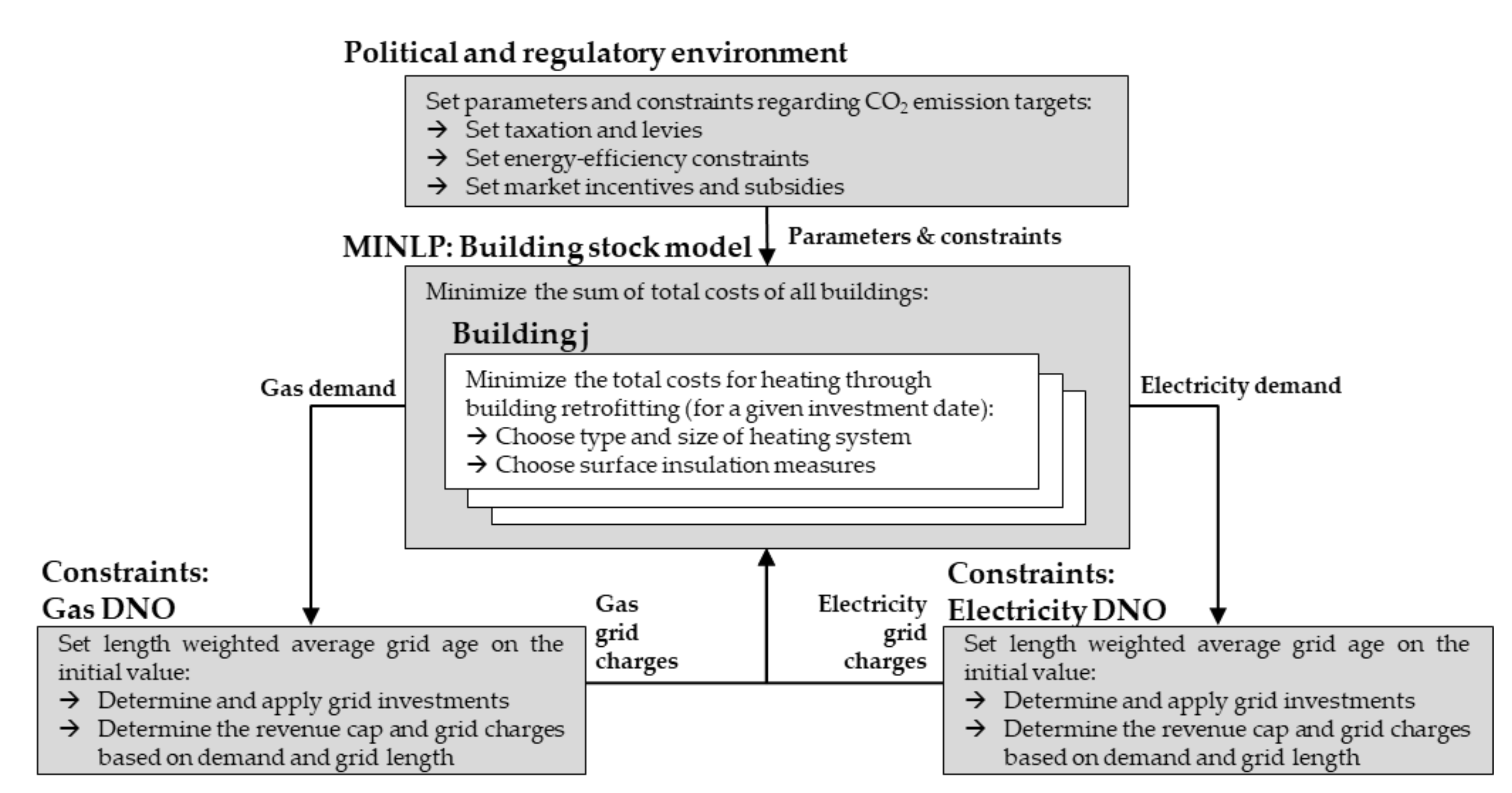
2.1. Research Approach

We are focusing on the investigation of the feedback effects of the grid charge increase on the building retrofit decisions. For that reason, we introduce a linearized mixed integer nonlinear program (MINLP): The optimization problem is to minimize the total cost of heating in all buildings in an area by retrofitting the heating system and the building surface. This optimization problem is constrained by the electricity and gas DNO’s strategic decisions. The respective DNO renews and maintains the grid in order to maintain supply reliability. In this way, it adjusts the grid charges depending on the supplied energy, network length, and grid investments to keep the grid age at the initial level to guarantee a stable supply. The other way around, the retrofit decisions fix the demand of electricity and gas as well as the corresponding grid length (Figure 2).
The interrelated system of building owners and distribution network operators represents a conflicting situation, due to the opposing objectives of the actors. In a collapsing monopoly, as it is proposed for the gas grid, it corresponds to a hierarchically structured bi-level problem. The building owners’ decisions in the upper level are constrained by the DNO optimization problems in the lower level. Both problems are connected through an equilibrium in volume and price, which is related to Stackelberg games in microeconomics [35]: The sum of the buildings represents the leader, which anticipates the energy price for one year, optimizes its strategy accordingly, and fixes the amount of supplied energy. The DNO represents the follower, which adjusts the grid charges for the transportation service in order to clear the market for the transported energy. If the lower level problem is linear, it can be integrated in the upper level by replacing it with its primal and dual constraints as well as the strong duality theorem, by modeling a mathematical program with primal and dual constraints (MPPDC) [31,34,36].
In our case, the supply task, i.e., the required grid length and the energy supplied, is determined by the decisions of the building owners. For the chosen strategy, the DNO can achieve its target—to keep the length weighted grid age at the initial level—for all time steps independent of the building owner’s decision (as long as the grid exists). Due to this non-conflicting situation, the bi-level is reduced to a single-level approach [36]: The length weighted grid age is set to the initial level for the planning horizon and the DNO problem is replaced by its central equality constraint—cost equals revenue—in order to integrate it into the building optimization problem.

2.2. Building Energy Retrofit Model

2.2.1. Optimization Problem

The building owners want to minimize their total costs for heating. To reach this goal, they perform one building and heating system retrofit during the planning horizon from 2020 to 2050. The date of investment of each building is a predefined exogenous variable. On this date, the building owner must renew or change the heating system and has the opportunity to reinforce the building insulation, install a solar thermal system (STE), and lower the heating circuit temperature.
All cost components and technical parameters of the building equipment options required for a respective heating system, such as a chimney, a fuel store, or a hot water tank, are calculated individually for each building or heating in a preprocessing procedure. We consider the whole building stock of a grid area by minimizing the sum of the total costs of the individual buildings. The optimization model for a single building and the corresponding parameters used were introduced in [22]. A simplified version of the model is shown in this paper to explain the basic relationships; for the detailed sub models that are listed in Appendix B, see [22]. For a list of the acronyms used, see Table A1 and Table A2 in Appendix A.

2.2.2. Objective Function

The objective is to minimize of the sum of the total costs of all buildings 𝒥 that perform a retrofit in the year 𝓉 of the planning horizon T P l a n n i n g (Equation (1)).
min c B = 𝒿 J c 𝒿 B
Within the retrofit decision of a single building 𝒿, we consider the capital expenditure (CAPEX) for a change of the heating system c 𝒿 BES , the improvement of the building surface c 𝒿 BE , the operational expenditure (OPEX) for maintenance c 𝒿 M , and energy procurement c 𝒿 EN (Equation (2)). The OPEX is calculated for the technical lifetime of the heating system of 33.5 years, which is based on annual time steps. The calculation interest rate for the building owners is set to 0% for c 𝒿 M , respectively 4% for c 𝒿 EN .
𝒿 J :   c 𝒿 B = c 𝒿 BE + c 𝒿 BES + c 𝒿 EN + c 𝒿 M
  • c 𝒿 BE : The investment expenditure for the building envelope retrofit c 𝒿 BE (Equation (3)) is a function of the insulation thickness D 𝒹 D and the building surface area A 𝒿 E , which is calculated based on the different surface parts 𝓅 [22]. The building surface is modeled in a single zone. The design-relevant heat load S 𝒹 , 𝒿 BE is calculated based on DIN EN 12,831 (German and European harmonized standard) [37]. The optimizer can choose an additional insulation between 0 and 30 cm. The cost parameters C 𝒿 BEfix and C 𝒿 BEvar are calculated individually for every building based on the area ratios of the individual surface parts A 𝒿 , 𝓅 EP and the corresponding costs [38]: roof, facade, windows, floor, and door.
    c 𝒿 BE =   𝒹 D A 𝒿 E C 𝒿 BEvar D 𝒹 D + C 𝒿 BEfix b 𝒹 , 𝒿 B E ; w i t h   A 𝒿 E = 𝓅 P 𝒿 A 𝒿 , 𝓅 EP ; C 𝒿 BEfix = 𝓅 P C 𝒿 , 𝓅 BEfix A 𝒿 , 𝓅 EP A 𝒿 E ;   C 𝒿 BEvar = 𝓅 P C 𝒿 , 𝓅 BEvar A 𝒿 , 𝓅 EP A 𝒿 E
  • c 𝒿 BES : The investment expenditure for the building energy system c 𝒿 BES (Equation (4)) is a function of the building heat load S 𝒹 , 𝒿 BE and the size of the solar thermal plant S 𝓈 , 𝒿 STE [22]. S 𝒹 , 𝒿 BE represents the design-relevant heat load [37], including transmission and ventilation losses. The available heating systems are an air water heat pump (AWHP), a gas condensing boiler (GCB), an oil condensing boiler (OCB), a pellet burner (PB), and an electrical direct heating (EDH). C 𝓀 BESvar and C 𝓀 ,   𝒿 BESfix are the corresponding specific cost parameters. Additionally, the optimizer is able to install a solar thermal system (STE) and lower the heating circuit temperature to increase the efficiency. C 𝓈   STEvar and C 𝓈 , 𝒿   STEfix are the corresponding specific cost parameters (STE).
    c 𝒿 BES =   𝓀 K 𝒹 D S 𝒹 , 𝒿 BE b 𝒹 , 𝒿 B E C 𝓀 BESvar + C 𝓀 ,   𝒿 BESfix b 𝓀 ,   𝒿 B E S + 𝓈 S S 𝓈 , 𝒿 STE C 𝓈   STEvar + C 𝓈 , 𝒿   STEfix b 𝓈 , 𝒿 S T E
  • c 𝒿 EN : The expenditure for energy procurement c 𝒿 EN (Equation (5)) is a function of the building heat load S 𝒹 , 𝒿 BE , the domestic hot water demand S 𝒿 DHW , the size of the solar thermal plant S 𝓈 , 𝒿 STE , and the additional wins and losses S 𝒿 S , as well as the plant expenditure figure E 𝓀 BES , the yearly usage hours T 𝒿 N , the costs for energy procurement in the year of investment C 𝒸 , 𝓉 = 𝓉 I n v e s t EC , and the present value factor for energy procurement PF EN [22]. The additional heat losses and wins S 𝒿 S include heat distribution losses, auxiliary energy, radiation losses, and internal wins [39,40]. They are not affected by the retrofit. The specific cost parameter C 𝒸 , 𝓉 = 𝓉 I n v e s t EC is calculated based on the energy procurement price C 𝒸 , 𝓉 Proc , tax C 𝒸 , 𝓉 Tax , and grid charges c 𝒸 , 𝓉 = 𝓉 I n v e s t GC .
    c 𝒿 EN =   𝓀 K 𝒹 D S 𝒹 , 𝒿 BE b 𝒹 , 𝒿 B E +   S 𝒿 S b k ,   𝒿 B E S + 𝓈 S S 𝒿 DHW S 𝓈 , 𝒿   STE b 𝓈 , 𝒿 S T E b 𝓀 , 𝒿 B E S T 𝒿 N E 𝓀 BES 𝒸 C B 𝒸 , 𝓀 EC C 𝒸 , 𝓉 = 𝓉 I n v e s t EC PF EN w i t h   C 𝒸 , 𝓉 = 𝓉 I n v e s t EC = C 𝒸 , 𝓉 = 𝓉 I n v e s t Proc +   C 𝒸 , 𝓉 = 𝓉 I n v e s t Tax   + c 𝒸 , 𝓉 = 𝓉 I n v e s t G C ,     | f o r   c = electricity c = gas C 𝒸 , 𝓉 = 𝓉 I n v e s t Proc +   C 𝒸 , 𝓉 = 𝓉 I n v e s t Tax                         ,     | f o r   c = pellet c = oil
  • c 𝒿 M : The operation expenditure for the maintenance of the building energy system c 𝒿 M (Equation (6)) is determined based on a fixed yearly rate M 𝓀 BES dependent on the heating system and solar thermal plant type and size ( S 𝒹 , 𝒿 BE and S 𝓈 , 𝒿 STE ), as well as the present value factor for maintenance PF M [22].
    c 𝒿 M   = 𝓀 K 𝒹 D S 𝒹 , 𝒿 BE b 𝒹 , 𝒿 B E C 𝓀 BESvar + C 𝓀 , 𝒿 BESMfix b 𝓀 , 𝒿 B E S M 𝓀 BES PF M + 𝓈 S S 𝓈 , 𝒿 STE C 𝓈   STEvar + C 𝓈 , 𝒿   STEfix M 𝓈 STE b 𝓈 , 𝒿 S T E PF M

2.2.3. Constraints and Parameter Setting

We constrain the number of measures for one building considering the heating, the solar thermal plant, and the building surface. The optimizer:
  • Can choose a building surface insulation measure,
  • Has to replace the heating system, and
  • Can choose a solar thermal plant.
Additionally, we set the parameters and add constraints, corresponding to the situation in Germany [22]:
  • Regulatory energy efficiency constraint: We limit the yearly CO2 emissions and the final energy demand to an upper bound of the initial demand Q 𝒿 H init . Additionally, we constrain the yearly primary energy demand to Q 𝒿 P EnEV , which is a demand that is calculated based on the energy-efficiency targets of the energy-saving ordinance of Germany [41].
  • Retrofit rate of building envelope and heating system: The literature covers renovation rates of about 3.3% for heating systems and about 2–3% for building envelope retrofits. This corresponds to a technical lifetime of the heating system of about 30 years and of the surface of about 40–50 years [42]. We set the date of investment of each building in order to reach this heating retrofit rate (approximately 3%). Additionally, we oblige 66% of buildings to retrofit their envelope and heating system; this corresponds to an envelope retrofit ratio of approximately 2%.
  • Taxation and levy systems: We calculate the levies and taxes with regard to the current energy prices in Germany and grid charges in the city area of Bamberg. In addition, we use a CO2 price, which will increase from 25 €/t in 2019 to 65 €/t in 2026 [43].
  • Grid charge models: We reduce the electricity grid charges for heat pumps and electrical heatings down to 25% of their regular value, due to the German law [44].
  • State market incentive and subsidy programs: We reduce the specific expenditure for building envelope retrofits about 30%, considering a state subsidy program in Germany [45]. For heat pumps, there is a market incentive program [46], so we add a subsidy rate of 40%.

2.3. Distribution Network Operator Model

2.3.1. Supply Task: Relationship between Energy Supplied, Customer Number, and Grid Length

The DNO’s revenues depends not only on the cost allocation between CAPEX and OPEX but also on the energy supplied as well as the grid length and age [17,22]. Where the energy demand is directly dependent on user behavior and the building owners’ investment decisions, the length depends indirectly on these decisions: The location and size of grid users—the so-called supply task—determines the grid length [16]. In this way, from the DNO’s point of view, the grid length, energy supplied, and customer number are exogenous variables that are determined by the building owners’ decisions. We use an abstract model based on a power function to estimate the dependency between grid length l 𝒸 ,   𝓉   Grid and customer number n 𝓉 Cust in the grid and model all assets of the grid in a joint way. This approach is based on graph-theoretical considerations [47] and [16] (Equation (7)).
𝓉 T , 𝒸 :   l 𝒸 ,   𝓉   Grid =   l 𝒸   Gridmax * n 𝒸 , 𝓉 Cust n 𝒸 Gridmax k
We use Equation (7) to determine the relationship between the customer number in the grid n 𝒸 , 𝓉 Cust and the grid length l 𝒸 , 𝓉 Grid for an energy carrier 𝒸 (electricity or gas) and a time step 𝓉. In this context, n 𝒸 Gridmax represents the customer number when every building is connected to the grid and l 𝒸   Gridmax is the corresponding grid length. The exponent k is a measure of the disorder of the network [47,48,49,50]. It describes the non-linearity between grid length and customer number. Other work [16] has determined typical values for k in 57 real grids in the range of 0.4 to 0.5 for randomized exits with a high fit quality (R2 > 0.9). This is consistent with the predictions of network theory, where the values range from 1.0 for ordered networks to 0.33 for maximal disordered networks [47]. In the optimization model, we linearize the power function via a linear piecewise formulation [51]. Four grid points are set, whereby their positions are estimated with a least-square-fit [52].
The energy supplied in electricity distribution grids e 𝒸 ,   𝓉 Grid is not only determined by heating applications e 𝒸 , 𝓉 Heating . There are also other demands E 𝒸 , 𝓉 AnyOther (exogenous parameter), which are not affected by building retrofits (Equation (8)). This means that over the entire planning horizon, all buildings are connected to the electricity grid—independent their retrofit decision. As a result, the grid length remains at the initial value. In the residential areas under investigation, the entire gas demand is responsible for heating applications, so the number of customers varies with the building investment decision.
𝓉 T , 𝒸 :   e 𝒸 , 𝓉 Grid =   e 𝒸 , 𝓉 Heating +   E 𝒸 , 𝓉 AnyOther

2.3.2. Distribution Network Operator’s Investment Decisions

In the EU, gas and electricity supply are vertically unbundled. The grid infrastructure itself is subject to a natural monopoly; therefore, it is regulated to ensure stable supply quality and efficiency [17,22]. As the regulatory regime differs from country to country [53], we use a basic approach corresponding to the revenue-cap regulation currently applied in most European countries, especially in Germany [53]. Thereby, the grid charges are determined on the basis of the marginal costs for grid operation plus a return on equity determined by the regulator [16,54]: The annual 𝓉 operational α 𝒸 , 𝓉 OPEX (OPEX) and capital expenditures α 𝒸 , 𝓉 CAPEX (CAPEX) are added up for each energy carrier 𝒸 and passed on to grid customers in form of energy-based grid charges c 𝒸 , 𝓉 GC , depending on the energy supplied for heating e 𝒸 , 𝓉 Heating and other demands E 𝒸 , 𝓉 AnyOther ; see Equation (9). For a list of the acronyms used, see Table A3 in Appendix A.
  𝓉 T , 𝒸 :   α 𝒸 , 𝓉 CAPEX + α 𝒸 , 𝓉 OPEX   c 𝒸 , 𝓉 GC e 𝒸 , 𝓉 Heating + E 𝒸 , 𝓉 AnyOther = 0
We model all components of CAPEX and OPEX corresponding to [16,17,22]: The CAPEX is divided into interest on equity α 𝒸 , 𝓉 EC and borrowed capital α 𝒸 , 𝓉 BC , trade tax α 𝒸 , 𝓉 Tax , and the depreciations α 𝒸 , 𝓉 Depr . They are modeled dependent on the grid length l 𝒸 , 𝓉 Grid , age, and the corresponding technical lifetime (based on the normalized mean rest book value of all assets mrbvf 𝒸 , 𝓉 ). The OPEX is divided into other operational costs α 𝒸 , 𝓉 OC , which are modeled dependent on the grid length as well as loss costs α 𝒸 , 𝓉 LC , upstream grid charges α 𝒸 , 𝓉 UpGC , and concession fees α 𝒸 , 𝓉 Conc , which are modeled dependent on the energy supplied e 𝒸 , 𝓉 Grid (Table 1).
The literature provides several models for the analysis of the DNO’s cash flow; some of them consider each grid asset [22], others analyze the asset base in a cumulated model [16,17,34]. We use a simplified model according to [16], where we compare the results for a real grid with [22] to validate the results. In this way, we do not model the individual grid assets. The grid is represented by its length l 𝒸 , 𝓉 Grid and the corresponding age A 𝒸 , Grid rather than the cumulated rest book value RBV 𝒸 , 𝓉 Grid of all fixed assets, which is represented by the mean rest book value factor. RBV 𝒸 , 𝓉 Grid is calculated based on the length-specific historical investment expenditures C 𝒸 Grid , the grid length l 𝒸 , 𝓉 Grid and the average residual book value factor mrbvf 𝒸 , 𝓉 according to Equation (10).
  𝓉 T , 𝒸 :   RBV 𝒸 , 𝓉 Grid =   C 𝒸 Grid   ·   l 𝒸 , 𝓉 Grid   ·   mrbvf 𝒸 , 𝓉
The initial average rest book value factor is calculated depending on the technical life T   TL and the length-weighted average grid age that is dependent on the length L 𝒸 , l and age T   Init of each line (Equation (11)).
  𝒸   ϵ   C :   mrbvf 𝒸 , 𝓉 = 0 = 1 L L 𝒸 , l · T   Init L 𝒸 , 𝓉 T   TL
Equation (12) shows exemplarily how the interest on equity α 𝒸 , 𝓉 EC is calculated for the whole grid based on the equity interest rate R 𝒸 BC and the equity ratio Q 𝒸 BC :
  𝓉 T , 𝒸 :   α 𝒸 , 𝓉 EC =   R 𝒸 BC   ·   Q 𝒸 BC   ·   C 𝒸 Grid   ·   l 𝒸 , 𝓉   Grid   ·   mrbvf 𝒸 , 𝓉 .
Depending on the scenario—for a rising or falling demand—and the respective design of the regulatory regime—from cost-based to price-based to revenue-based approaches—different objectives for the DNO are desirable [22,55]. The goal of a DNO with a tendency of a decreasing demand is to maintain its business model as long as possible. In this way, it tries to maintain the set target value at a constant initial level during the planning horizon [17,54]: While fixing the revenue cap to the initial level (corresponding to cost-based or revenue-based approaches) leads to an increase in the quality of supply and a decline in supply efficiency, the opposite effect occurs when fixing the grid charges (corresponding to price-based approaches). For increasing demand, both effects are reversed. We use an approach where the DNO keeps its grid age, which is represented by the mean rest book value factor mrbvf 𝒸 , 𝓉 , on the starting level to ensure a constant quality of supply, independent of the demand scenario [55] (Equation (13)).
  𝓉 T , 𝒸 :   mrbvf 𝒸 , 𝓉 =   mrbvf 𝒸 , 𝓉 = 0

2.3.3. Integration of the DNO into the Building Model

Both the electricity and gas DNO set their investment ratios in order to keep the average asset age of the grid at the initial level. For this purpose, the variable mrbvf 𝒸 , 𝓉 is set to the initial level for each year in the planning horizon. As a consequence, the original optimization problem can be replaced by a central equality constraint—according to the basic relationship of Equation (9)—and integrated into the building model; see Equation (14). The components of the revenue cap are split into CAPEX and OPEX.
  𝓉 T , 𝒸 : R 𝒸 BC · Q 𝒸 BC + R 𝒸 Tax + 1 · R 𝒸 EC · Q 𝒸 EC + 1 T 𝒸 TL · C 𝒸 I · l 𝒸 ,   𝓉   Grid · mrbvf 𝒸 , 𝓉 = 0   + l 𝒸 , 𝓉 Grid · C 𝒸 LRC + C 𝒸 UpGC + C 𝒸 Conc + C 𝒸 LC · F 𝒸 Loss · e 𝒸 , 𝓉 Heating +   E 𝒸 , 𝓉 AnyOther   c 𝒸 , 𝓉 GC e 𝒸 , 𝓉 Heating +   E 𝒸 , 𝓉 AnyOther = 0
Corresponding to [16,17], the components of the CAPEX depend on the grid length l 𝒸 , 𝓉 Grid in year 𝓉, the historical acquisition costs C 𝒸 I , and the mean rest book value factor mrbvf 𝒸 , 𝓉 , which is set to its initial value 𝓉 = 0: The return on equity α 𝒸 , 𝓉 EC is a function of the equity ratio Q 𝒸 EC and interest rate R 𝒸 EC . The interests on borrowed capital α 𝒸 , 𝓉 BC are dependent of the debt ratio Q 𝒸 BC and interest rate R 𝒸 BC . The trade tax α 𝒸 , 𝓉 Tax is a part of the return on equity, which is calculated based on R Tax . The depreciations α 𝒸 , 𝓉 Depr are dependent of the reciprocal technical lifetime of the grid assets T 𝒸 TL . The OPEX consists of the other operational costs α 𝒸 , 𝓉 OC , which are dependent on the grid length as well as the upstream grid charges α 𝒸 , 𝓉 UpGC , the loss costs α 𝒸 , 𝓉 LC , and the concession fees α 𝒸 , 𝓉 Conc , depending on the respective specific costs C 𝒸 UpGC , C 𝒸 LC , C 𝒸 Conc , and losses F 𝒸 Loss , as well as the energy supplied. Additional constraints are necessary for linearization and the mapping of the problem to the situation in Germany:
  • Upper and lower limits for the grid charges: The grid charges are limited downwards (0 €) as well as upwards (100 €).
  • Constraints due to the linearization of products of continues variables ( c 𝒸 , 𝓉 GC   e 𝒸 , 𝓉 Heating ) : To linearize these products of two continuous variables, we discretize the energy [31] and substitute the resulting product of a binary and continuous variable via an additional variable and four constraints considering [51].

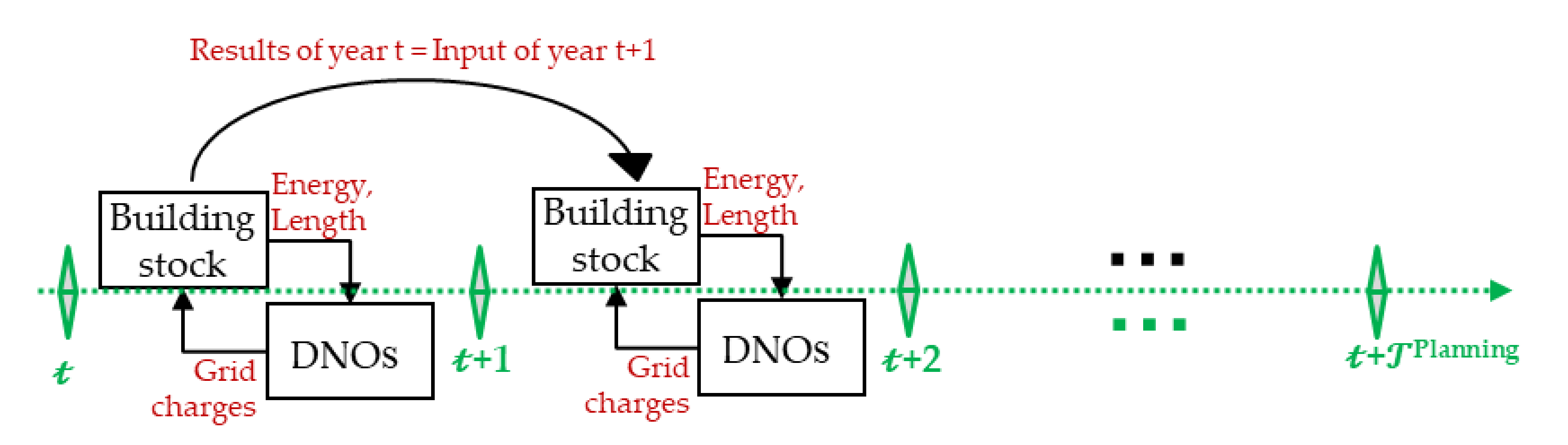
2.4. Procedure for the Analysis of Transformation Paths

Due to the reduction of complexity, we carry out the optimization for single years. To simulate a planning horizon of several years, the results from year 𝓉 are set as input values for year 𝓉+1 (Figure 3). By stringing together several simulations, we analyze the transformation path for a given planning horizon. A single building 𝒿 takes an investment in the year 𝓉 = 𝓉 I n v e s t when its heating system has reached its technical lifetime.

2.5. Conception of the Sensitivity Analysis

In the sensitivity analysis, we analyze the influence of interdependencies between building and DNO decisions on natural gas and electricity consumption in a transformation path from 2020 to 2050 for different types of building collectives and a regulatory scenario corresponding to the situation in Germany [22]. In each case, we assess the effect of a change in the grid topology, which is expressed by the exponent k (Equation (7)) on the development path. According to the ceteris paribus condition, within a scenario (represented by different types of building collectives), the effect of the change of an independent input variable (the exponent k) on the target variable (the standardized natural gas or electricity demand in 2050) is evaluated. Within a scenario, all parameters except for the input variable are constant over the entire analysis [56]. For a detailed description of the assumptions and simplifications in the validation (Section 3.3) and sensitivity analysis part (Section 3.4), see Appendix C, Table A4. In each scenario, we analyze a type of building collective consisting of 31 buildings of the same building type (classes: terraced house (TH), single family house (SFH), apartment building (MFH)) and age class (classes: B: 1860–1918, G: 1979–1983, K: 2010–2015) and connection ratios to the natural gas grid (classes: 100%, 75%, 50%), according to the German residential building typology [57]. Age class B represents buildings constructed before the foundation of the Federal Republic of Germany in 1948. Age class G represents buildings constructed according to Thermal Insulation Ordinances 1 and 2 (1979–1994), and age class K represents buildings constructed according to the revised Energy Saving Ordinance (2010-). The initial heating system types (AWHP: air–water heat pump, GCB: gas condensing boiler, OCB: oil condensing boiler, PB: pellet burner, EDH: electrical direct heating) are assigned to the buildings depending on their age class. Thereby, we distinguish three heating system configurations corresponding to different connection rates of the buildings to the gas grid (classes: 100%, 75%, 50%). The technical building equipment options (heating circuit characteristics, chimney, gas connection, etc.) are set corresponding to the type of heating system and the age class of the buildings; see Table A4. The combination of the three building types, age classes, and connection rates to the gas grid results in 27 types of building collectives, each of which is considered as a scenario in the sensitivity analysis (Table 2).
The number of years in the planning horizon corresponds to the number of buildings in the types of building collective (n = 31). Building renovations are equally distributed over the planning horizon, so one building is renovated every year. (Buildings with different initially installed heating systems are equally distributed over the planning horizon (see Appendix C, Table A4)).

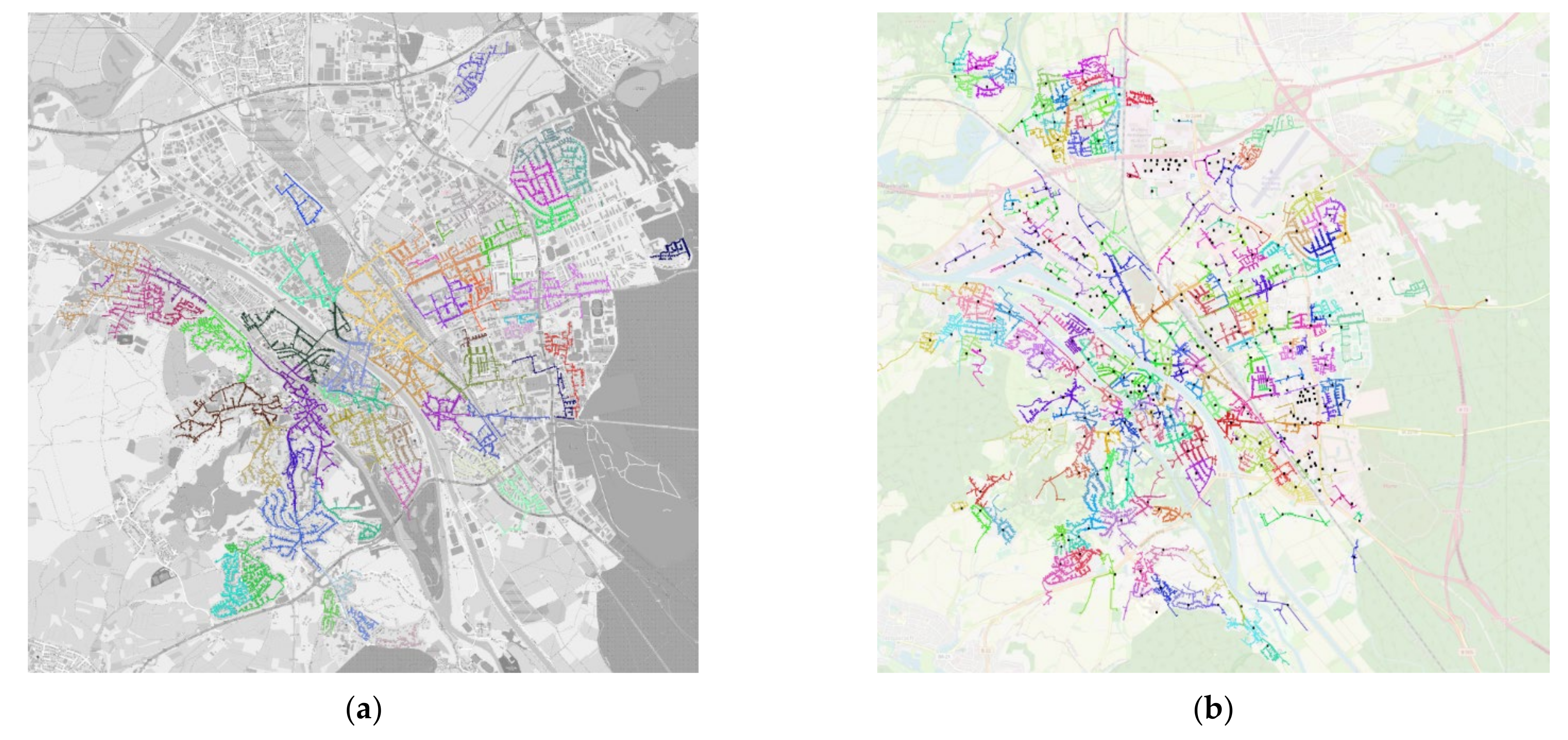
2.6. Grid and Building Data and Software Tools

To verify our assumptions and to estimate the ranges for the parameters of the sensitivity analysis, we analyze 58 real low-pressure natural gas grids and 323 low-voltage electricity grids as well as open source building data [58,59] of the southern German city of Bamberg, respectively the responsible gas and electricity DNO (Figure 4). The medium-voltage grid has a length of 277.8 km, and the low-voltage grid has a length of 932.7 km. The high-pressure network has a length of 0.7 km, the medium-pressure network has a length of 152.9 km, and the low-pressure network has a length of 217.7 km. The annual energy demand is 1282 GWh in the electricity and 858.5 GWh in the gas grid (2019). All buildings in the city area are connected to the electricity grid, but there are areas without a gas network. In those parts of the area where a gas network exists, about 80–90% of the buildings use gas for space or process heat generation. There is a special characteristic in the city area: The old town area is protected as a world cultural heritage site [59], so installations on the building envelope (e.g., photovoltaic (PV) system or heat pumps) are not permitted or are subject to approval. The electricity DNO has a revenue cap of approximately 20 M€ and the gas DNO has a revenue cap of approximately 10 M€. For the percentage distribution of the cost components, see [22]. The business figures and network data are provided by the DNO: Line and asset data are from the geo-information system; energy metering information is from the energy data management system; and the cost components of the revenue cap are from the cost allocation sheet. All data were recorded in 2018. The software-based models were created on a Python basis, using NetWorkX [60] for graph analysis and Pyomo [61,62] together with the commercial solver CPLEX [63] for the optimization. For load flow calculations, we use pandapower [64]. For pressure loss calculation, we use the commercial software STANET [65] and pandapipes [66].

3. Results and Discussion

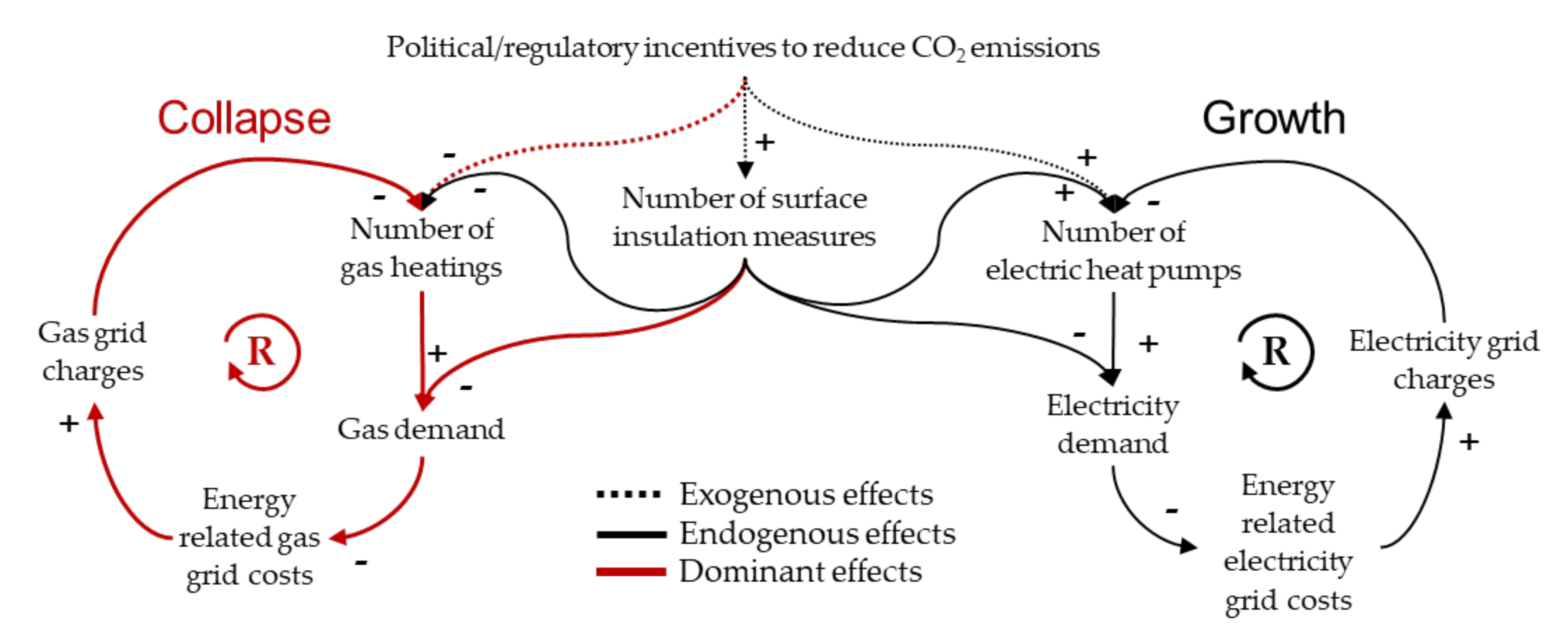
3.1. Identification of Influencing Parameters

In this section, we provide a literature-based answer to the following question: Which building-, heating-, and grid-specific factors influence significantly the transformation of the energy supply infrastructure and may foster non-gas-based systems? The results are used to select important parameters and scenarios for the structural grid (Section 3.3) and sensitivity analysis (Section 3.4). We define five classes of parameters: (i) state regulatory environment, (ii) grid charge models, (iii) market, technology, and environmental conditions, (iv) building, use, and ownership characteristics, and (v) DNO and grid characteristics, concerning the different actors’ policy, DNO, building, market, technology, and environment. For each of these factors, we have identified subtypes. Table 3 covers the description or interpretation of these subtypes and the literature sources used for the parameterization. In addition, we explain why we use each parameter as an objective variable (will be observed), for scenario generation, or as an input variable, which will be varied in the sensitivity analysis (Table 3).

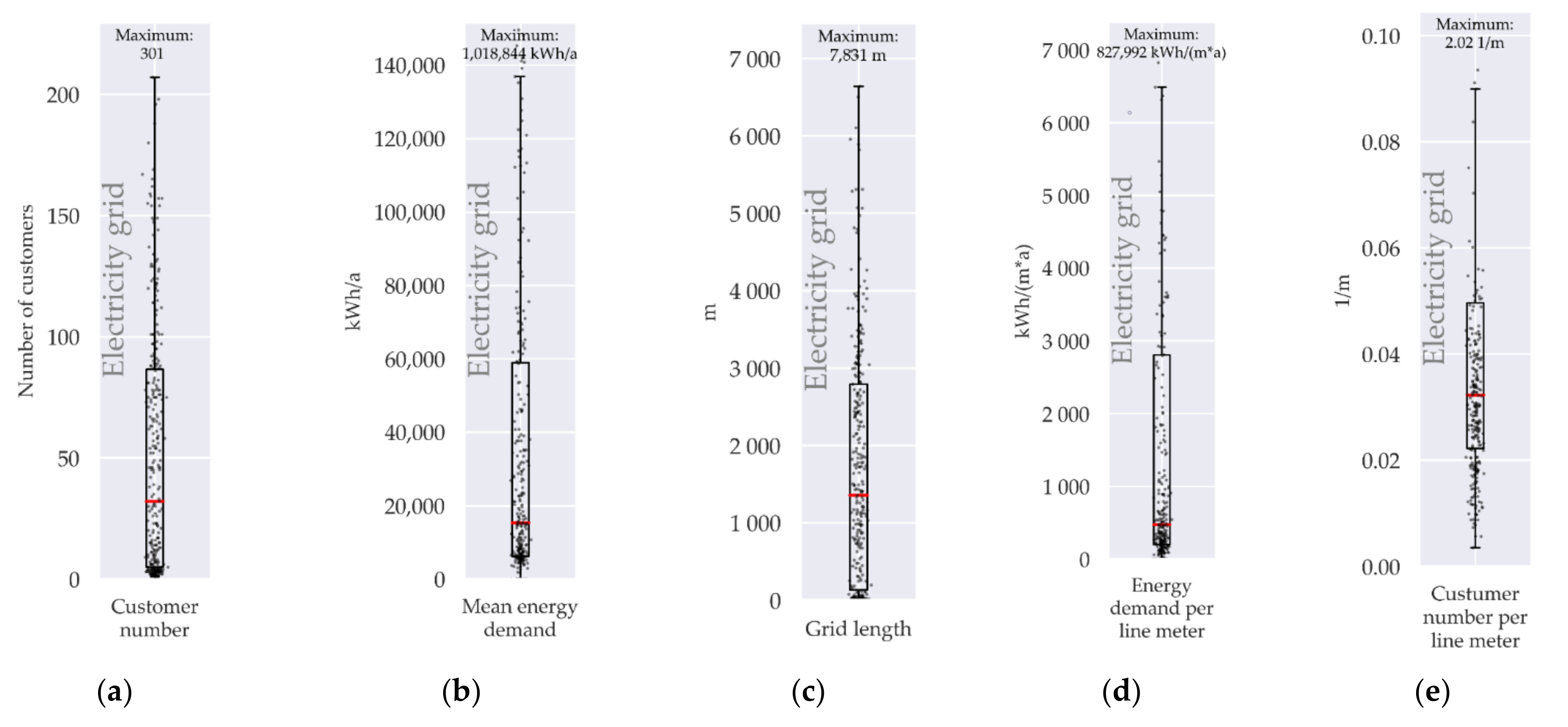
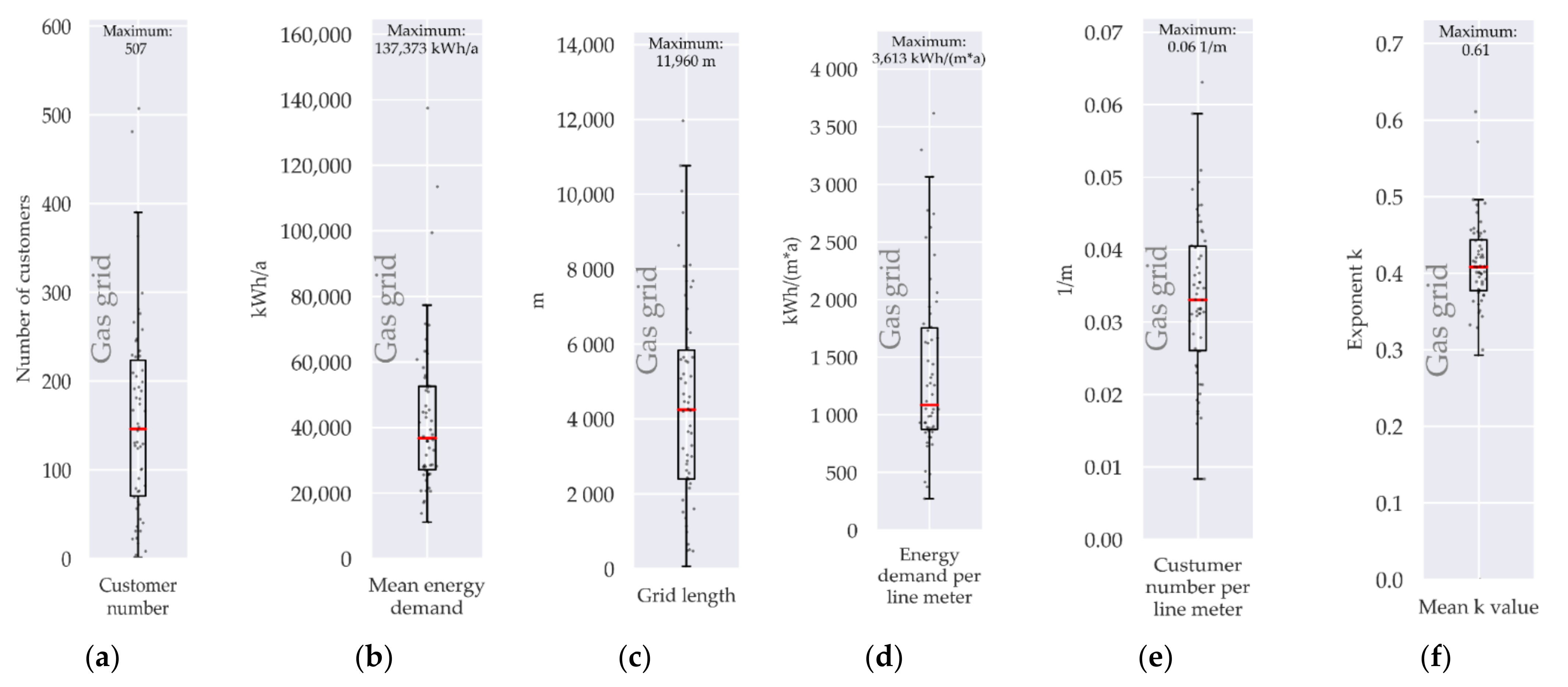
3.2. Analysis of Selected Structural Parameters for Real Urban Grid Areas

In this section, we answer the following question: How were building-, heating- and especially grid-specific influencing factors shaped in real urban grid areas of the German city of Bamberg in 2019? Therefore, 58 natural gas and 323 electricity distribution grids will be investigated. The results are used to define the scenarios and parameter settings for the sensitivity analysis (Section 3.4.). We analyze selected structural parameters that have a high influence on the grid economics [16]:
  • The number of customers supplied as well as the network length serve to classify the size of the investigated grid gas and electricity areas;
  • The energy demand and the number of customers per meter of line are used to classify the demand or customer density;
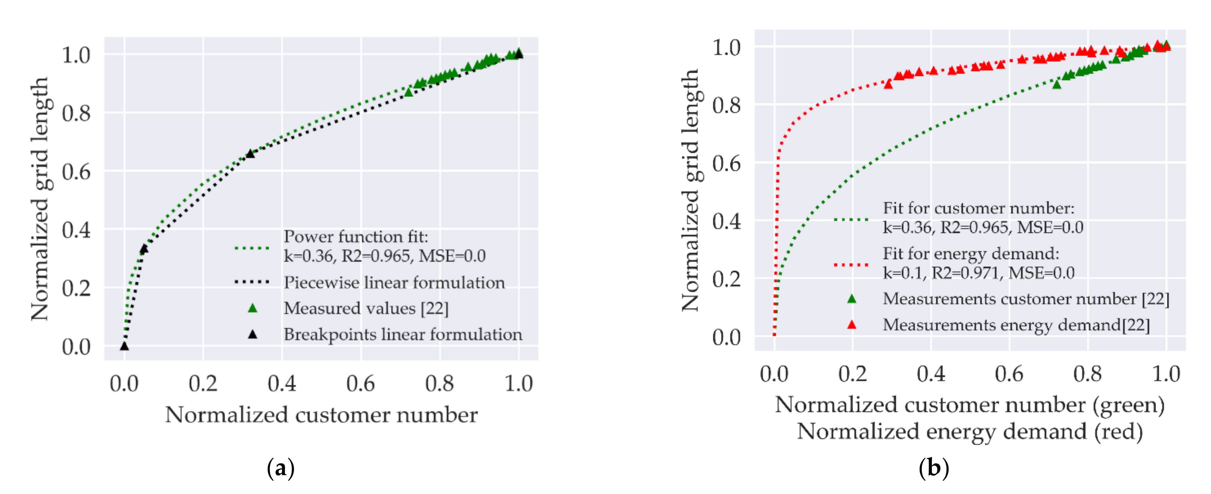
  • The average annual energy consumption of buildings provides information on the average customer size; the exponent k describes the grid topology and serves as a measurand for the relationship between the number of customers and the grid length needed for supply. This is the median of 10,000 simulations in which the customers are randomly removed from the grid one after the other. During this procedure, we have classified the grid length needed for supply and finally performed a power function fit to estimate k for every grid (n = 58) and simulation (n = 10,000) [16].
Figure 5 shows the results for the gas grids. The median in grid length is 4225 m, and the median of the number of customers is 146. The average energy consumption differs between 27,000 kWh (0.25-quantile) and 53,000 kWh (0.75-quantile), which is induced by a fluctuating connection density of the buildings to the gas grid as well as their size and energy efficiency. The number of customers per line meter (connection density) is between 0.026 L/m (0.25 quantile) and 0.04 L/m (0.75 quantile). This means that the distance between buildings connected to the gas grid is between 25 m (0.75-quantile) and 38 m (0.25-quantile). This range corresponds to comparable studies ([17]: Adoption for high-density areas 0.048 and low-density areas 0.021.). In the sensitivity analysis, we set the building density on a fixed level (0.04 L/m) and vary the heating system configuration of the building stock in three scenarios, whereby 50%, 75%, or 100% of the buildings are connected to the gas grid. This leads to connection densities of the buildings to the gas grid of 0.02, 0.03, and 0.04 L/m, corresponding to the situation in the real grid area of Bamberg.
The energy demand per line meter in the grid area is between 872 (0.25-quantile) and 1753 kWh/(m*a) (0.75-quantile). In a comparable study [17], the variation is higher: 5760 kWh/(m*a) for high-density areas with large connections and 840 kWh/(m*a) for low-density areas with small connections. Our scenarios in the sensitivity analysis cover a similar wide range of values: In the case of an apartment building stock of building age class B (MFH-B), a 100% connection rate results in an energy demand per line meter of approximately 4800 kWh/m and of approximately 400 kWh/m in case of a single-family house stock in the age class of K (SFH-K) with a connection ratio to the gas grid of 50%.
The exponent k, which describes the relationship between the number of customers in the grid and the network length, varies between 0.377 (0.25-quantile) and 0.443 (0.75-quantile). The dispersion of the value depends on the network topology and the order, respectively the distribution of the customer exits. We select the customer exits randomly. If this distribution is weighted, larger or smaller values of k are possible [16]. For that reason, we vary the exponent k as an input parameter in the sensitivity analysis from 0.2 to 1.0 in 0.2 steps.
The electricity and gas grid areas are not congruent; also, their characteristics differ: The number of electricity grids (n = 323) is significantly higher than that of the gas grids (n = 58); the grid length of the electricity grids (1351 m) is smaller than that of the gas grids (4225 m, 0.50 quantiles); the number of customers in the electricity grids (n = 32) is smaller than in the gas grids (n = 146, 0.50 quantiles); and the average energy demand of a customer in the electricity grids (15,301 kWh/a) is also lower than in the gas sector (36,725 kWh/a, 0.50 quantiles). The customer number per line meter in the electricity sector is 0.032 L/m, which is comparable to a similar level of 0.033 L/m in the gas sector (0.50 quantiles), although the dispersion in the electricity is higher than in the gas sector (IQD electricity 0.027 L/m, IQD gas 0.014L/m). As a result, the energy demand per line meter in the electricity sector (474 kWh/(m*a)) is lower than in the gas sector (1085 kWh/(m*a), 0.50-quantile). The dispersion is higher in the electricity than in the gas sector; compare Figure 5 and Figure 6.

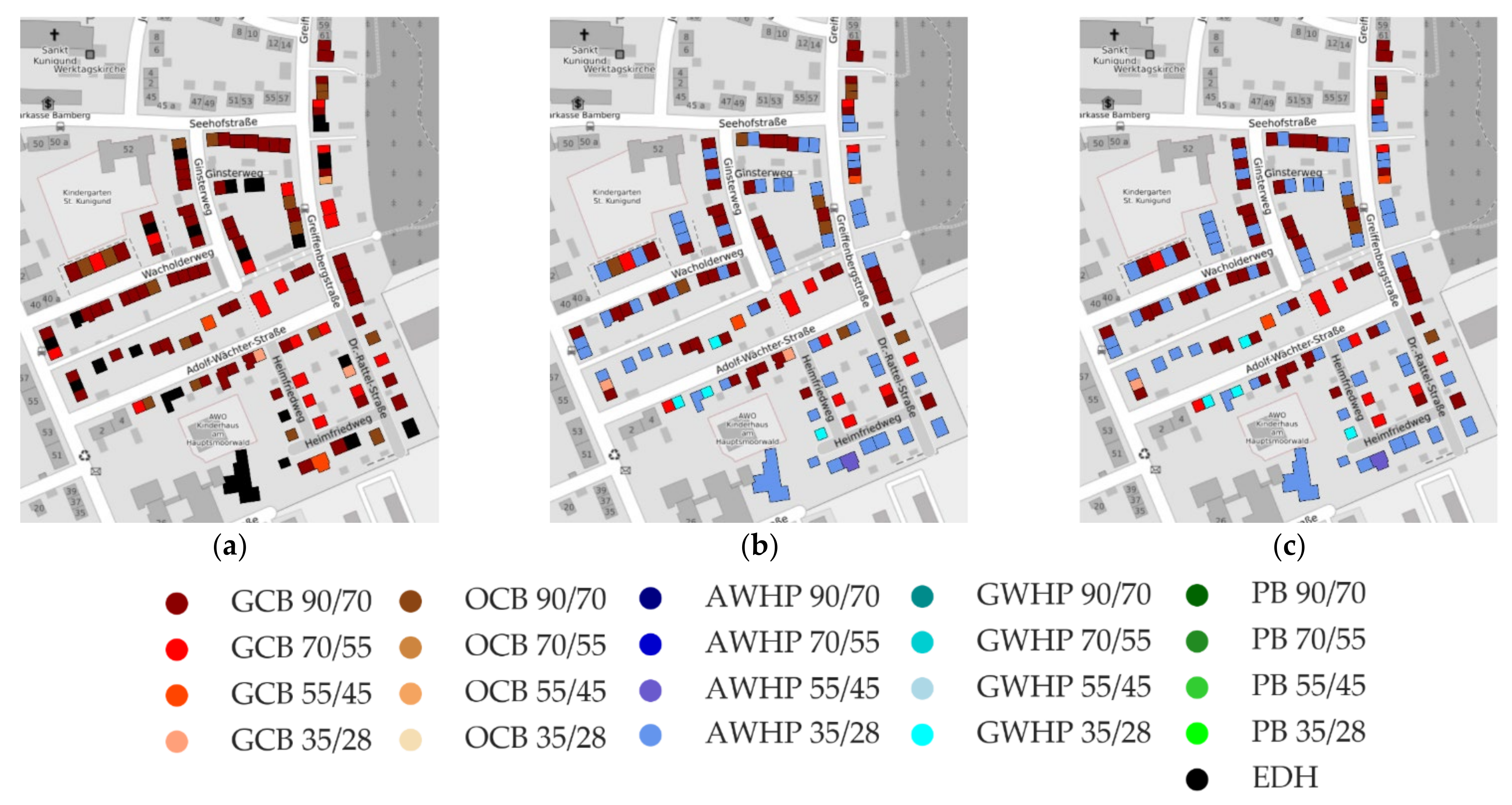
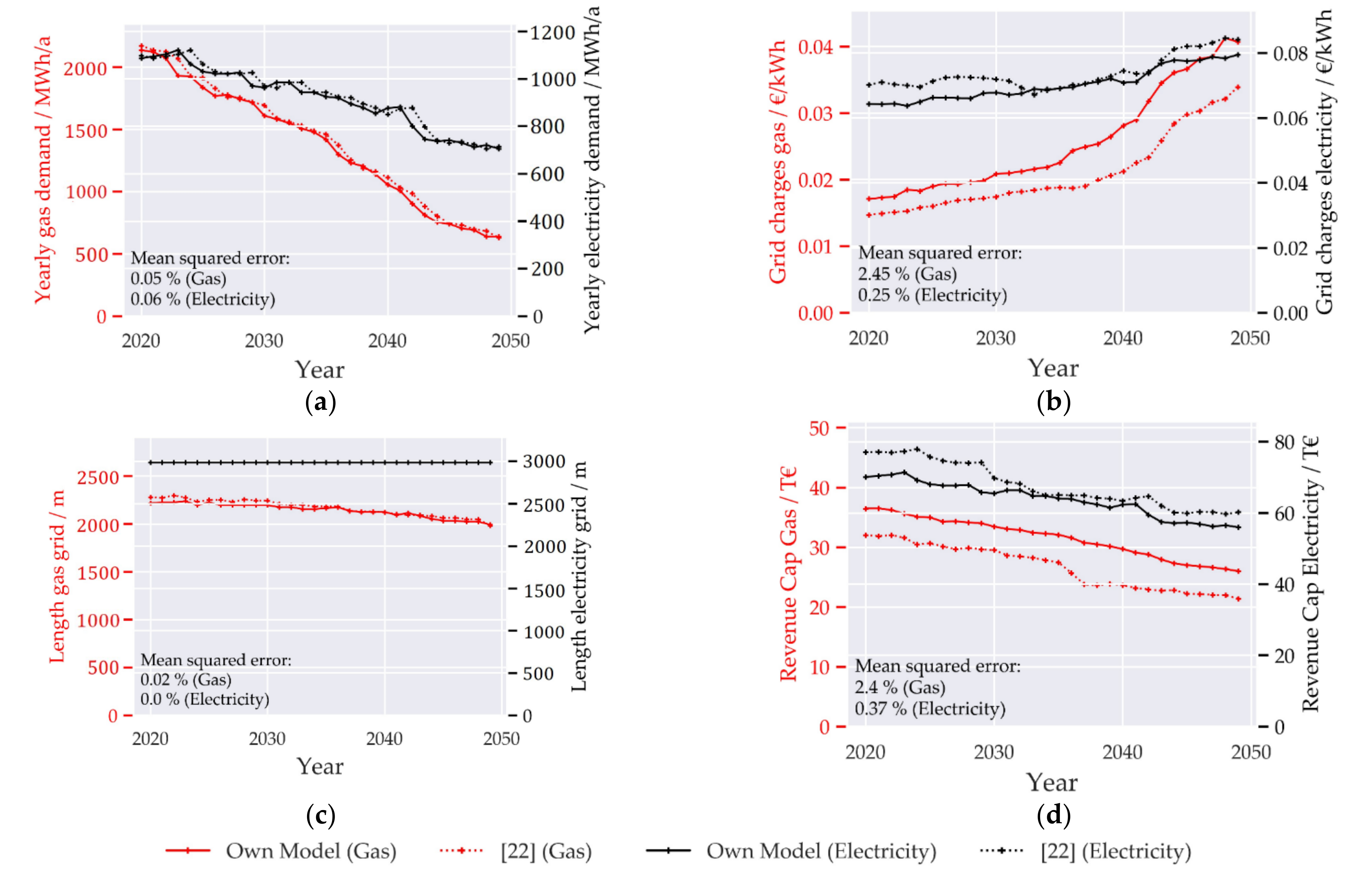
3.3. Model Validation and Transformation Path Analysis of a Real Grid Area

In this section, we address two questions: (i) How are the endogenous variables (gas and electricity demand and the corresponding grid charges) shaped within the transformation path? (ii) Does our simplified grid and DNO model provide valid results? To answer these questions, we perform a simulation with our MILP model from 2020 to 2050 for a real electricity and gas grid area in the German city of Bamberg. This grid area was already analyzed in [22] based on a multi-agent simulation (MAS) with a similar building retrofit model and a detailed grid and DNO model, considering the individual grid assets. Thus, we are able to validate our results regarding the buildings’ investment decisions (heating system type, insulation status), the power function fit (customer number and grid length), as well as the gas and electricity DNO’s characteristics (grid charges, energy demand, grid length, revenue cap). The insulation status of the buildings, building types, and the corresponding heating systems are determined on the basis of [22] open street maps [59] and IWU-type buildings (IWU: institute of housing and environment), compliant with the data protection act [74]. For additional assumptions, simplifications, and adjustments corresponding to [22], see Appendix C.
The initial building stock is characterized by terraced houses of age classes F and G (n = 95) and single-family houses of age class E (n = 11), which are primarily equipped with gas (n = 86) and oil burners (n = 17) or electric direct heatings (n = 17) (Figure 7a). There are only minor differences between the selected building retrofits of both simulations ([22] in Figure 7b and our model in 7c): 5.4% (n = 7) of the buildings choose a divergent heating system configuration consisting of the heat generation unit and the heating circuit; 0.8% (n = 1) of the buildings choose different insulation thicknesses (difference greater than 5 cm); 0.8% (n = 1) of the buildings choose a solar thermal system of varying size. These differences are due to two reasons: Firstly, we restrict the solution space by limiting the choice of insulation thicknesses and solar thermal systems in order to reduce the computing time, compared to [22]. Secondly, our model maps the interdependency between the two actors is within a time step: We integrate both problems, the building owner’s retrofit and the DNO’s investment decisions, in a joint model. In the MAS from [22], both problems are modeled independently from each other in their own agents, which interact before and after optimization. As a result, the original optimization problems of both actors (building and DNO) are decoupled within a time step.
Some general trends can be deduced from the results of both simulations (for this area under the assumed regulatory constraints):
  • Electric direct heatings are substituted without exception due to the energy price and the regulatory constraints, mainly by electric heat pumps (25 out of 26 systems in [22]).
  • Energy prices and the regulatory constraints lead to an increased substitution of oil (eight of 17 systems in [22]) and gas burners (27 of 86 systems in [22]).
  • Measures in the range of 10–20 cm are chosen for building insulation. In those cases, oil and gas burners (84% of the buildings with insulation measures in [22]) become more attractive than heat pumps (16%).
  • Solar thermal systems are only installed in a small number (n = 6) and mainly used in apartment buildings (four out of six buildings in [22]).
We model the relationship between grid length and number of customers using a power function and estimate the exponent k based on the results from [22] (see Figure 8b, green curve). After fitting, we linearize the function piecewise. The breakpoints are selected so that the sum of the error squares is minimized (Figure 8a).
This represents a significant simplification of the grid and DNO model. Therefore, we validate our model in the following way. Based on the results of [22], an additional observation can be made: Energy-saving measures increase the disproportionality between the length of the grid and the energy supplied (Figure 8a). Due to the properties of the potency function, we systematically underestimate the length. This effect could further accelerate the grid charge increase in scenarios where grid customers leave the grid.
The validity of our simplified grid and DNO model can be assessed by comparing the gas and electricity demand (Figure 9a), grid charges (Figure 9b), grid lengths (Figure 9c), and revenue cap (Figure 9d) development of both simulations.
In the case of electricity and gas demand, as well as the gas grid length, the error is small. The absolute value of the revenue cap and the grid charges in the gas sector are overestimated in our model. This additive error is due to the simplifications within our model and comes from an overestimation of the CAPEX, rather than the cumulative modeling of all assets with the mean rest book value mrbvf 𝒸 , 𝓉 . This systematic error can be compensated by adjusting the specific cost parameter C 𝒸 I of the lines (historical acquisition costs) of the DNO. As a result, the revenue caps and grid charges for gas and electricity of the two simulations would coincide at the beginning of the simulation.
In both simulations, some general trends for the interdependencies between the actors can be observed: The gas demand decreases, which is induced by energy-saving measures and the substitution of gas-based systems (Figure 9a). Consequently, the grid charges increase by 134% from 2020 to 2050, resulting in an increase in the gas procurement price of 36% (own model, Figure 9b). Depending on the type of building and the initial building equipment, this can increase the total costs of the gas-based retrofit solution to such an extent that heat pump solutions appear economically more attractive. As a result, the rate of change in gas demand over time increases from 2035 up to 2050 compared to the period 2020–2035.
The observed increase in grid charges is mainly induced by the disproportionately low decrease in grid length (Figure 9c) in relation to energy: By 2050, the gas demand will decrease by approximately 70% and the length of the grid will decrease by approximately 10%. As a result, a disproportionately long grid has to be operated. The resulting costs for network operation are allocated to the grid charges, which is why the revenue cap of the gas DNO decreases almost linearly (Figure 9d). The decrease in electricity demand in this grid area is induced by the change of the initially high number of electrical storage heaters and energy-saving measures in the buildings, also resulting in an increase in grid charges.

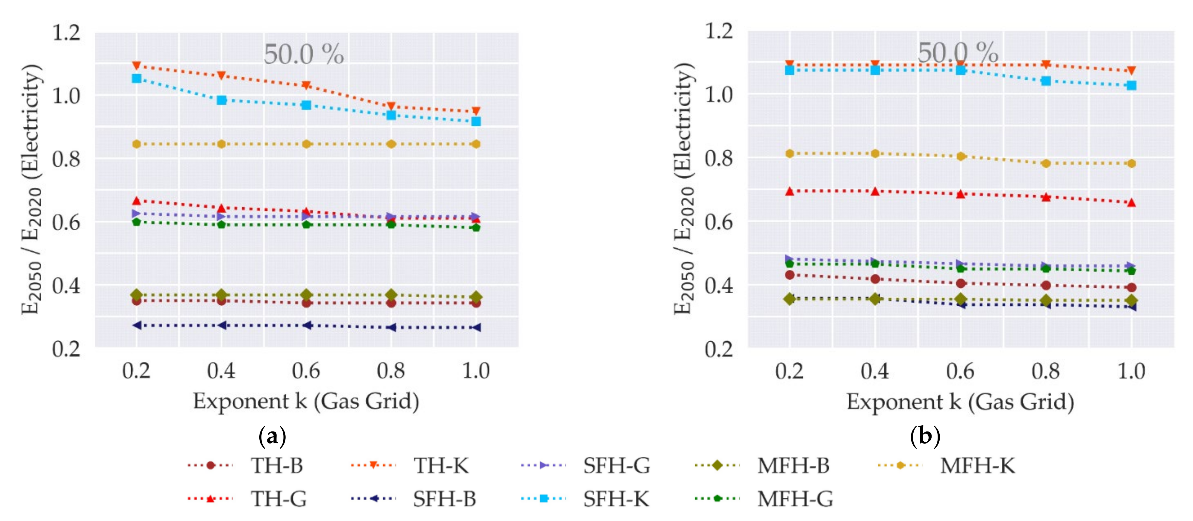
3.4. Sensitivity Analysis for Types of Building Areas

In the sensitivity analysis, we address the following questions: (i) How are the endogenous variables (gas demand, gas grid charges) influenced by different configurations of the exogenous variables (building type and age, heating system configuration, grid topology)? (ii) Which configuration of exogenous variables results in an equilibrium between the construction and replacement of gas-based heating systems, fosters gas-based systems, or causes the collapse of the gas grid infrastructure?
For that reason, we simulate different scenarios for a building collective (n = 31), varying the building types (n = 3), the building age classes (n = 3), and the initial heating system configuration (n = 3) (period: 2020–2050). For each scenario, we perform the simulation for five grid topologies (represented by the exponent k). In addition, we investigate how the initial grid age and the interest rate for energy procurement in the buildings influence the results. We measure the gas and electricity demand in 2050 in relation to 2020 and discuss the heating system stock in 2050.
Figure 10 shows the development of the relative gas demand for all types of building collectives (lines) and grid topologies (data points). For the electricity demand, see Figure A1 in Appendix D. One data point represents the gas demand (2050 compared to 2020) of one simulation (the same building, heating and grid configuration): The gas demand decreases for all types of building collectives (building types: TH, SFH, MFH, age classes: B, G, K), particularly in areas with terraced and single-family housing and a low ratio of buildings connected to the gas grid (connection rates: 50%, 75%, 100%). With regard to the connection rate, a dependence of the gas demand to the network topology (value k) can be observed, which decreases with an increasing value of k. This means that the risk of a complete gas grid defection increases with a decreasing initial connection rate of buildings to the gas grid, building size (SFH, TH), and a decreasing exponent k (compare Figure 10a–c). Hence, the exponent k, which describes the network topology, can also be seen as a predictor for the risk of gas grid defection: For smaller values of k, the disproportionality between grid length and energy supplied rises. With that, the risk of a grid charge increases when customers leave the grid. This effect fosters the attractiveness of a substitution of gas-bound systems but weakens the higher the connection rate of gas customers or energy consumption per line meter.
Two opposing mechanisms can be observed in buildings with initially installed gas burners, especially in areas with a lower ratio (50% or 75%) of small buildings (SFH, TH) connected to the gas grid: On the one hand, the initial gas grid charges and thus energy-related expenditures for gas burners are on a high level, which make gas burners unattractive for new construction. On the other hand, buildings that initially use gas burners tend to renew them, as long as energy-related expenditure remains below a certain threshold, as the conversion is associated with additional costs.
A change of the energy carrier for heating is associated with a retrofit of the technical building equipment, which increases the investment expenditures. This concerns buildings that switch to gas as well as from gas, so there is an interrelation between both mechanisms.
In areas with a low connection rate (50%, 75%), the non-gas-supplied buildings of the age class K have initially installed heat pumps, while those of the age classes B and G have initially installed oil burners and electric direct heating systems. Each system is linked to the corresponding technical building equipment option. In the case of direct electric heating, the installation of a gas condensing boiler is associated with a retrofit of a gas grid connection, a chimney, and a heating distribution network, as well as radiators. In our model, these expenses are partly independent and partly dependent on the size of the building (reference floor area). Consequently, the weight of the investment expenditure for the technical building equipment in the investment decision is higher in SFH and TH compared to MFH buildings. In MFH buildings, the investment and operating expenditure for the heat generator are higher weighted (compare Figure 11a–c).
On the one hand, this makes the substitution of an existing gas burner unattractive as long as the energy-related expenditures do not rise above a certain threshold. On the other hand, even for low energy-related expenditures, switching to gas burners is prevented by high investment expenditures for retrofitting the technical building equipment.
An additional aspect to be observed concerns the renovation of the building envelope: Corresponding to the expected technical lifetime of the building envelope of about 47 years, 66% of the buildings renovate the building envelope within the planning horizon. The discussed cost situation concerning the technical building equipment motivates building owners to take insulation measures when renewing their gas heating systems, especially in areas with small buildings (SFH, TH). Even in other types of building collectives (MFH), surface retrofits are often combined with the installation of a gas burner, especially in buildings with initially installed gas burners. We see this by comparing Figure 10a with Figure 11a (type: MFH-K, 50% connection rate, k = 0.6): The number of gas systems remains unchanged, but the gas demand drops by 42% from 2020 to 2050, which is induced by insulation measures and the use of solar thermal systems. Thus, for certain MFH-type collectives, the relative gas demand decreases (compare Figure 10a–c, types: MFH-B and MFH-G) with an increasing number of gas-bound systems (compare Figure 11a–c).
In this context, it is important to note that the grid charges are calculated individually for each building collective. Therefore, they are lower in areas with multi-family housing than in those with terraced or single-family housing: We take into account the grid charges of the transportation grid by means of a fixed cost parameter C 𝒸 UpGC , which is defined globally for all areas. The grid charges of the distribution grid are calculated individually based on the characteristics of the grid and the energy demand. Since the grid length and age of the distribution grid are defined globally, the grid charges vary between the building collectives depending on the energy demand of the individual areas. This corresponds to the methodology used in practice [17]. As the building stock in real grid areas is much more heterogeneous, the dispersion of grid charges between areas is less pronounced than that between our type collectives.
In the following, we extend the sensitivity analysis by varying two parameters that have a major influence on the development, namely the initial length-weighted network age on the gas and electricity DNO side [17] and the interest rate for energy procurement expenditure on the building owner side:
  • The initial length-weighted grid age has a major impact on the level of the grid charges. It largely determines the DNO’s CAPEX, which is dependent on the grid length and age. We vary the base setup (electricity and gas grid age of 0.50 · T TL ) to a grid age of 0.75 · T TL .
  • The building owners’ investment decisions are significantly influenced by the level of the interest rate for energy procurement expenditure. We model them as an annually constant expenditure series for the technical lifetime of the heating system (33.5 years) and an interest rate of 4% (PF = 18.3). We vary the rate of the base setup to a rate of 0.5% (PF = 31).
Figure 12 shows the results of the analysis of a change in the grid age (Figure 12a) and interest rate (Figure 12b) for energy procurement expenditure. The connection rate of buildings to the gas grid in both simulations is 50%. Figure A2 in Appendix D shows the sensitivities of electricity demand to changes in interest rates and grid age.
An initial grid age of 0.75 · T TL (Figure 12a) results in a higher gas consumption and a lower dispersion compared to the basic setup (Figure 10a), especially for small values of k and the type areas TH-K and SFH-K. This effect occurs as long as the optimizer tries to keep the initial grid age constant but is reversed as soon as it tries to reduce the grid age to the level of 0.50 · T TL by increasing the investments, as it is assumed in other studies [17].
A reduction in the interest rate for expenditure on energy procurement (Figure 12b) has the opposite effect: The dispersion increases, and scenarios in which the gas grid is totally defected becomes more likely. With a decreasing interest rate, the weight of the energy-related expenditure in investment decisions increases. As a result, an increase in grid charges has a stronger effect on the investment decision. In this sense, the interest rate represents a weighting factor for energy-related expenditure in the building investment decision. In reality, a reduction of the interest rate corresponds to investors who put more emphasis on operating than on the investment expenditures [71]. In this case, the risk for gas grid defection increases.

4. Conclusions

Our work provides two innovations in modeling: We present a single-level mixed integer linear program with which retrofit decisions of buildings and investment decisions of electricity or gas DNOs can be evaluated in an integrated way, i.e., with the mutual dependencies between the different actors. We achieve this goal by (i) transforming the central DNO optimization problem considering the yearly cash flow to an equality constraint, (ii) mapping the relationship between grid length and supplied energy in the grid by a validated power function fit, and (iii) integrating the whole sub-model into the original building retrofit optimization model.
A validation using a detailed grid and DNO model [22] has shown that our simplified model provides high-quality results. As the grid is only determined by its age, the exponent k, the grid length, customer number, and the DNO’s cost parameters, this simplified model can be used in macroscopic studies where many subnetworks have to be modeled, which are often lacking detailed information. For that reason, our model can be used independently of the building model. It helps to improve the quality of studies that currently neglect the grid topology [25].
On the one hand, the results of the transformation path analysis for the building sector confirm general trends from the literature (considering the situation in Germany) [14,22]. (i) Electric direct heating systems are substituted without exception. (ii) Energy prices and the regulatory conditions lead to an increased substitution of oil- and gas-based systems by electrical heat pumps. (iii) In case of building insulation, oil and gas burners become economically more attractive. On the other hand, the results of the transformation path analysis offer some new insights into the interrelated system between gas and electricity grid investments and the building owner’s retrofit decisions: As the gas demand decreases, which is induced by energy-saving measures and heating system changes in buildings, the gas grid charges rise, which makes the substitution of gas-fired heating more attractive and thus accelerates the decrease in gas demand.
The results of the sensitivity analysis for 27 different types of building collectives and five different network topologies show that the transformation path strongly depends on the building, heating system, and network configuration whereby two trends can be observed depending on the individual configuration.
On the one hand, gas-fired systems are currently attractive for building owners in areas with apartment housing (MFH) and a high density of buildings connected to the gas grid. This is because the initial grid charges are low and the investment expenditure for the technical building equipment for the installation of a gas condensing boiler (heating circuit, chimney and gas connection) is low in relation to absolute investment expenditure in case of MFHs. From a DNO’s point of view, the economic viability of the gas network in these areas is secured for the future, even if the demand for gas is declining.
If, on the other hand, heating energy demand decreases in areas with single-family or terraced housing (SFH, TH) with a lower rate of buildings connected to the gas grid, the grid charges that are initially at a high level rise sharply, further reducing the attractiveness of gas-based systems. For these areas in particular, the long-term question at a political level is whether it makes economic sense to operate a gas network. For areas where this is not the case, the respective federal policy should provide building owners as well as DNOs incentives to substitute gas-bound heating systems and deconstruct the gas grid infrastructure. In areas in which the operation of the gas network is also economically viable in the future due to the energy demand and network structure, the increasing grid charges to be borne by the individual grid user should be socialized. This reduces the risk of a complete gas grid defection and helps to maintain the gas grid in particular, as the natural gas infrastructure can serve as a flexibility option in a future renewable energy system [75]. The conversion of the grid charge system is a suitable option to maintain or shutdown grid infrastructure at a local level [34].
The insights gained in the sensitivity analysis on specific building structures can be used in practice to reduce economic risks (sunk costs) in relation to grid renewal measures: In a first step, it is possible to cluster the building stock within the grid area according to the presented characteristics. In a second step, critical areas with a high risk of gas grid defection can be identified and investment roadmaps adapted. For that reason, our approach has to be extended for industrial and commercial areas with particularly high load density. Therefore, heating grids have to be integrated in the model, as they are economically attractive in high-density building stock [76,77]. Furthermore, we have not considered the usage of renewable gases and hydrogen in the future energy system (our assumption: CO2 footprint in grid-bound gas supply remains unchanged on the initial level). A reduction of the CO2 footprint would raise the attractiveness of gas-bound systems, especially in areas with a high density of gas grid connections and small buildings (due to the ratio of investment expenditures for the technical building equipment and the heating).

Author Contributions

Conceptualization, D.T. and T.M.K.; data curation, J.B.; Formal analysis, M.B.; funding acquisition, T.M.K. and M.B.; investigation, D.T. and J.B.; methodology, D.T.; software, J.B.; supervision, M.B.; visualization, D.T.; writing—original draft, D.T.; writing—review and editing, T.M.K. and M.B. All authors have read and agreed to the published version of the manuscript.

Funding

This research received no external funding.

Acknowledgments

We would like to thank the Stadtwerke Bamberg energy and water supply company, Bamberg, Germany, for providing us the data of loads, grids, and costs components that form the basis for this work.

Conflicts of Interest

D.T. is an employee of the Stadtwerke Bamberg GmbH. The authors declare no conflict of interest.

Appendix A. Nomenclature

Table A1. List of acronyms.
AcronymNameAcronymName
AWHPAir water heat pumpMPPDCMathematical program with primal and dual constraints
BESBuilding energy systemMASMulti-agent simulation
BEBuilding envelopeMFHMore family house
BBuilding age classMSEMean squared error
BOBuilding ownerOCBOil condensing boiler
CAPEXCAPEXOPEXOPEX
CO2Carbon dioxideOSMOpen street maps
COPCoefficient of performance (heat pumps)PBPellet burner
DHWDomestic hot waterPFPresent value factor
DNODistribution network operatorR2Coefficient of determination
EEnergyRFAReference floor area
EDHElectrical direct heatingRBVRest book value
ERRExpected rate of returnRCRevenues cap
EUEuropean UnionSTESolar thermal plant
GCGrid chargesSFHSingle family house
GCBGas condensing boilerSGCStable grid charges
GWHPGround water heat pumpSGVStable grid value
IQDInterquartile distanceSRCStable revenue cap
IWUInstitute Housing and EnvironmentSTESolar thermal energy plant
MILPMixed integer linear programTHTerraced house
Table A2. Nomenclature of formula symbols of the building retrofit model, see also [22].
ParameterDescription [Unit]ValueSource
Components of the expenditures
c 𝒿 B Total expenditures for heating within the technical lifetime of the heating system [€]
c 𝒿 BE Investment expenditures for the building insulation retrofit [€]
c 𝒿 BES Investment expenditures for the change of the heating system and technical building equipment [€]
c 𝒿 EN Expenditures for energy procurement over the technical lifetime of the heating system [€]
c 𝒿 M Expenditures for maintenance over the technical lifetime of the heating system [€]
Parameters
A 𝒿 E Building surface area [m2]Corresponding values are shown in [22] (Supplementary Materials)
A 𝒿 , 𝓅 EP Area of a building surface component [m2]
T 𝒿 N Yearly usage hours of the heating system [h]
S 𝒹 , 𝒿 BE Design-relevant building heat load (for heating system) (thermal ventilation and transmission losses) [kW]
S 𝒿 S Heat load for: Radiation losses, internal wins, heat distribution losses, auxiliary energy [kW]
S 𝓈 , 𝒿 STE Heat load thermal solar plant [kW]
S 𝒿 DHW Heat load for domestic hot water generation [kW]
M 𝓀 BES Specific yearly expenditures for maintenance of the heating in percent of investment expenditure [-]
M 𝓈 STE Specific yearly expenditures for maintenance for the solar thermal plant in percent of investment expenditure [-]
E 𝓀 BES Plant expenditure figure of the heating systems
B 𝒸 , 𝓀 EC Energy carrier of the heating system (Binary decision parameter)
C 𝒿 BEvar Specific variable investment expenditures for a building surface retrofit [€/(m2·cm)]
C 𝒿 BEfix Specific fix investment expenditures for a building surface retrofit [€/m2]
D 𝒹 D Insulation thickness [cm]0–30
C 𝓀 BESvar Specific variable expenditures for the heating system [€/kW]Corresponding values are shown in [22] (Supplementary Materials)
C 𝓀 ,   𝒿 BESMfix Specific fix expenditures for the heating system (maintenance) [€]
C 𝓀 ,   𝒿 BESfix Specific fix expenditures for the heating system [€]
C 𝓈   STEvar Specific variable expenditures for the solar thermal plant [€/kW]
C 𝓈 STEfix Specific fix expenditures for the solar thermal plant [€]
C 𝒸 , 𝓉 EC Specific yearly energy related expenditures (tax + procurement + grid charges) [€/kWh]
C 𝒸 , 𝓉 Proc Specific energy procurement costs Electricity [€/kWh]0.0761[78]
Natural gas [€/kWh]0.0313[78]
Oil [€/l]0.506[79]
Pellet [€/kg]0.231[80]
C 𝒸 , 𝓉 Tax Energy related taxes and duties (excluding the CO2 tax, which is calculated in the model)Electricity [€/kWh]0.1602[78]
Natural gas [€/kWh]0.0164[78]
Oil [€/l]0.169[81,82]
Pellet [€/kg]0.016[81,82]
EM 𝒸 , 𝓉 EC Specific CO2-emissions per energy carrier [kg/kWh]Electricity (linear decrease to 0.103 in 2050)0.462[83,84]
Natural gas0.202
Oil0.294
Pellet0.023
HV 𝒸 Heating value Natural gas [kWh/m3]11.42[85]
Oil [kWh/liter]11.27
Pellet [kWh/kg]5.27[86]
F 𝒸 P Primary energy factorElectricity1.8[19]
Natural gas1.1
Oil1.1
Pellets0.2
Q 𝒿 H init Initial yearly end energy demand of a building
EM 𝒿 init Initial yearly CO2 emissions of a building
Q 𝒿 P EnEV Upper bound for the yearly primary energy demand considering the energy efficiency constraint
S 𝒿 T EnEV Upper bound for the heat load considering the energy efficiency constraint
PF M Present-value factor maintenance31
PF EN Present-value factor energy procurement31 or 18.3
Variables
b 𝒹 , 𝒿 B E Building surface retrofit 𝒹 in house 𝒿 (Binary decision variable)
b k ,   𝒿 B E S Heating system 𝓀 in house 𝒿 (Binary decision variable)
b 𝓈 , 𝒿 S T E Solar thermal plant 𝓈 in house 𝒿 (Binary decision variable)
e 𝒸 , 𝓉 Heating Energy for heating applications in year 𝓉 in gas or electricity grid [kWh/a]
E 𝒸 , 𝓉 AnyOther Energy for all applications except heating in year 𝓉 in gas or electricity grid [kWh/a]
c 𝒸 , 𝓉 G C Grid charges gas or electricity in year 𝓉 [€/kWh]
Indices and sets
𝒹 D An insulation thickness standard 𝒹 of all standards 𝒟
𝓅 P Surface part 𝓅 of all building surface parts 𝒫
𝓀 K . A heating system type 𝓀 of all heating system types 𝒦
𝒸   ϵ   C An energy carrier 𝒸 of all carriers 𝒞
𝓈 S A solar thermal plant 𝓈 of all available types and sizes 𝒮
𝒿   ϵ   𝒿 A building 𝒿 of all buildings 𝒥 connected to the grid
Table A3. Nomenclature of the distribution network operator model, see also [22].
ParameterDescription [Unit]ValueSource
GasElectricity
Cost components of the revenue cap
α 𝒸 , 𝓉 C A P E X Capital expenditures gas or electricity [€]
α 𝒸 , 𝓉 O P E X Operational expenditures gas or electricity [€]
α 𝒸 , 𝓉 E C Calculated return on equity gas or electricity [€]
α 𝒸 , 𝓉 B C Interest on borrowed capital gas or electricity [€]
α 𝒸 T a x Calculated trade tax gas or electricity [€]
α 𝒸 , 𝓉 D e p r Calculated interest on borrowed capital gas or electricity [€]
α 𝒸 , 𝓉 O C Operational costs gas or electricity [€]
α 𝒸 , 𝓉 L C Loss costs gas or electricity [€]
α 𝒸 , 𝓉 U p G C Upstream grid charges gas or electricity [€]
α 𝒸 , 𝓉 C o n c Concession fees gas or electricity [€]
Parameters
R   EC Interest rate equity capital of line ℓ0.0691 *0.0691 *
Q   EC Amount of equity capital of line ℓ0.400.40[17]
R   BC Interest rate borrowed capital of line ℓ0.035 *0.035 *
Q   BC Amount of borrowed capital of line ℓ0.600.60[17]
R Tax Trade tax rate0.14 *0.14 *
T TL Technical lifetime of a line [a]4540[87]
T Planning Planning horizon [a]3131
C 𝓉 UpGCG Specific costs of upstream grid charges [€/kWh]0.0030 *0.025 *
C 𝓉 Conc Specific costs for concession fees [€/kWh]0.0023 *0.011 *
C LC Specific lost costs [€/kWh]0.0080 *0.044 *
F Loss Loss factor0.00 *0.026 *
C LRC Specific operational costs [€/m]5.0 *7.9 *
E 𝒸 , 𝓉 AnyOther Any other energy in year 𝓉 in gas or electricity grid [kWh/a] (calculated based on the RFA)0 * [kWh/(m2·a)]25 * [kWh/(m2·a)]
Variables
T   Init Line age at the begin of planning horizon [a] *
T   TL Technical lifetime of a grid line ℓ [a]
C   I Historical acquisition expenditures for line ℓ [€/m] *
L Line length of line ℓ [m] *
l 𝒸 , 𝓉 Grid Line length of a grid in the year 𝓉 [m] *
l 𝒸   Gridmax Maximal line length of a grid, when every building is connected to the grid [m]
n 𝒸 , 𝓉 Cust Number of grid customers in year 𝓉
n 𝒸 Gridmax Maximal number of grid customers, when every building is connected to the grid
A M e a n I n i t Length-weighted average age of the grid [a]
RBVF , 𝓉 Rest book value factor of line ℓ in year 𝓉 as a function of the binary decision variables
mrbvf 𝒸 , 𝓉 Mean rest book value factor of all grid asset in year 𝓉
c 𝒸 , 𝓉 GC Grid charges gas or electricity in year 𝓉 [€/kWh]
e 𝒸 , 𝓉 Heating Energy for heating applications in year 𝓉 in gas or electricity grid [kWh/a]
Indices and sets
𝒿   ϵ   J A building 𝒿 of all buildings 𝒥 connected to the grid
  ϵ   L A line ℓ of all lines in the grid
𝓉   ϵ   T A year 𝓉 within the planning horizon 𝒯
𝒸   ϵ   C An energy carrier 𝒸 of all carriers 𝒞
Investment expenditure for new construction of grid assets
C , 𝒸 = e l e c t r i c i t y I Investment expenditures electrical lines [€/m] 114 *
C , 𝒸 = g a s I Investment expenditures gas pipes [€/m]214 *
* Values are chosen on the basis on the situation in Bamberg (Germany 2019).

Appendix B. Building Retrofit Optimization Model

The optimization model for a single building and the corresponding parameters used are introduced in [22]. We have used this model and extended it. For a detailed explanation of the sub-models, which are listed below, we refer to [22] (the original paper or the supplements part):
  • Original paper: Detailed description and primary sources of the building retrofit optimization model and constraints
  • Supplements part: Thermal building model—calculation of the building heat load
  • Supplements part: Thermal building model—domestic hot water generation and additional heat losses and wins
  • Supplements part: Solar thermal model
  • Supplements part: Building surface model—calculation of specific building surface investment expenditures and heat transmission coefficients
  • Supplements part: Preprocessing procedure for the calculation of the building individual investment expenditures for the heating system

Appendix C. Conception of the Sensitivity Analysis and Transformation Path Analysis

We have parameterized our building retrofit model based on [22]. For detailed information about parameters of the model, see the supplementary material part of this source; the following parameters are available there:
  • Specific investment expenditures per building surface parts
  • Specific investment expenditures for the technical building equipment options
  • Technical specifications of the building heating systems (retrofit)
  • Technical specifications of the solar thermal plants (retrofit)
  • Initial building properties of the used building types
  • Initial building heating system types and specifications
  • Initial heat transmission coefficients and areas of the building surface parts
We have added some additional assumptions and simplifications in the validation (Section 3.3) and sensitivity analysis part (Section 3.4). In the following, they are listed:
  • Validation: We limit the solution space by reducing the number of possible insulation thicknesses (0, 10, 15, 20 cm) and that of the solar thermal systems (0, 60%, 100% coverage rate for drinking water), with the goal of reducing the calculation time.
  • Sensitivity analysis: We limit the solution space by reducing the number of possible insulation thicknesses (0, 5, 10, 15, 20, 25, 30 cm) and that of the solar thermal systems (0, 20%, 40%, 60%, 80%, 100% coverage rate for drinking water), with the goal of reducing the calculation time.
  • Validation: We set the parameters and constraints of the simulation corresponding to [22]: Investment dates, building and heating system types are set according to seed 1; Grid length is set corresponding to seed 1; Constraints are set according to “Combination 2”; Parameters of the electricity and gas grid as well as the building and heating system.
  • Validation and sensitivity analysis: The building types in the grid area under consideration were determined on the basis on open street maps [59] and assigned to IWU-type buildings. The insulation status of the buildings and the corresponding heating systems were assigned to the types from [22].
  • Validation and sensitivity analysis: We set reduced grid charges (25%) for interruptible consumers in the electricity sector (storage heaters and heat pumps), which causes revenue shortfalls for the DNO. In reality, these shortfalls are passed on to the regular grid charges. Due to the size of the investigated grid areas, this would cause unrealistic high grid charges. In this way, we do not implement this levy mechanism.
Table A4. Year of investment of buildings dependent on the building age and heating type.
Connection Ratio Gas GridBuilding AgeHeating SystemYear of Investment
0123456789101112131415161718192021222324252627282930
1BAWHP
GCB1111111111111111111111111111111
OCB
PB
EDH
0.75AWHP
GCB11111 111 1 11111 1 111 1111 1
OCB 1 1 1
PB
EDH 1 1 1 1 1
0.5AWHP
GCB1 1 1 1 1 1 1 1 1 1 1 1 1 1 1 1
OCB 1 1 1 1 1 1 1 1
PB
EDH 1 1 1 1 1 1 1
1GAWHP
GCB1111111111111111111111111111111
OCB
PB
EDH
0.75AWHP
GCB11111 111 1 11111 1 111 1111 1
OCB 1 1 1
PB
EDH 1 1 1 1 1
0.5AWHP
GCB1 1 1 1 1 1 1 1 1 1 1 1 1 1 1 1
OCB 1 1 1 1 1 1 1 1
PB
EDH 1 1 1 1 1 1 1
1KAWHP
GCB1111111111111111111111111111111
OCB
PB
EDH
0.75AWHP 1 1 1 1 1 1 1
GCB111 111 111 111 111 111 111 111
OCB
PB
EDH
0.5AWHP 1 1 1 1 1 1 1 1 1 1 1 1 1 1 1
GCB1 1 1 1 1 1 1 1 1 1 1 1 1 1 1 1
OCB
PB
EDH

Appendix D. Additional Results

Figure A1. Sensitivities of the future electricity demand (2050 to 2020) to the gas grid topology for different types of building collectives and heating system configurations, whereby a different amount of the buildings are initially connected to the gas grid (a): 50% (b): 75% (c): 100% (Length-weighted mean grid age in all simulations: 0.50 · T TL ; Interest rate on energy procurement in the building investment model in all simulations: 4% (PF = 18.3)).
Smartcities 04 00007 g0a1
Figure A2. Sensitivities of the future electricity demand (2050 to 2020) to the gas grid topology for different types of building collectives and a heating system configuration, where 50% of the buildings are initially connected to the gas grid (a): Length-weighted mean grid age electricity and gas 0.75 · T TL ; Interest rate on energy procurement in buildings ERR = 4% (PF = 18.3) (b): Length-weighted mean grid age electricity and gas 0.50 · T TL ; Interest rate on energy procurement in buildings ERR = 0.5% (PF = 31).
Smartcities 04 00007 g0a2

References

  1. REN21 Renewable Energy Policy Network for the 21st Century. Renewables 2018—Global Status Report; REN21 Renewable Energy Policy Network for the 21st Century: Paris, France, 2018. [Google Scholar]
  2. Honoré, A. Decarbonisation of Heat in Europe: Implications for Natural Gas Demand; Oxford Institute for Energy Studies: Oxford, UK, 2018. [Google Scholar]
  3. Speirs, J.; Balcombe, P.; Johnson, E.; Martin, J.; Brandon, N.; Hawkes, A. A greener gas grid: What are the options. Energy Policy 2018, 118, 291–297. [Google Scholar] [CrossRef]
  4. Qadrdan, M.; Fazeli, R.; Jenkins, N.; Strbac, G.; Sansorn, R. Gas and electricity supply implications of decarbonising heat sector in GB. Energy 2019, 169, 50–60. [Google Scholar] [CrossRef]
  5. McGlade, C.; Pye, S.; Ekins, P.; Bradshadw, M.; Watson, J. The future role of natural gas in the UK: A bridge to nowhere? Energy Policy 2018, 113, 454–465. [Google Scholar] [CrossRef] [Green Version]
  6. Jianhong, Y. Analysis of sustainable development of natural gas market in China. Nat. Gas Ind. B 2018, 5, 644–651. [Google Scholar] [CrossRef]
  7. Ailin, J. Progress and prospects of natural gas development technologies in China. Nat. Gas Ind. B 2018, 5, 547–557. [Google Scholar] [CrossRef]
  8. Mastorakos, S.; Madrigal, J.; Duffy, E.; Ebertin, M.; Bosso, E. The Future of Natural Gas in the United States; United States Ecologic Institute: Washington, DC, USA, 2017. [Google Scholar]
  9. Feijoo, F.; Iyer, G.C.; Avraam, C.; Siddiqui, S.A.; Clarke, L.E.; Sankaranarayanan, S.; Binsted, M.T.; Patel, P.L.; Prates, N.C.; Torres-Alfaro, E.; et al. The future of natural gas infrastructure development in the United states. Appl. Energy 2018, 228, 149–166. [Google Scholar] [CrossRef]
  10. Costello, K.W. Why natural gas has an uncertain future. Electr. J. 2017, 30, 18–22. [Google Scholar] [CrossRef]
  11. Mac Kinnon, M.A.; Brouwer, J.; Samuelsen, S. The role of natural gas and its infrastructure in mitigating greenhouse gas emissions, improving regional air quality, and renewable resource integration. Prog. Energy Combus. Sci. 2018, 64, 62–92. [Google Scholar] [CrossRef]
  12. Henning, H.M.; Palzer, A. Energiesystem Deutschland 2050; Fraunhofer-Institut für Solare Energiesysteme (ISE): Freiburg, Germany, 2013. [Google Scholar]
  13. Gerhardt, N.; Sandau, F.; Scholz, A.; Hahn, H.; Schumacher, P.; Sager, C.; Bergk, F.; Kämper, C.; Knörr, W.; Kräck, J.; et al. Interaktion EE-Strom, Wärme und Verkehr—Analyse der Interaktion Zwischen den Sektoren Strom, Wärme/Kälte und Verkehr in Deutschland in Hinblick auf Steigende Anteile Fluktuierender Erneuerbarer Energien im Strombereich unter Berücksichtigung der Europäischen Entwicklung—Ableitung von Optimalen Strukturellen Entwicklungspfaden für den Verkehrs- und Wärmesektor; Fraunhofer-Institut für Windenergie und Energiesystemtechnik (IWES): Bremerhaven, Germany; Fraunhofer-Institut für Bauphysik (IBP): Stuttgart, Germany; Institut für Energie- und Umweltforschung (IFEU): Heidelberg, Germany; Stiftung Umweltenergierecht: Würzburg, Germany, 2015. [Google Scholar]
  14. Deutsch, M.; Gerhardt, N.; Sandau, F.; Becker, S.; Scholz, A.; Schumacher, P.; Schmidt, D. Wärmewende 2030— Schlüsseltechnologien zur Erreichung der mittel- und langfristigen Klimaschutzziele im Gebäudesektor; Fraunhofer-Institut für Windenergie und Energiesystemtechnik (IWES): Bremerhaven, Germany; Fraunhofer-Institut für Bauphysik (IBP): Stuttgart, Germany, 2017. [Google Scholar]
  15. Ziesing, H.J.; Repenning, J.; Emele, L.; Blanck, R.; Böttcher, H.; Dehoust, G.; Förster, H.; Greiner, B.; Harthan, R.; Henneberg, K.; et al. Klimaschutzszenario 2050—2. Endbericht—Eine Studie im Auftrag des Bundesministeriums für Umwelt, Naturschutz, Bau und Reaktorsicherheit; Institut für Angewandte Ökologie e.V. (Öko-Institut): Berlin, Germany; Fraunhofer-Institut für System- und Innovationsforschung (ISI): Karlsruhe, Germany, 2015. [Google Scholar]
  16. Then, D.; Spalthoff, C.; Bauer, J.; Kneiske, T.M.; Braun, M. Impact of Natural Gas Distribution Network Structure and Operator Strategies on Grid Economy in Face of Decreasing Demand. Energies 2020, 13, 664. [Google Scholar] [CrossRef] [Green Version]
  17. Däuper, O.; Strasser, T.; Lange, H.; Tischmacher, D.; Fimpel, A.; Kaspers, J.; Koulaxidis, S.; Warg, F.; Baudisch, K.; Bergmann, P.; et al. Wärmewendestudie—Die Wärmewende und Ihre Auswirkungen auf Die Gasverteilnetze; Becker Büttner Held (BBH): Berlin, Germany, 2018. [Google Scholar]
  18. Sterman, J.D. Business Dynamics—Systems Thinking and Modeling for a Complex World; Irwin McGraw-Hill: Boston, MA, USA, 2000; ISBN 978-0071179898. [Google Scholar]
  19. Streblow, R.; Ansorge, K. Genetischer Algorithmus zur Kombinatorischen Optimierung von Gebäudehülle und Anlagentechnik—Optimale Sanierungspakete für Ein- und Zweifamilienhäuser—Gebäude-Energiewende Arbeitspapier 7; Institut für Ökologische Wirtschaftsforschung (IÖW): Berlin, Germany; Brandenburgische Technische Universität Cottbus-Senftenberg (BTU CS): Cottbus, Germany; RWTH Aachen|E.ON Energieforschungszentrum, Lehrstuhl für Gebäude- und Raumklimatechnik: Aachen, Germany, 2017. [Google Scholar]
  20. Pollard, A.; Berg, B. Heat Pump Performance; BRANZ Ltd.: Judgeford, New Zealand, 2018. [Google Scholar]
  21. Ansorge, K.; Streblow, R. Gebäudesteckbriefe—Exemplarische Sanierungsstrategien für Wohngebäude am Beispiel von Ausgewählten Prototypgebäuden—Gebäude-Energiewende Arbeitspapier 8; Institut für ökologische Wirtschaftsforschung (IÖW): Berlin, Germany; Brandenburgische Technische Universität Cottbus-Senftenberg (BTU CS): Cottbus, Germany; RWTH Aachen | E.ON Energieforschungszentrum, Lehrstuhl für Gebäude- und Raumklimatechnik: Aachen, Germany, 2017. [Google Scholar]
  22. Then, D.; Hein, P.; Kneiske, T.M.; Braun, M. Analysis of Dependencies between Gas and Electricity Distribution Grid Planning and Building Energy Retrofit Decisions. Sustainability 2020, 12, 5315. [Google Scholar] [CrossRef]
  23. Kisse, J.M.; Braun, M.; Letzgus, S.; Kneiske, T.M. A GIS-Based Planning Approach for Urban Power and Natural Gas Distribution Grids with Different Heat Pump Scenarios. Energies 2020, 13, 4052. [Google Scholar] [CrossRef]
  24. Evins, R. A review of computational optimisation methods applied to sustainable building design. Renew. Sustain. Energy Rev. 2013, 22, 230–245. [Google Scholar] [CrossRef]
  25. Hickey, C.; Deane, P.; McInerney, C.; Gallachóir, B.Ó. Is there a future for the gas network in a low carbon energy system? Energy Policy 2019, 126, 480–493. [Google Scholar] [CrossRef]
  26. Zeng, Q.; Fang, J.; Li, J.; Chen, Z. Steady-state analysis of the integrated natural gas and electric power system with bi-directional energy conversion. Appl. Energy 2016, 184, 1483–1492. [Google Scholar] [CrossRef]
  27. Zeng, Q.; Zhang, B.; Fang, J.; Chen, Z. A bi-level programming for multistage co-expansion planning of the integrated gas and electricity system. Appl. Energy 2017, 200, 192–203. [Google Scholar] [CrossRef]
  28. Unishuay-Vila, C.; Marangon-Lima, J.W.; Zambroni de Souza, A.C.; Perez-Arriaga, I.J.; Balestrassi, P.P. A Model to Long-Term, Multiarea, Multistage, and Integrated Expansion Planning of Electricity and Natural Gas Systems. IEEE Trans. Power Syst. 2010, 25. [Google Scholar] [CrossRef]
  29. Chaudry, M.; Jenkins, N.; Qadrdan, M.; Wu, J. Combined gas and electricity network expansion planning. Appl. Energy 2014, 113, 1171–1187. [Google Scholar] [CrossRef]
  30. Hübner, M.; Haubrich, H.-J. Long-Term Pressure-Stage Comprehensive Planning of Natural Gas Networks. In Handbook of Networks in Power Systems II; Sorokin, A., Rebennack, S., Pardalos, P., Iliadis, N.A., Pereira, M.V.F., Eds.; Springer: Berlin/Heidelberg, Germany, 2012; pp. 37–59. ISBN 978-3-642-44612-2. [Google Scholar]
  31. Von Appen, J. Sizing and Operation of Residential Photovoltaic Systems in Combination with Battery Storage Systems and Heat Pumps; Kassel University Press: Kassel, Germany, 2018; ISBN 978-3-7376-0554-0. [Google Scholar]
  32. Hittinger, E.; Siddiqui, J. The challenging economics of US residential grid defection. Util. Policy 2017, 45, 27–35. [Google Scholar] [CrossRef]
  33. Kantamneni, A.; Winkler, R.; Gauchia, L.; Pearce, J.M. Emerging economic viability of grid defection in a northern climate using solar hybrid systems. Energy Policy 2016, 95, 378–389. [Google Scholar] [CrossRef] [Green Version]
  34. Von Appen, J.; Braun, M. Strategic decision making of distribution network operators and investors in residential photovoltaic battery storage systems. Appl. Energy 2018, 230, 540–550. [Google Scholar] [CrossRef]
  35. Von Stackelberg, H. Market Structure and Equilibrium; Springer: Berlin/Heidelberg, Germany, 2011; ISBN 978-3-642-12585-0. [Google Scholar]
  36. Gabriel, S.A.; Conejo, A.J.; Fuller, J.D.; Hobbs, B.F.; Ruiz, C. Complementarity Modeling in Energy Markets, 1st ed.; Hillier, F.S., Price, C.C., Eds.; Springer: New York, NY, USA, 2013; ISBN 978-1-4419-6122-8. [Google Scholar]
  37. DIN—Deutsches Institut für Normung. DIN EN 12831—Energetische Bewertung von Gebäuden—Verfahren zur Berechnung der Norm-Heizlast; Beuth Verlag: Berlin, Germany, 2017. [Google Scholar]
  38. Hinz, E. Kosten Energierelevanter Bau- und Anlagenteile bei der Energetischen Modernisierung von Altbauten—Endbericht; Institut Wohnen und Umwelt (IWU): Darmstadt, Germany, 2015. [Google Scholar]
  39. DIN—Deutsches Institut für Normung. DIN V 18599-1—Energetische Bewertung von Gebäuden—Berechnung des Nutz-, End- und Primärenergiebedarfs für Heizung, Kühlung, Lüftung, Trinkwarmwasser und Beleuchtung; Beuth Verlag: Berlin, Germany, 2016. [Google Scholar]
  40. DIN—Deutsches Institut für Normung. DIN V 4701-12—Energetische Bewertung heiz- und Raumlufttechnischer Anlagen im Bestand; Beuth Verlag: Berlin, Germany, 2004. [Google Scholar]
  41. Bundesministerium der Justiz und für Verbraucherschutz; Bundesamt für Justiz. Verordnung über Energiesparenden Wärmeschutz und Energiesparende Anlagentechnik bei Gebäuden (Energieeinsparverordnung—EnEV)—Energieeinsparverordnung vom 24.07.2007; Bundesministerium der Justiz und Verbraucherschutz: Berlin, Germany; Bundesamt für Justiz: Bonn, Germany, 2015. [Google Scholar]
  42. Hoier, A.; Erhorn, H.; Pfnür, A.; Müller, N. Energetische Gebäudesanierung in Deutschland—Management Summary; Fraunhofer-Institut für Bauphysik (IBP): Stuttgart, Germany; Forschungscenter Betriebliche Immobilienwirtschaft: Darmstadt, Germany; Institut für Wärme und Oeltechnik (IWO): Hamburg, Germany, 2013. [Google Scholar]
  43. Presse- und Informationsamt der Bundesregierung. CO2-Bepreisung; Die Bundesregierung: Berlin, Germany, 2019; Available online: https://www.bundesregierung.de/breg-de/themen/klimaschutz/co2-bepreisung-1673008 (accessed on 2 May 2020).
  44. Bundesministerium der Justiz und für Verbraucherschutz; Bundesamt für Justiz. Verordnung über die Entgelte für den Zugang zu Elektrizitätsversorgungsnetzen (Stromnetzentgeltverordnung—StromNEV)—Stromnetzentgeltverordnung vom 25. Juli 2005; Bundesministerium der Justiz und Verbraucherschutz: Berlin, Germany; Bundesamt für Justiz: Bonn, Germany, 2019. [Google Scholar]
  45. Kreditanstalt für Wiederaufbau (KfW). Energieeffizient Sanieren—Kredit—Kredit für die Komplette Sanierung oder für Einzelne Energetische Maßnahmen; Kreditanstalt für Wiederaufbau (KfW): Frankfurt am Main, Germany, 2020; Available online: https://www.kfw.de/inlandsfoerderung/Privatpersonen/Bestandsimmobilien/Finanzierungsangebote/Energieeffizient-Sanieren-Kredit-(151-152)/ (accessed on 5 May 2020).
  46. Bundesamt für Wirtschaft und Ausfuhrkontrolle. Förderübersicht Wärmepumpe (Basis-, Innovations- und Zusatzförderung); Bundesamt für Wirtschaft und Ausfuhrkontrolle: Eschborn, Germany, 2018. [Google Scholar]
  47. Braunstein, L.A.; Cohen, R.; Buldyrev, S.V.; Havlin, S. Optimal Paths in Disordered Complex Networks. Phys. Rev. Lett. 2003, 91, 168701. [Google Scholar] [CrossRef] [PubMed] [Green Version]
  48. Wang, I.E.; Clandinin, T.R. The Influence of Wiring Economy on Nervous System Evolution. Curr. Biol. 2016, 26, 1101–1108. [Google Scholar] [CrossRef] [Green Version]
  49. Watts, D.J.; Strogatz, S.H. Collective dynamics of ’small-world’ networks. Nature 1998, 393, 440–442. [Google Scholar] [CrossRef] [PubMed]
  50. Wen, Q.; Stepanyants, A.; Elston, G.N.; Grosberg, A.Y.; Chklovskii, D.B. Maximization of the connectivity repertoire as a statistical principle governing the shapes of dendritic arbors. Proc. Nat. Acad. Sci. USA 2009, 106, 12536–12541. [Google Scholar] [CrossRef] [PubMed] [Green Version]
  51. Bisschop, J. AIMMS Optimization Modeling; AIMMS B.V.: Haarlem, The Netherlands, 2019. [Google Scholar]
  52. The SciPy Community. SciPy Documentation—Scipy.optimize.curve_fit; The SciPy Community, 2019; Available online: https://docs.scipy.org/doc/scipy/reference/generated/scipy.optimize.curve_fit.html (accessed on 29 April 2020).
  53. Andra, B. CEER Report: Report on Regulatory Frameworks for European Energy Networks; Council of European Energy Regulators: Brussels, Belgium, 2019. [Google Scholar]
  54. Erdmann, G.; Zweifel, P. Energieökonomik, 2nd ed.; Springer: Berlin/Heidelberg, Germany, 2010; ISBN 978-3-642-12777-9. [Google Scholar]
  55. Bundesministerium der Justiz und Verbraucherschutz; Bundesamt für Justiz. Gesetz über die Elektrizitäts- und Gasversorgung (Energiewirtschaftsgesetz—EnWG)—Energiewirtschaftsgesetz vom 7. Juli 2005; Bundesministerium der Justiz und Verbraucherschutz: Berlin, Germany; Bundesamt für Justiz: Bonn, Germany, 2019. [Google Scholar]
  56. Hundt, M. Investitionsplanung unter Unsicheren Einflussgrößen, 1st ed.; Springer Gabler: Wiesbaden, Germany, 2015; ISBN 978-3-658-08337-3. [Google Scholar]
  57. Loga, T.; Stein, B.; Diefenbach, N.; Born, R. Deutsche Wohngebäudetypologie—Beispielhafte Maßnahmen zur Verbesserung der Energieeffizienz von Typischen Wohngebäuden; Institut Wohnen und Umwelt (IWU): Darmstadt, Germany, 2015. [Google Scholar]
  58. Statistische Ämter des Bundes und der Länder. Zensus 2011; Statistisches Bundesamt: Wiesbaden, Germany, 2020; Available online: https://ergebnisse.zensus2011.de/?locale=en (accessed on 1 May 2020).
  59. OpenStreetMap Contributors. Planet Dump Retrieved from https://planet.osm.org; OpenStreetMap Contributors, 2019; Available online: https://wiki.openstreetmap.org/wiki/Researcher_Information (accessed on 29 April 2020).
  60. Hagberg, A.A.; Schult, D.A.; Swart, P.J. Exploring Network Structure, Dynamics, and Function using NetworkX. In Proceedings of the 7th Python in Science Conference (SciPy 2008), Los Alamos, NM, USA, 1 January 2008; pp. 11–15. [Google Scholar]
  61. Hart, W.E.; Laird, C.D.; Watson, J.-P.; Woodruff, D.L.; Hackebeil, G.A.; Nicholson, B.L.; Siirola, J.D. Pyomo—Optimization Modeling in Python, 2nd ed.; Springer: New York, NY, USA, 2017; ISBN 978-3-319-58821-2. [Google Scholar]
  62. Hart, W.E.; Watson, J.-P.; Woodruff, D.L. Pyomo: Modeling and solving mathematical programs in Python. Math. Program. Comput. 2011, 3, 219–260. [Google Scholar] [CrossRef]
  63. IBM. IBM ILOG CPLEX Optimization Studio; IBM: Armonk, NY, USA, 2020; Available online: https://www.ibm.com/products/ilog-cplex-optimization-studio (accessed on 29 April 2020).
  64. Thurner, L.; Scheidler, A.; Schafer, F.; Menke, J.-H.; Dollichon, J.; Meier, F.; Meinecke, S.; Braun, M. Pandapower—An Open-Source Python Tool for Convenient Modeling, Analysis, and Optimization of Electric Power Systems. IEEE Trans. Power Syst. 2018, 33, 6510–6521. [Google Scholar] [CrossRef] [Green Version]
  65. Ingenieurbüro Fischer-Uhrig. STANET Netzberechnung—Für Gas, Wasser, Strom, Fernwärme und Abwasser; Ingenieurbüro Fischer-Uhrig: Berlin, Germany, 2020; Available online: www.stafu.de/de/home.html (accessed on 29 April 2020).
  66. Lohmeier, D.; Cronbach, D.; Drauz, S.R.; Braun, M.; Kneiske, T.M. Pandapipes: An Open-Source Piping Grid Calculation Package for Multi-Energy Grid Simulations. Sustainability 2020, 12, 9899. [Google Scholar] [CrossRef]
  67. BMU, Arbeitsgruppe IK III 1. Klimaschutzplan 2050—Klimapolitische Grundsätze und Ziele der Bundesregierung; Bundesministerium für Umwelt, Naturschutz und nukleare Sicherheit (BMU): Berlin, Germany, 2019. [Google Scholar]
  68. Die Bundesregierung. Gesetzentwurf der Bundesregierung—Entwurf eines Gesetzes zur Vereinheitlichung des Energieeinsparrechts für Gebäude—Gesetz zur Einsparung von Energie und zur Nutzung Erneuerbarer Energien zur Wärme- und Kälteerzeugung in Gebäuden (Gebäudeenergiegesetz—GEG); Die Bundesregierung: Berlin, Germany, 2019. [Google Scholar]
  69. European Commission. Energy Prices and Costs in Europe; European Commission: Brussels, Belgium, 2019. [Google Scholar]
  70. Sen, D.; Günay, M.E.; Tunç, K.M.M. Forecasting annual natural gas consumption using socio-economic indicators for making future policies. Energy 2019, 173, 1106–1118. [Google Scholar] [CrossRef]
  71. Stieß, I.; van der Land, V.; Birzle-Harder, B.; Deffner, J. Handlungsmotive, -Hemmnisse und Zielgruppen für eine Energetische Gebäudesanierung—Ergebnisse einer Standardisierten Befragung von Eigenheimsanierern; Institut für Ökologische Wirtschaftsforschung (IÖW): Berlin, Germany, 2010. [Google Scholar]
  72. Renz, I.; Hacke, U. Einflussfaktoren auf die Sanierung im Deutschen Wohngebäudebestand—Ergebnisse einer Qualitativen Studie zu Sanierungsanreizen und -Hemmnissen Privater und Institutioneller Eigentümer—Eine Untersuchung im Auftrag der KfW Bankengruppe; Institut Wohnen und Umwelt (IWU): Darmstadt, Germany, 2016. [Google Scholar]
  73. Institut Wohnen und Umwelt (IWU). TABULA WebTool; Intelligent Energy Europe of the European Union: Brussels, Belgium; Institut Wohnen und Umwelt (IWU): Darmstadt, Germany, 2017; Available online: www.webtool.building-typology.eu/#bm (accessed on 20 May 2020).
  74. Europäische Union. Verordnung (EU) 2016/679 des Europäischen Parlaments und des Rates zum Schutz natürlicher Personen bei der Verarbeitung personenbezogener Daten, zum freien Datenverkehr und zur Aufhebung der Richtlinie 95/46/EG; Europäische Union: Brussels, Belgium, 2016. [Google Scholar]
  75. Bothe, D.; Janssen, M.; van der Poel, S.; Eich, T.; Bongers, T.; Kellermann, J.; Lück, L.; Chan, H.; Ahlert, M.; Borrás, C.A.B.; et al. Der Wert der Gasinfrastruktur für die Energiewende in Deutschland—Eine Modellbasierte Analyse—Eine Studie im Auftrag der Vereinigung der Fernleitungsnetzbetreiber (FNB Gas e.V.); Frontier Economics: London, UK; Institut für Elektrische Anlagen und Energiewirtschaft (IAEW): Aachen, Germany; 4Management: Düsseldorf/Cologne, Germany, 2017. [Google Scholar]
  76. Kusch, W.; Schmidla, T.; Stadler, I. Consequences for district heating and natural gas grids when aiming towards 100% electricity supply with renewables. Energy 2012, 48, 153–159. [Google Scholar] [CrossRef]
  77. Fritz, S. Economic Assessment of the Long-Term Development of Buildings’ Heat Demand and Grid-Bound Supply; Technische Universität Wien: Vienna, Austria, 2016. [Google Scholar]
  78. Bundesnetzagentur; Bundeskartellamt. Monitoringbericht 2018; Bundesnetzagentur für Elektrizität, Gas, Telekommunikation, Post und Eisenbahn: Bonn, Germany; Bundeskartellamt: Bonn, Germany, 2019. [Google Scholar]
  79. Statista. Durchschnittlicher Verbraucherpreis für Leichtes Heizöl in Deutschland in den Jahren 1960 bis 2019; Statistisches Bundesamt: Wiesbaden, Germany; Mineralölwirtschaftsverband (MWW): Berlin, Germany; Energie Informationsdienst: Munich, Germany, 2019; Available online: de.statista.com/statistik/daten/studie/2633/umfrage/entwicklung-des-verbraucherpreises-fuer-leichtes-heizoel-seit-1960/ (accessed on 29 April 2020).
  80. Statista. Preisentwicklung für Holzpellets in Deutschland in den Jahren 2008 bis 2018; Deutsches Pelletinstitut: Berlin, Germany, 2018; Available online: de.statista.com/statistik/daten/studie/214738/umfrage/preisentwicklung-fuer-holzpellets-in-deutschland/ (accessed on 29 April 2020).
  81. Bundesministerium der Justiz und Verbraucherschutz; Bundesamt für Justiz. Energiesteuergesetz (EnergieStG)—Energiesteuergesetz vom 15. Juli 2006; Bundesministerium der Justiz und Verbraucherschutz: Berlin, Germany; Bundesamt für Justiz: Bonn, Germany, 2019. [Google Scholar]
  82. Bundesministerium der Justiz und Verbraucherschutz; Bundesamt für Justiz. Umsatzsteuergesetz (UStG)—Umsatzsteuergesetz in der Fassung der Bekanntmachung vom 21. Februar 2005; Bundesministerium der Justiz und Verbraucherschutz: Berlin, Germany; Bundesamt für Justiz: Bonn, Germany, 2019. [Google Scholar]
  83. Icha, P. Entwicklung der Spezifischen Kohlendioxid-Emissionen des Deutschen Strommix in den Jahren 1990–2018; Umweltbundesamt: Dessau-Roßlau, Germany, 2019. [Google Scholar]
  84. Bundesamt für Wirtschaft und Ausfuhrkontrolle. Merkblatt zu den CO2-Faktoren; Bundesamt für Wirtschaft und Ausfuhrkontrolle: Eschborn, Germany, 2019. [Google Scholar]
  85. Bundesverband der Energie- und Wasserwirtschaft (BDEW). Erdgas—Zahlen, Daten, Fakten; Bundesverband der Energie- und Wasserwirtschaft (BDEW): Berlin, Germany, 2017. [Google Scholar]
  86. Hartmann, H.; Baumgartner, T.; Lermer, A.; Schön, C.; Kuptz, D. Brennstoffqualität von Holzpellets—Europaweites Holzpelletscreening mit Fokus auf den Deutschen Pelletmarkt; Technologie- und Förderzentrum im Kompetenzzentrum für Nachwachsende Rohstoffe: Straubing, Germany, 2015. [Google Scholar]
  87. Bundesministerium der Justiz und Verbraucherschutz; Bundesamt für Justiz. Verordnung über die Anreizregulierung der Energieversorgungsnetze (Anreizregulierungsverordnung—ARegV)—Anreizregulierungsverordnung vom 29. Oktober 2007; Bundesministerium der Justiz und Verbraucherschutz: Berlin, Germany; Bundesamt für Justiz: Bonn, Germany, 2019. [Google Scholar]
Figure 1. Our hypothesis: We postulate a self-reinforcing feedback loop between building energy retrofit decisions and gas and electricity grid charges, which increase the risk of a complete defection of the natural gas grid. (R: positive reinforcing loop; link polarities (X→Y): +: when X increases, Y increases; -: when X increases, Y decreases (and vice versa) [18]).
Smartcities 04 00007 g001
Figure 2. The modeling approach: We present a mixed integer linear optimization approach following a Stackelberg game [35], where the leader is represented by a building retrofit optimization model and the follower is represented by the gas and the electricity distribution network operators (DNOs).
Smartcities 04 00007 g002
Figure 3. Analysis of the transformation path: We carry out the optimization for each year in the planning horizon. The results from the year 𝓉 are set as input data for the year 𝓉+1. The year of investment 𝓉 = 𝓉 I n v e s t of a single building is determined with a binary parameter.
Smartcities 04 00007 g003
Figure 4. (a): Natural gas low-pressure distribution grid area under investigation (b): Electricity low-voltage distribution grid area under investigation (The grid areas are located in the German city of Bamberg. The areas of transformer sub-stations (electricity) or pressure regulator stations (gas) are marked in different colors. The locations of the transformer sub-stations are marked in black. The background map is taken from [59]).
Smartcities 04 00007 g004
Figure 5. Box plots of structural parameters estimated for all natural gas grid areas (n = 58) in the German city of Bamberg in 2019 (a): Number of grid customers per area (b): Mean yearly energy demand per customer in all areas (c): Grid length per area (d): Yearly energy demand per line meter and area (e): Customer number per line meter and area (connection density) (f): Median exponent k for 10,000 seeds randomly distributed exits in all grid areas, see [16] (Dots: individual grid areas, boxes: median and 25%/75% percentiles of the resulting distribution, whiskers: +/− 1.5 inter quartile distance (IQD)).
Smartcities 04 00007 g005
Figure 6. Box plots of structural parameters estimated for all electricity grid areas (n = 323) in the German city of Bamberg (a): Number of grid customers per area (b): Mean yearly energy demand per customer in all areas (c): Grid length per area (d): Yearly energy demand per line meter and area (e): Customer number per line meter and area (connection density) (dots: individual grid areas, boxes: median and 25%/75% percentiles of the resulting distribution, whiskers: +/− 1.5 IQD).
Smartcities 04 00007 g006
Figure 7. Buildings and heating systems in the area under investigation (a): Initially installed systems (2020) (b): Optimization results of [22] (2050) (c): Optimization results of this work (2050) (Labels: heating system type forward/return flow temperature in °C. Initially installed heatings: Heating system types do not correspond to the real status in the area. Data alienated in accordance with data protection regulations [74]. The background map is taken from [59]).
Smartcities 04 00007 g007
Figure 8. Measured, fitted, and linearized values of grid length, number of customers, and energy supplied by comparing the results of the multi-agent simulation [22] and the presented optimization model. (a): Grid length and customer number as implemented in our model (b): Grid length, customer number, and energy demand, to illustrate the additional impact of energy-saving measures and renewable generation (R2: Coefficient of determination, MSE: Mean squared error).
Smartcities 04 00007 g008
Figure 9. A comparison of selected results for the area under investigation between [22] and the own optimization model (a): The yearly gas and electricity demand (b): The yearly gas and electricity grid charges (c): The yearly electricity and gas grid length (d): The yearly gas and electricity DNO’s revenue cap (mean squared errors calculated based on the values normalized to the maximum of [22]).
Smartcities 04 00007 g009
Figure 10. Sensitivities of the future gas demand (2050 relative to 2020) to the grid topology for different building types and heating system configurations, whereby a different amount of the buildings are initially connected to the gas grid (for the system configuration, see Table 2) (a): 50% (b): 75% (c): 100% (length-weighted mean grid age in all simulations: 0.50 · T TL ; Interest rate on energy procurement in the building investment model in all simulations: 4% (PF = 18,3)).
Smartcities 04 00007 g010
Figure 11. Selected results of the sensitivity analysis: Building age-specific initial heating system configuration (2020) and final heating system stock (2050) for a fixed value of the exponent k (k = 0.6) as well as different type areas and an initial connection ratio of buildings to the gas grid (a): 50% (b): 75% (c): 100% (length-weighted mean grid age electricity and gas in all simulations 0.50 · T TL ; interest rate on energy procurement in the building investment model in all simulations expected rate of return (ERR) = 4% (PF = 18.3)).
Smartcities 04 00007 g011
Figure 12. Sensitivities of the future gas demand (2050 relative to 2020) to the grid topology for different building types and a heating system configuration, where 50% of the buildings are initially connected to the gas grid (a): Length-weighted mean grid age electricity and gas 0.75 · T TL ; Interest rate on energy procurement in buildings ERR = 4% (PF = 18.3) (b): Length-weighted mean grid age electricity and gas 0.50 · T TL ; Interest rate on energy procurement in buildings ERR = 0.5% (PF = 31).
Smartcities 04 00007 g012
Table 1. Cost components of the revenue cap, dependencies, and shares in the city of Bamberg.
Cost ComponentConsidered DependenciesShare of Cost Base in Bamberg * (%)
Grid   Length   l 𝒸 ,   𝓉   G r i d Grid   Age   m r b v f 𝒸 , 𝓉 Energy   e 𝒸 , 𝓉 G r i d Gas DNOElectricity DNO
CAPEX α C A P E X Calculatory return equity α 𝒸 , 𝓉 E C +- 9.95.1
Calculatory trade tax α 𝒸 , 𝓉 T a x +- 1.30.7
Interest on borrowed capital α 𝒸 , 𝓉 B C +- 6.63.9
Calculatory depreciations α 𝒸 , 𝓉 D e p r +- 15.010.3
OPEX α O P E X Other operational costs α 𝒸 , 𝓉 O C + 33.629.8
Loss   cos ts   α 𝒸 , 𝓉 L C + +0.01.6
Upstream   grid   charges   α 𝒸 , 𝓉 U p G C + +19.034.1
Concession   fees   α C o n c + +14.714.7
+: linear positive dependence; -: negative linear dependence; *: derived from real data of the grid area and the corresponding DNO’s cost base (Bamberg, 2017) [22].
Table 2. Type of building and heating system stock.
Building TypesTH, SFH, MFH
Buildings per line meter (L/m)0.04
Connection ratio gas grid (L/m)10.750.5
Gas customers per line meter (L/m)0.040.030.02
Building age classesBGKBGKBGK
Initial heating system (Share of systems in the building collective) *AWHP0.000.000.000.000.000.230.000.000.48
GCB1.001.001.000.740.740.770.520.520.52
OCB0.000.000.000.100.100.000.260.260.00
PB0.000.000.000.000.000.000.000.000.00
EDH0.000.000.000.160.160.000.230.230.00
Heating circuit temperature (forward and return flow in °C)90/7070/5535/2890/7070/5535/2890/7070/5535/28
* We select the technical building equipment options (chimney, heating circuit, hot water production, etc.) corresponding to the building age class and the heating system (see [22] and Table A4).
Table 3. Influencing factors considered in the sensitivity analysis.*
Influencing Factor/ActorSubtypes, Definition, and Literature Used for Scenario Generation, Parameter VariationConsideration in Sensitivity Analysis (Objective Variable, Scenarios, Input Parameter)
State regulatory environment/policy (grid regulation see DNO)- Taxation and levy systems: e.g., trade tax, CO2 tax, CHP, or renewable resources levy [43,67].
- Energy efficiency constraints for the building heating system or the surface [41,67,68].
- State market incentive and subsidy programs: e.g., for energy-efficiency measures in heating and building retrofit sector [45,46].
- Objective variable: ----
- Scenarios: One scenario considering the situation in Germany [22]
- Sensitivity parameter: ----
Grid charge models/policy- Energy and/or power-based grid charges or other models [31].
- Exceptions for systemically important facilities: e.g., reduced grid charges for interruptible loads [44].
- Objective variable: Relative grid charges
- Scenarios: One scenario with yearly energy-based grid charges
- Sensitivity parameter: ----
Market, technology, and environmental conditions- Increased efficiency of existing or new systems: e.g., the COP of electrical heat pumps [20].
- Fluctuations of system or energy carrier prices: e.g., CO2 footprint of the used energy carrier [69].
- Climate and weather conditions in the grid area.
- Objective variable: ----
- Scenarios: One scenario considering the situation in Germany [22]
- Sensitivity parameter: ----
Building, use, and ownership characteristics/building- Building usage type and socioeconomic characteristics of the owner [70,71].
- Building age class and insulation status of the surface [57].
- Technical building equipment options including the heating system [72].
- Decentralized energy generation: e.g., solar thermal, PV, or CHP systems [34].
- Objective variable: Relative cumulated yearly energy demand
- Scenarios: Various residential-type building collectives with different demand and customer densities [73]; variation of the interest rate on energy procurement
- Sensitivity parameter: ----
DNO and grid characteristics/DNO- The age of the total fixed assets of the grid [17].
- Grid topology: relationship between the customer number and the grid length [16].
- Cost allocation (CAPEX and OPEX) of the DNO [17].
- Strategy of the DNO [17,22].
- Design of the regulatory mechanisms: e.g., depreciation periods, cost, or price-based regulation, quality benchmarking [17,53].
- Objective variable: ----
- Scenarios: Two grid age scenarios, where the DNO’s strategy is to maintain the grid age on a stable level
- Sensitivity parameter: Various topology configurations
* The citations are set in relation to the parameterization used in this paper.
Publisher’s Note: MDPI stays neutral with regard to jurisdictional claims in published maps and institutional affiliations.

