An Enhanced Inverse Filtering Methodology for Drive-By Frequency Identification of Bridges Using Smartphones in Real-Life Conditions

Abstract

This paper develops an enhanced inverse filtering-based methodology for drive-by frequency identification of bridges using smartphones for real-life applications. As the vibration recorded on a vehicle is dominated by vehicle features including suspension system and speed as well as road roughness, inverse filtering aims at suppressing these effects through filtering out vehicle- and road-related features, thus mitigating a few of the significant challenges for the indirect identification of the bridge frequency. In the context of inverse filtering, a novel approach of constructing a database of vehicle vibrations for different speeds is presented to account for the vehicle speed effect on the performance of the method. In addition, an energy-based surface roughness criterion is proposed to consider surface roughness influence on the identification process. The successful performance of the methodology is investigated for different vehicle speeds and surface roughness levels. While most indirect bridge monitoring studies are investigated in numerical and laboratory conditions, this study proves the capability of the proposed methodology for two bridges in a real-life scale. Promising results collected using only a smartphone as the data acquisition device corroborate the fact that the proposed inverse filtering methodology could be employed in a crowdsourced framework for monitoring bridges at a global level in smart cities through a more cost-effective and efficient process.

1. Introduction

Rapid urban growth in recent decades has created many challenges in terms of city management including pollution and traffic congestion. The sustainability of these urban systems and cities is contingent upon the adequate performance of their infrastructure [1,2]. Meanwhile, recent technology developments have provided reliable and efficient means for monitoring city infrastructures through smart sensing, computing and communication technologies, defining the new term of Smart City [3,4,5].

The transportation system is at the core of the city infrastructure and the sustainability of a city relies on its proper operation [6]. The economic development of a city depends on the proper performance of its transportation system [7]. However, in many developed countries, much of the transportation infrastructure has reached its life cycle and is in need of monitoring and maintenance. For instance, a recent report [8] concludes that almost 40% of roads and bridges in Canada are in fair, poor or very poor condition with roughly 80% with an age of more than 20 years. Hence, the monitoring of the transportation infrastructure has become the topic of many research projects.

Meanwhile, many studies have investigated applications of modern technologies for the monitoring of the transportation system [9,10]. These studies demonstrated that modern technologies significantly improve the efficiency of transportation management. With rapid technology development, there are more data sources available through crowdsourcing methods, which can be employed for the monitoring and management of cities [11].

Nowadays, smartphones are the most popular smart devices in the world. These devices are not only a means of communication but also compromise many different sensors. These sensors provide data that could be employed at a local and global level to increase the efficiency of the management and decision making in a smart city through crowdsourced frameworks. With regard to the transportation system, many studies have investigated such crowdsourced methods for traffic monitoring and management [12,13].

Monitoring bridge structures as key components of the transportation infrastructure is a popular topic among researchers. Most conventional monitoring methods focus on using fixed sensors including accelerometers and strain gauges to collect data from bridge structures [14,15,16,17]. Despite their effectiveness, the efficiency of employing these methods for a population of bridges at a global level is a major concern. To address this issue, indirect bridge monitoring methods [18] were introduced that focused on using a moving sensor inside a vehicle as the data collector. As such, one mobile sensor can collect data from many bridges with no fixed instrumentation required, leading to a more efficient and cost-effective bridge monitoring. Furthermore, previous studies [19] have shown that smartphones can systematically be utilized as fixed sensors to collect vibration data from bridge structures for dynamic analysis. Hence, recorded vibrations on the smartphones of the vehicle passengers can potentially be collected through a crowdsourced framework and analyzed for bridge monitoring purposes.

The application of crowdsourced methods for monitoring transportation infrastructure has recently become the subject of many studies [20,21,22]. For instance, Mei and Gül [23] presented a damage detection-based framework using smartphone data through laboratory experiments. They showed the potential of using crowdsourced methods for detecting damage on a bridge. In addition to damage detection, the frequency identification of the bridges through crowdsourced methods was investigated. For instance, Matarazzo et al. [24] conducted real-life research on the possibility of using smartphone data for the frequency identification of bridges.

From a bridge damage assessment point of view, many studies have been dedicated to identifying bridge dynamic properties, representing the structure state. The main idea was based on the fact that a damaged structure would have different dynamic features in comparison with the healthy one. These studies could be classified into detecting bridge natural frequencies [25], identifying bridge mode shapes [26], focusing on bridge damping [27] and considering bridge deflection and strain responses [28]. Regarding the natural frequencies of the bridge, a few studies conducted a full modal analysis of the bridge to detect all natural frequencies using ambient vibration tests [29] while others focused on detecting the fundamental frequency of the bridge through controlled free vibration tests [30]. Due to the complexity of the indirect monitoring of bridges in real-life conditions, this study will focus on detecting only the fundamental frequency of the bridge using ambient vibrations.

In the authors’ research group, first the robustness of the frequency identification of the bridge against vehicle features was investigated [31]. In that study, a lab-scale experiment was conducted to investigate the potential of detecting the bridge frequency using vibrations recorded on a smartphone in vehicles with different features. The identification process in that study was solely based on raw vibrations of the vehicle without considering the operational effects that dominate real-life applications. Later, a novel methodology of an inverse filtering technique was proposed and put into practice in a controlled laboratory experiment [32]. That methodology significantly improved the identification of the bridge frequency through filtering out vehicle-related features from vibrations. However, major limitations were considered in that experiment including the constant speed of the vehicle and also similar surface roughness level throughout the entire test.

In this study, as the next step, the limitations of the inverse filtering methodology are addressed through a new framework and a real-life investigation of the proposed enhanced approach is conducted for two bridges in Edmonton, Alberta, Canada. In the following, first the methodology of inverse filtering is explained and the real-life data analysis process and its challenges are addressed. Next, the results for the two target bridges are provided. Finally, the addressed methods for real-life conditions and their effect on the inverse filtering performance are discussed.

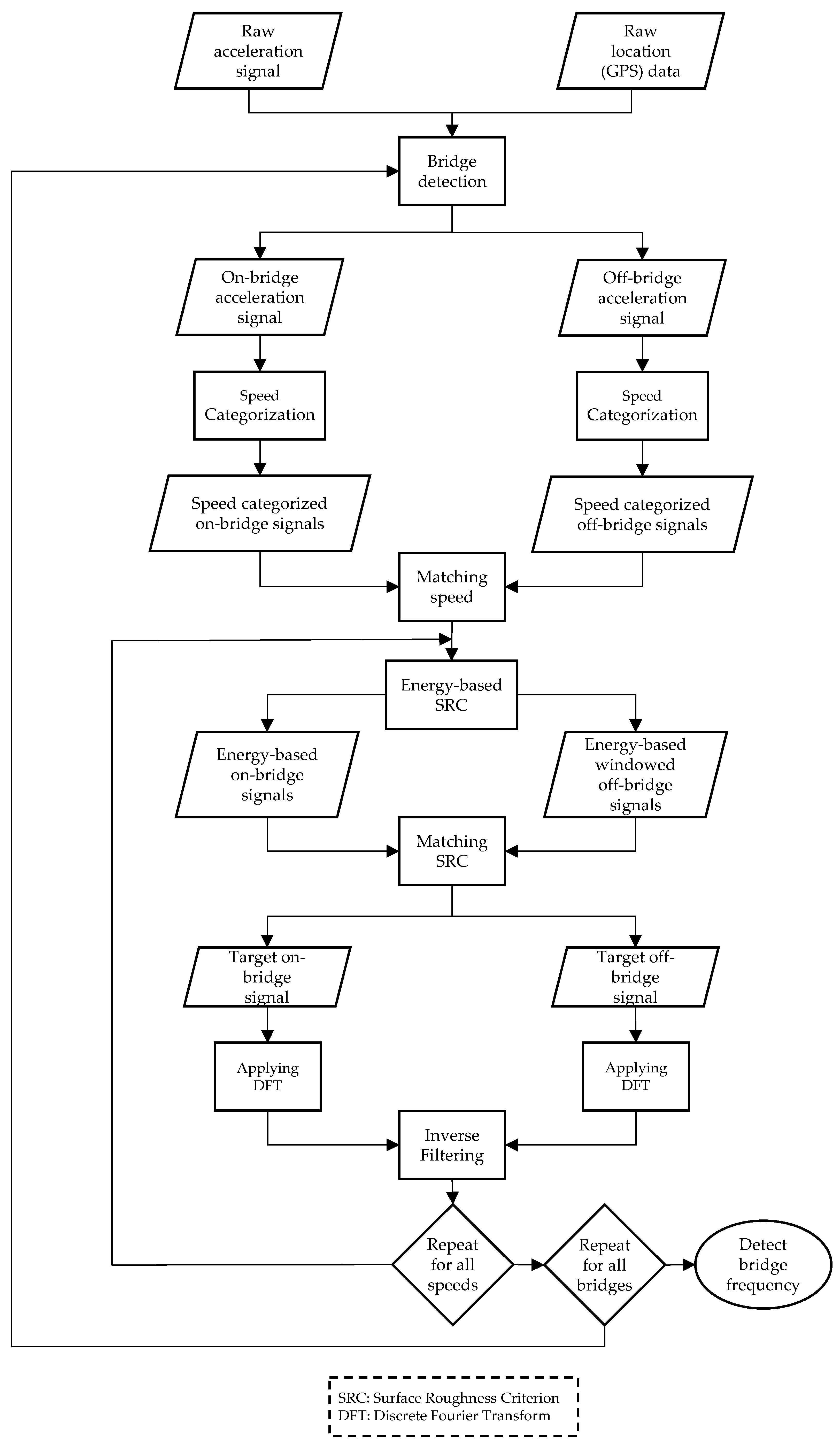
2. Methodology

In this section, first the concept of the vehicle-bridge coupled relationship as the main notion behind indirect bridge monitoring and the idea of inverse filtering will be explained. Afterwards, the process of data collection and analysis as well as the inverse filtering application will be discussed.

2.1. Concepts

2.1.1. Vehicle-Bridge Interaction

A moving vehicle acts as an exciter for a bridge structure. Meanwhile, the bridge itself affects the vehicle vibration as well. This system of vibration is governed through a coupled equation known as the vehicle-bridge interaction. One of the first studies on this concept was Yang and Yau [33]. They employed a simple 2D problem where the bridge was modeled using a beam model and a moving mass-spring system represented vehicle model. The resulting dynamic equation derived in that study clearly proves the interaction between the bridge and vehicle vibrations:

$$\{\begin{array}{c}\overline{m}(x)u_b^{″}(x,t)+E(x)I(x)u_b^{‴}(x,t)=c(x,t)\\ m_v{u}_v^{″}(t)+k_v\left[u_v(t)-u_b(x,t)\right]=0\end{array}.$$

(1)

In Equation (1), these parameters represent the features of the vehicle model: x as the position along the bridge, v as the speed, m_v and k_v as the mass and stiffness and u_v as the vertical displacement relative to the initial condition. The parameters representing bridge features are: m as the distributed mass per unit length, E as the elastic modulus, I as the moment of inertia of the section and u_b as the vertical displacement relative to the equilibrium position. In addition to these parameters, t represents the time, c is the contact force between the vehicle and the bridge and prime notation denotes the time-derivative function. In fact, this system of equations comprises governing dynamic equilibrium equations of the bridge and the vehicle, respectively. Equation (1) demonstrates that any solution for the vehicle vibration will have bridge dynamic characteristics as well and vice versa. As a result, the recorded vibrations of a vehicle moving over the bridge contains dynamic features of the bridge, which can be extracted through signal processing techniques. This notion was later investigated by many other studies [28,34] in the literature.

2.1.2. Inverse Filtering

The main idea of inverse filtering lies behind the fact that there are a few persistent sources in the signal mix that could be filtered out in order to capture the features of a transient source. This idea was first introduced in audio signal processing [35,36], which later expanded to image processing [37]. In terms of indirect bridge monitoring, vibrations recorded on a moving vehicle comprise many different sources including suspension system, engine vibrations and surface roughness, which are persistent during car travel. However, when the vehicle moves over a bridge, a new transient source, i.e., bridge vibration, is added to the recorded vehicle vibrations. As a result, any filter with the capability of suppressing all persistent vibrational features would then magnify the bridge features. In this study, the focus is on identifying the fundamental frequency of the bridge. The inverse filter is constructed using the acceleration signals recorded on the vehicle while moving off the bridge, i.e., off-bridge signals. These acceleration signals are transformed into the frequency domain and then the filter shape is defined using the inverse of this off-bridge spectrum using the equation below:

$$F[k]=\frac{1}{\overline{X}[k]}$$

(2)

where $\overline{X}$ denotes the magnitude spectrum of the discrete-time Fourier transform (DTFT) of the off-bridge acceleration signals and F represents inverse filter shape. Later, the filter will be applied to the recorded signal while the vehicle is moving over the bridge, i.e., an on-bridge signal, and the bridge frequency will be extracted from the resulting inverse filtered spectrum. The filtered spectrum will be calculated as follows:

$$Y_f[k]=F[k]Y[k]=\frac{Y[k]}{\overline{X}[k]}$$

(3)

In Equation (3), Y[k] and Y_f[k] denote the unfiltered and filtered on-bridge spectra, respectively. This process is illustrated in Figure 1. for a sample of real-life data collected from the Walterdale Bridge described in the following sections. In Figure 1a, the off-bridge spectrum and its constructed inverse filter shape are illustrated with black and blue curves, respectively, while Figure 1b represents the on-bridge spectrum and the inverse filtered spectrum through black and blue curves, respectively. Note that the fundamental frequency of the bridge is shown with the dashed red line. As seen, Figure 1a demonstrates that the inverse filter suppresses the frequencies with higher amplitudes in the off-bridge spectrum, representing the major frequencies with the vehicle-related sources while amplifying lower amplitudes, yielding a clearer detection of an external vibrational source. The successful performance of the filter in Figure 1b shows the advantage of employing an inverse filtering methodology for bridge frequency detection. However, many factors may affect the performance of the filter, which are discussed in more detail in the next sections.

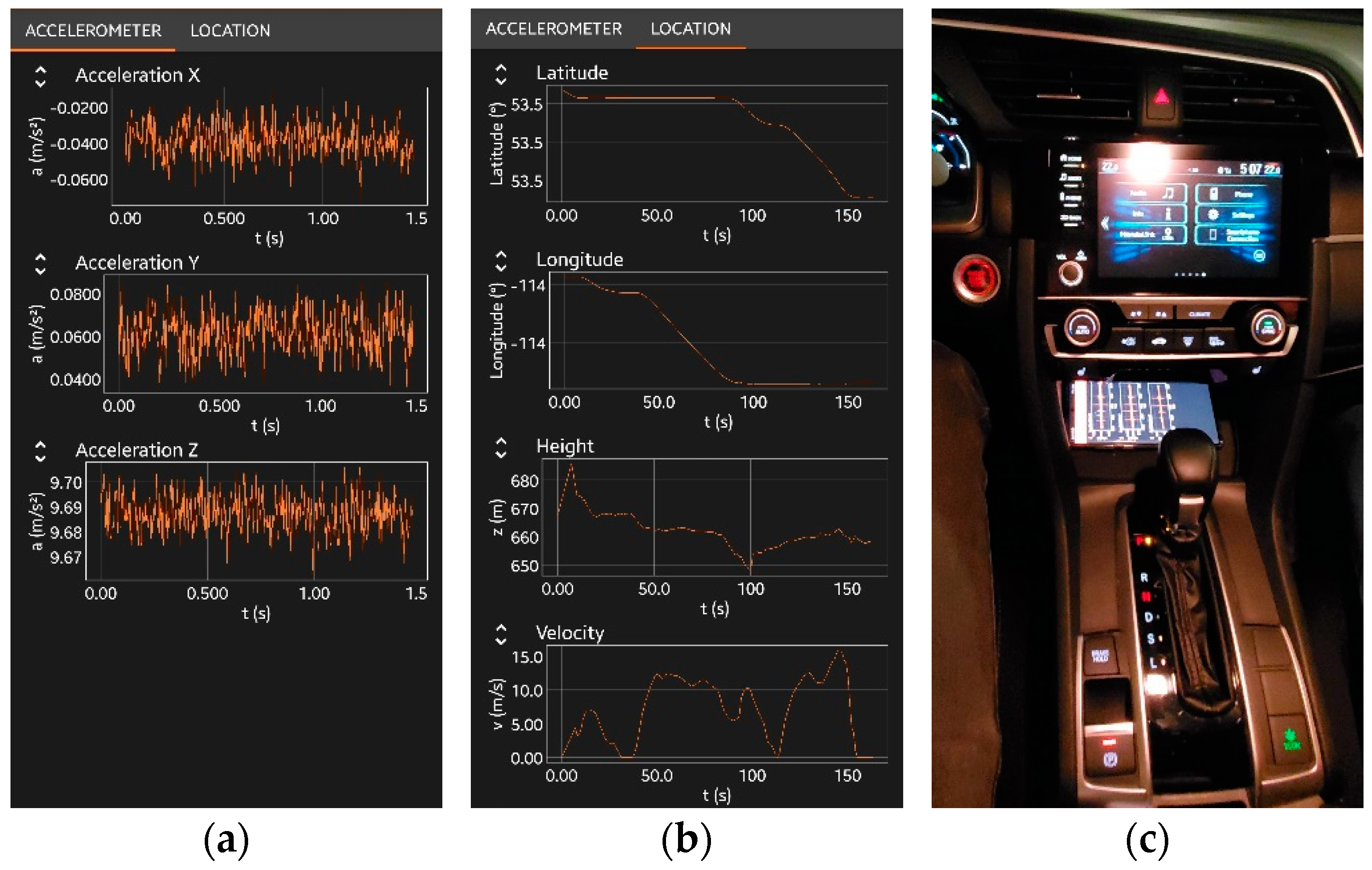
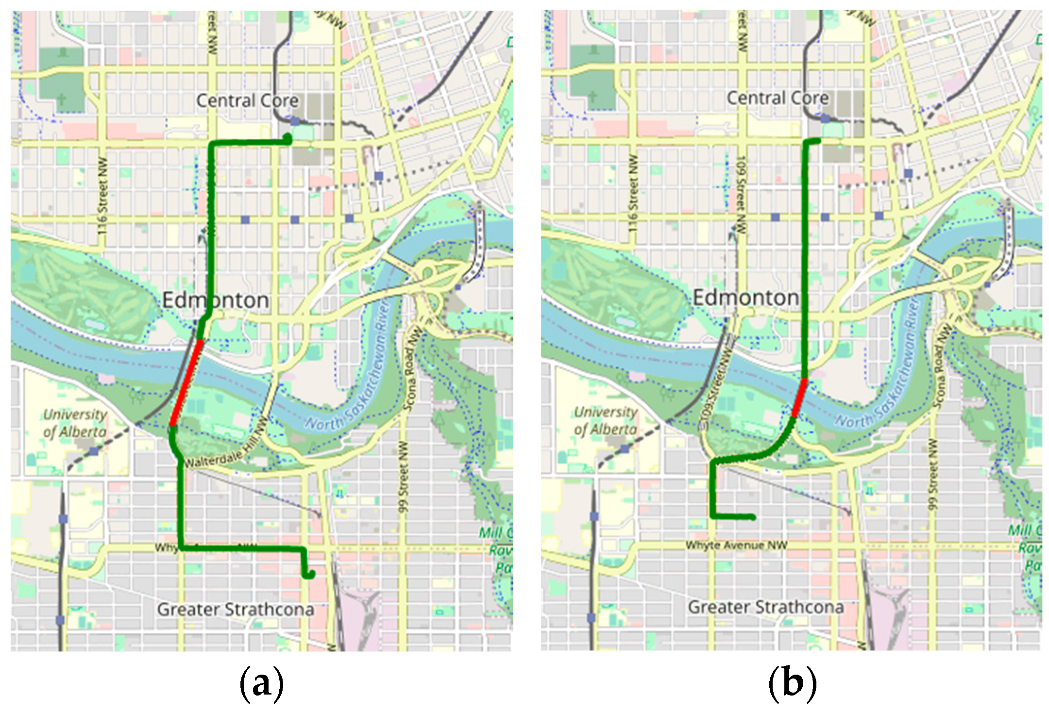
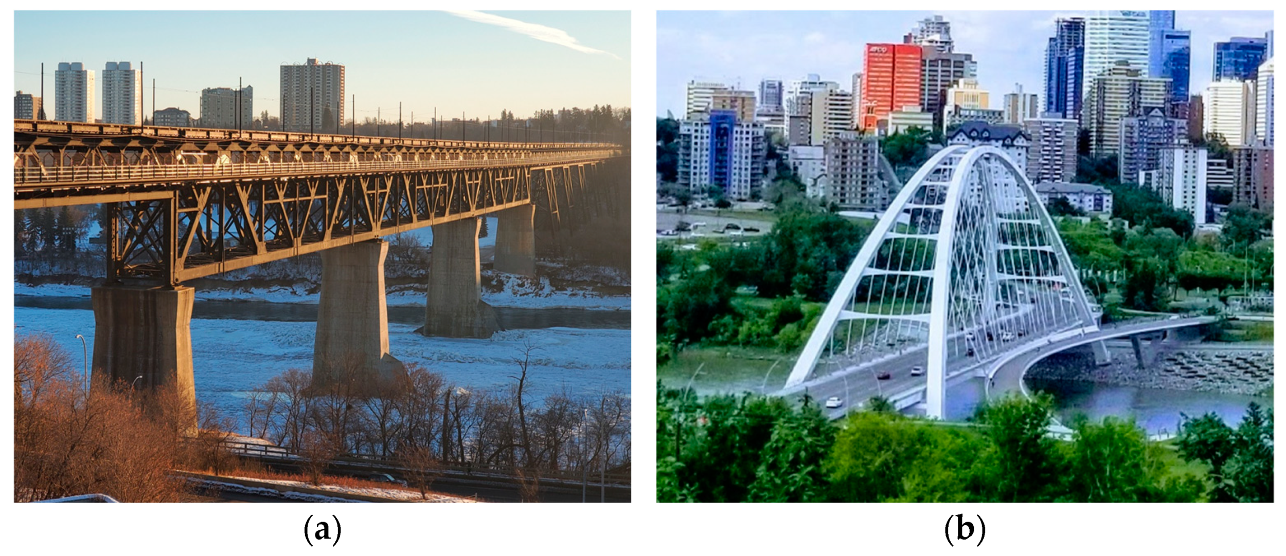
2.2. Data Collection

The required data for the proposed methodology consist of the vertical acceleration, as the main vibrational signal, and GPS, which will be used to determine the location of the vehicle and its speed. In this research, an academically developed smartphone application called phyphox [38], which was created at the 2nd Institute of Physics of the RWTH Aachen University, is employed. This application provides recordings of all of the smartphone sensors of which the accelerometer and GPS recordings are used in this study. The user interface of the application is shown in Figure 2a,b. In addition, the smartphone device used in this research is a Samsung Galaxy Note 10 Plus with the sampling frequency of 400 Hz for the accelerometer and 1 Hz for the GPS sensor and the vehicle where all of the recordings were conducted is a Honda Civic sedan. The placement of the smartphone inside the vehicle is also shown in Figure 2c.

2.3. Data Analysis

This section explains the procedure of the data analysis in the proposed methodology.

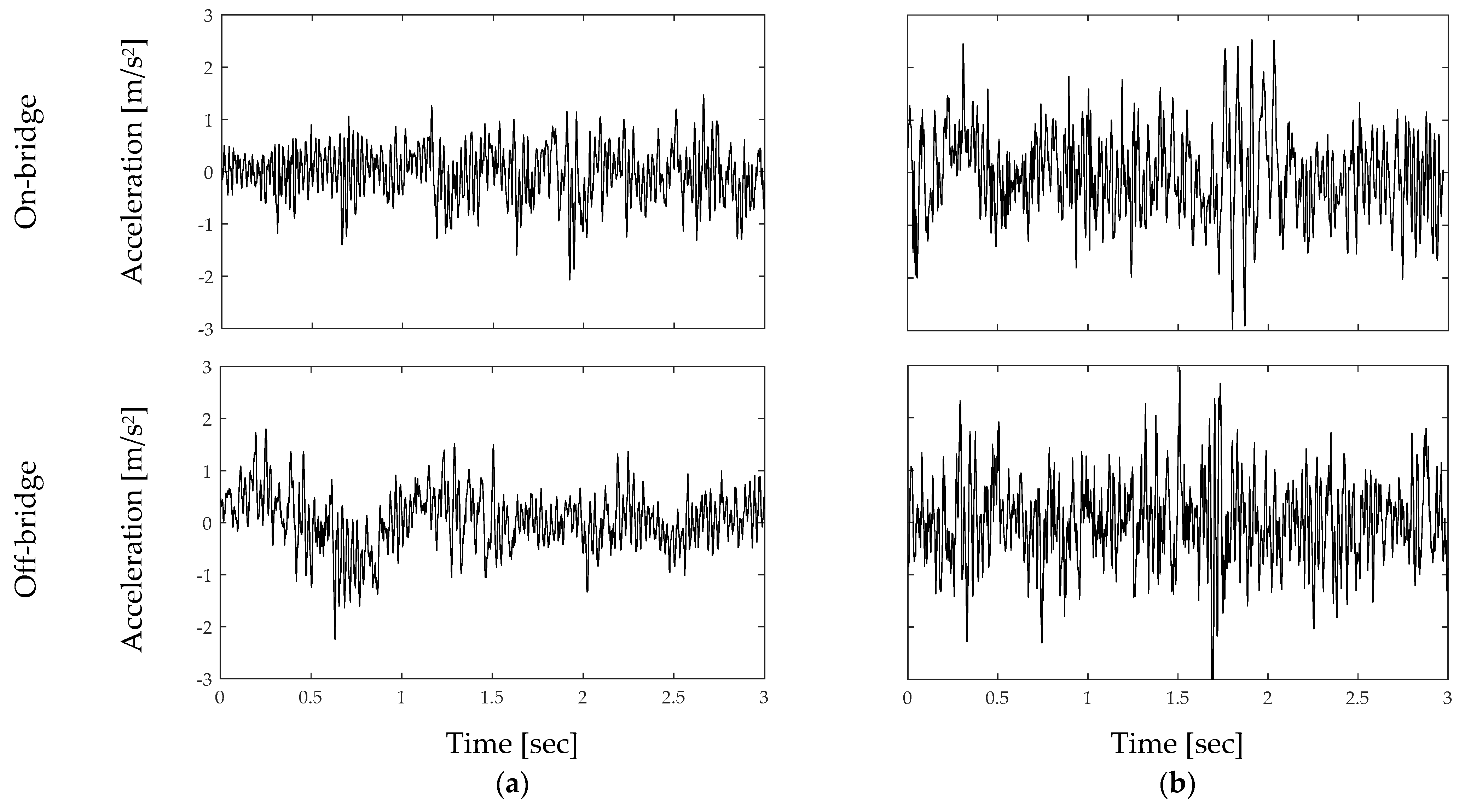
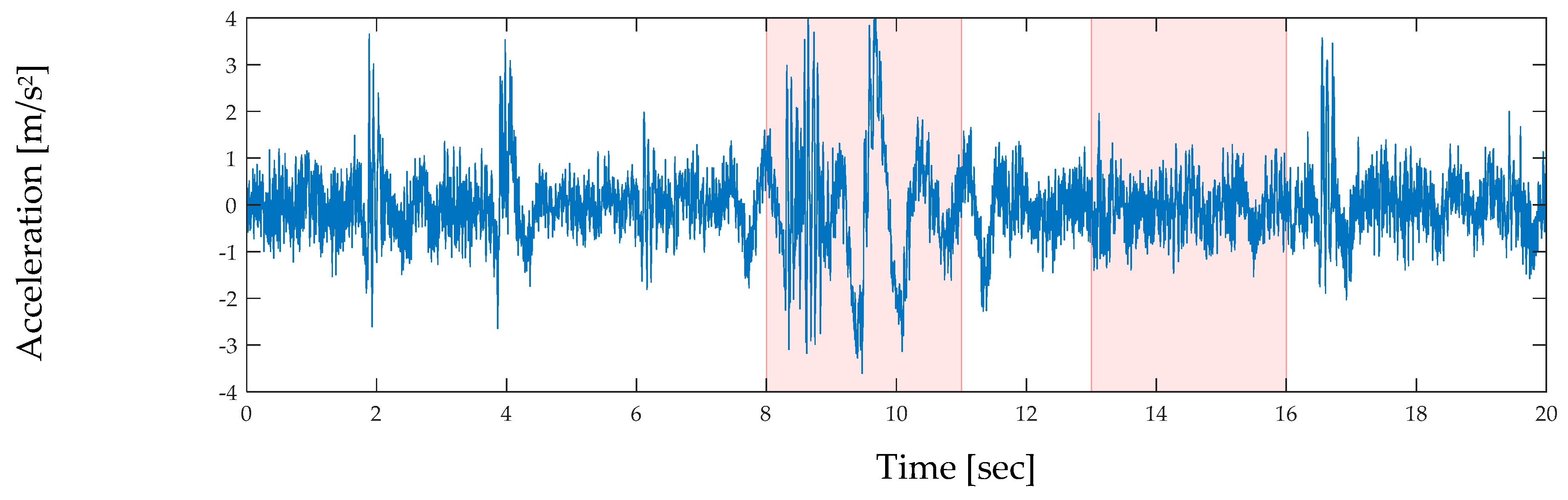
2.3.1. On-Bridge Data Extraction

The first step in the data analysis is to extract on-bridge segments of the acceleration signal. Based on the GPS coordinates of the start and end points of the target bridges, the time frames where the vehicle was moving on the bridge are determined. The corresponding on-bridge acceleration signals are then extracted according to those time frames. In Figure 3, one sample of GPS data and the captured bridges in Edmonton are shown on the map. The red line represents the target on-bridge segments and the green lines are the rest of the data, considered as off-bridge in the analysis.

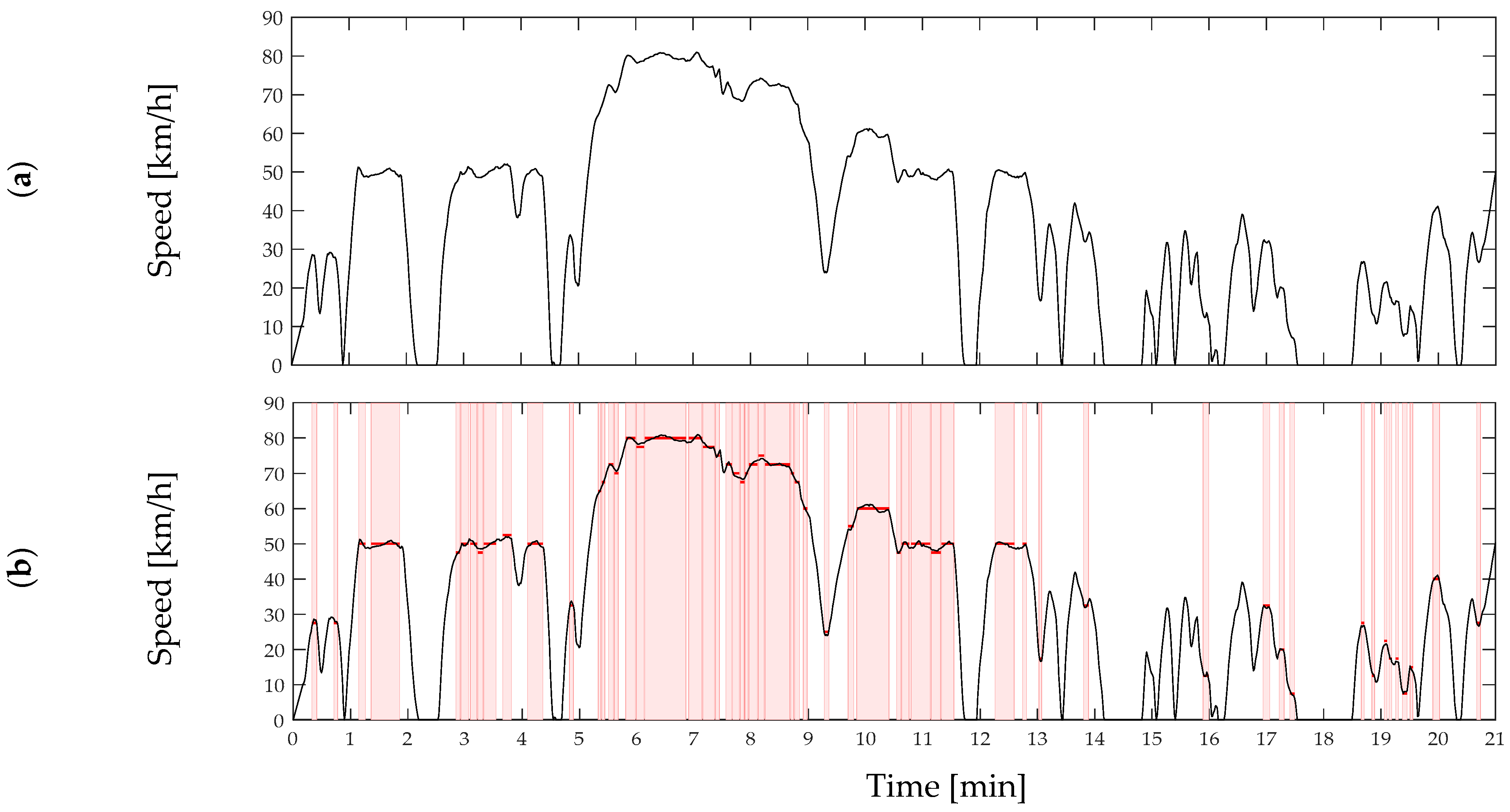
2.3.2. Speed Categorization

In order to account for the effect of the speed variations on the inverse filtering process, a database of the acceleration signals for different speeds is created. As the speed variation is continuous, the procedure of speed categorization is applied to create the database for discrete speed values. In the first step, the continuous values are changed to discrete speeds. In this study, equal speed bins of 2.5 km/h wide with the centers of multiples of 2.5 km/h are considered and the center values are assigned to all speeds that lie within the range of a bin. Furthermore, as the sampling frequency of the GPS sensor and hence that of the speed data is 1 Hz, i.e., one data point per second, there could be a chance of a speed change between the two consecutive data points. To account for this possibility, the minimum constant speed threshold is considered as the minimum consecutive time steps where the discretized speed is constant. Therefore, the possibility of a sudden speed change between the data points is reduced. The minimum constant speed threshold used in this study is three seconds. Hence, only the time frames where at least four consecutive discretized speed values are equal will be stored in the database. The process of speed categorization for a sample of speed data is illustrated in Figure 4. As seen, the shaded area in Figure 4b represents the selected constant speed segments, which are stored in the database to be later employed in the inverse filtering process.

2.3.3. Roughness Level Estimation

In addition to the effect of speed variations, the roughness level of the road has a significant effect on the performance of the inverse filtering method. In order to account for the variation in the roughness level, a roughness level criterion is proposed in this study, which is defined based on the average energy level of the vertical acceleration signal. It is expected that when a car is moving over a rough surface, the average energy level of the vertical acceleration would be higher in comparison with a smooth surface. In this study, the mean square of the acceleration values is employed as a measure of the energy level and therefore the surface roughness criterion (SRC). This criterion is later used for matching the off-bridge and on-bridge signals required for the inverse filtering application. This idea is presented in Figure 5, which consists of two columns. In each column, the upper plot shows the on-bridge acceleration signal recorded on the High Level Bridge and the lower one represents the corresponding off-bridge signal with a similar estimated roughness level, all recorded at the same speed of 50 km/h. In column (a), which represents a relatively low roughness level, the SRC is close to 0.3 (m/s²)² while this criterion is close to 0.64 (m/s²)² for column b representing a relatively high roughness level. As seen, employing the proposed SRC makes it possible to account for the effect of the surface roughness. The advantage of the SRC in increasing the performance of the inverse filter in terms of selecting the corresponding on-bridge and off-bridge signals will be discussed in more detail in the Discussion Section.

Unlike on-bridge acceleration data, which are limited due to the length of a bridge, there are more off-bridge data recorded in the database per each vehicle speed. Thus, instead of considering all speed categorized off-bridge data as one signal, different windows are considered in order to find the best matching surface roughness level. In this study, windows of three seconds long with a 25% overlap are considered, which are applied to the off-bridge database and the best matching SRC window is selected for the inverse filtering step. This process is illustrated in Figure 6 where a sample of off-bridge acceleration data is shown and two windows with a relatively large SRC difference are shown. As a result, based on the on-bridge data, the closest SRC, i.e., best matching roughness level, is selected for the inverse filtering process.

2.3.4. Inverse Filtering Application

In the final step, the inverse filtering technique will be applied to detect the bridge frequency. To this end, first the bridge detection is performed and all acceleration data are divided into on-bridge and off-bridge classes. All of the off-bridge acceleration signals will then go through the speed categorization process to extract constant speed acceleration signals and build the database of the off-bridge signals. Afterwards, the speed categorization of the on-bridge signals will be conducted. In the next step, for each constant speed segment of the on-bridge signals, the SRC will be calculated. The similar speed categorized segments of the off-bridge acceleration data are then recalled from the database and the SRC will be calculated for different windows of the signals and the off-bridge segment with the closest roughness level will be selected. If the difference between the on-bridge and off-bridge SRCs is more than 5%, that on-bridge segment will be dropped out of the process. In other words, if an on-bridge signal is recorded on a vehicle moving on a surface with a specific roughness level that is not previously experienced by the same vehicle during its off-bridge history, that on-bridge signal will not be suitable for the inverse filtering analysis and will be neglected. Finally, the corresponding on-bridge and off-bridge signals will be transformed to a frequency domain using a discrete Fourier transform and the inverse filtering technique will then be employed to capture the amplified bridge frequency. The flowchart of the proposed method is presented in Figure 7. The real-life result of the method for the two real-scale bridge cases will be discussed in the next section.

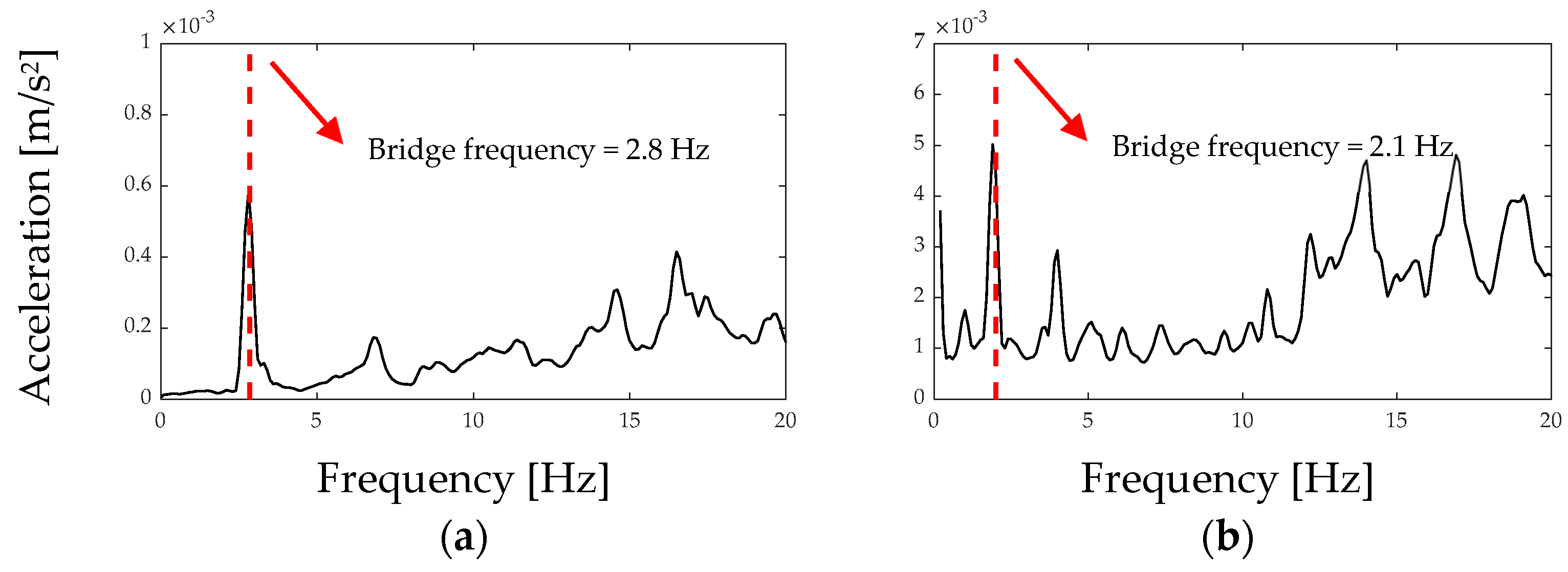
3. Results

In this section, the proposed methodology was tested in real-life practice for two different bridges in Edmonton, i.e., the High Level Bridge, a steel truss bridge with a length of 777 m built in 1913 and the Walterdale Bridge, a through-arch steel bridge with a total length of 214 m built in 2017, shown in Figure 8. Both bridges span over North Saskatchewan River that passes through the city. The fundamental frequencies of the bridges were captured through a frequency analysis of the recorded vibration under normal loading conditions. In that test, one minute long acceleration signals of bridge vibrations were recorded at one quarter, one third and one half of the length of the bridge using a standalone wireless accelerometer under the sampling frequency of 512 Hz and the first peak among all of those spectra was detected as the fundamental frequency. The identified frequencies were 2.8 Hz for the High Level Bridge and 2.1 Hz for the Walterdale Bridge. The spectra representing the middle point vibrations of the two bridges are shown in Figure 9. Note that these vibrational data were collected on a sunny summer day under the temperature of 20–26 °C. It is expected that the fundamental frequency of the bridges would slightly change in different environmental conditions, the effect of which is not in the scope of this study. However, these effects will be implemented in future studies through integrating artificial intelligence methods [39,40,41].

The inverse filtered spectra for the High Level Bridge and the Walterdale Bridge are presented in Figure 10 and Figure 11, respectively. Each figure consists of four plots organized in two rows representing different speed ranges of 40 to 50 and 50 to 60 km/h and two columns representing different surface roughness levels with the SRC ranges of 0 to 0.5 and 0.5 to 1 (m/s²)². In each plot, the original unfiltered on-bridge spectrum is illustrated with the blue color while the black color represents its inverse filtered spectrum. Note that the dashed red line denotes the fundamental frequency of the bridge. As seen, in most on-bridge cases, it was impossible to detect the bridge frequency with the raw unfiltered data due to the presence of vehicle vibrational features as well as the road roughness effect. However, the inverse filtering methodology together with the proposed speed database and surface roughness criterion was successful in detecting the fundamental frequency of the bridge. It should be noted that these data were collected on different days and the variations of environmental conditions, specifically the temperature, would cause a slight difference in the detected frequency of the bridge. It is expected that after applying the environmental adjustment methods to the proposed inverse filtering technique, these effective factors will also be addressed.

4. Discussion

Following the successful performance of the proposed methodology in the previous section, its effectiveness against two major factors in the indirect bridge frequency identification, i.e., vehicle speed and road roughness, is investigated in this section.

4.1. Effect of the Speed

As mentioned before, vehicle speed is one of the significant factors affecting the recorded vertical acceleration and its spectrum. To investigate this effect, a pair of off-bridge spectra recorded on a similar surface roughness level but at different speeds of 55 km/h and 52.5 km/h are presented in columns (a) and (b) of the first row of Figure 12, respectively. In addition, their corresponding inverse filter was designed and applied to a sample of on-bridge data recorded on the Walterdale Bridge in a vehicle with a speed of 55 km/h and their resulting inverse filtered spectra are presented in the second row of Figure 12. All of these spectra were recorded on a similar vehicle and under similar surface conditions with an SRC value of 0.7 (m/s²)². Note that the fundamental frequency of the bridge is shown with a dashed line. As seen, the slight difference between the vehicle speeds had a significant effect on the vibrational data and major irrelevant peaks occurred in the speed variant inverse filtered spectrum. This was due to the fact that major vibrational sources including the moving frequency of the vehicle and engine vibrations were all speed-dependent and a slight change in the speed of the vehicle changed the position of the major peaks in the spectrum, which was magnified in the inverse filtering process. This substantiates the fact that creating a speed-dependent database of the off-bridge signals is crucial in the successful performance of the inverse filtering for frequency identification of bridges.

4.2. Effect of the Surface Roughness

Surface roughness was the other important factor in the performance of the inverse filtering. The proposed energy-based SRC discussed in Section 2.3.3 played a significant role in the successful performance of the inverse filtering. In order to assess its influence, a pair of off-bridge spectra recorded under similar speeds but with different surfaces with SRCs of 0.7 (m/s²)² and 0.42 (m/s²)², respectively, are presented in columns (a) and (b) of the first row of Figure 13. In addition, their corresponding inverse filter was designed and applied to a sample of on-bridge data recorded on the Walterdale Bridge on a surface with an SRC of 0.7 (m/s²)² and their resulting inverse filtered spectra are presented in the second row of Figure 13. All of these spectra were recorded on a similar vehicle moving at a speed of 50 km/h. Note that the fundamental frequency of the bridge is shown with a dashed line. As seen, although the speed of the vehicle in both the on-bridge and off-bridge spectra was similar, the difference in the surface roughness levels made it impossible for the inverse filtering to extract the bridge frequency. In fact, the surface roughness was one of the sources that significantly affected the frequency content and hence the shape of the spectrum of the recorded acceleration signals. As a result, any comparison between the frequency content of on-bridge and off-bridge spectra needs to be under similar or close surface roughness conditions. The successful performance of the inverse filtering in the previous section demonstrated that the proposed SRC was efficient in detecting these similar surface conditions. Note that the results in Figure 13 demonstrated that the methodology worked properly for relatively high surface roughness levels as well although the vehicle features dominate vibrations over such surfaces making the bridge frequency identification challenging.

5. Conclusions

This paper proposed an enhanced inverse filtering methodology for the real-life applications of the drive-by frequency identification of bridges using smartphones through a new framework. Two major limitations of the previously proposed methodology were addressed here. First, it was proposed that through developing a database of off-bridge acceleration signals per different vehicle speeds, it would be possible to consider speed variations between off-bridge and on-bridge signals. In addition, a novel surface roughness criterion was defined based on the average energy level of the acceleration signal. Thus, the challenge of discrepancies between surface roughness levels of off-bridge and on-bridge conditions was also eliminated. The successful performance of the proposed approach for two real-scale bridges demonstrated the capability of the application for future bridge monitoring purposes. As all of the required data including the acceleration signals and the GPS data were collected from a smartphone, the implementation of the proposed method through a crowdsourced framework would significantly reduce the cost of monitoring a plethora of bridges in future smart cities. It should be noted that such methods can easily be extended to the embedded sensors in autonomous and connected vehicles.

It is worth noting that that the proposed methodology focused on detecting the fundamental frequency of the bridge only and further improvement is needed to detect higher modes of vibrations. Moreover, there were other important factors affecting the identification process specifically environmental effects such as temperature changes. These factors can drastically change the bridge frequency and should be considered for health monitoring purposes. In future studies and through further developments of the proposed methodology, a higher accuracy of frequency detection could be achieved, which is more suitable for damage detection purposes.

References

- Renkow, M.; Hoover, D. Commuting, migration, and rural-urban population dynamics. J. Reg. Sci. 2000, 40, 261–287. [Google Scholar] [CrossRef]
- Faturechi, R.; Miller-Hooks, E. Measuring the performance of transportation infrastructure systems in disasters: A comprehensive review. J. Infrastruct. Syst. 2015, 21, 04014025. [Google Scholar] [CrossRef]
- Serrano, W. Digital Systems in Smart City and Infrastructure: Digital as a Service. Smart Cities 2018, 1, 134–154. [Google Scholar] [CrossRef] [Green Version]
- Angelidou, M.; Psaltoglou, A.; Komninos, N.; Kakderi, C.; Tsarchopoulos, P.; Panori, A. Enhancing sustainable urban development through smart city applications. J. Sci. Technol. Policy Manag. 2018, 9, 146–169. [Google Scholar] [CrossRef]
- Silva, B.N.; Khan, M.; Han, K. Towards sustainable smart cities: A review of trends, architectures, components, and open challenges in smart cities. Sustain. Cities Soc. 2018, 38, 697–713. [Google Scholar] [CrossRef]
- Ham, H.; Kim, T.J.; Boyce, D. Assessment of economic impacts from unexpected events with an interregional commodity flow and multimodal transportation network model. Transp. Res. Part A Policy Pract. 2005, 39, 849–860. [Google Scholar] [CrossRef]
- Wilson, M.C. The impact of transportation disruptions on supply chain performance. Transp. Res. Part E Logist. Transp. Rev. 2007, 43, 295–320. [Google Scholar] [CrossRef]
- Canada Infrastructure Report Card. Monitoring the State of Canada’s Core Public Infrastructure; Canada Infrastructure Report Card: Ottawa, ON, Canada, 2019. [Google Scholar]
- Lucic, M.C.; Wan, X.; Ghazzai, H.; Massoud, Y. Leveraging Intelligent Transportation Systems and Smart Vehicles Using Crowdsourcing: An Overview. Smart Cities 2020, 3, 341–361. [Google Scholar] [CrossRef]
- Jan, B.; Farman, H.; Khan, M.; Talha, M.; Din, I.U. Designing a Smart Transportation System: An Internet of Things and Big Data Approach. IEEE Wirel. Commun. 2019, 26, 73–79. [Google Scholar] [CrossRef]
- Astarita, V.; Giofrè, V.P.; Guido, G.; Stefano, G.; Vitale, A. Mobile Computing for Disaster Emergency Management: Empirical Requirements Analysis for a Cooperative Crowdsourced System for Emergency Management Operation. Smart Cities 2020, 3, 31–47. [Google Scholar] [CrossRef] [Green Version]
- Costa, D.; Damasceno, A.; Silva, I. CitySpeed: A Crowdsensing-Based Integrated Platform for General-Purpose Monitoring of Vehicular Speeds in Smart Cities. Smart Cities 2019, 2, 46–65. [Google Scholar] [CrossRef] [Green Version]
- Händel, P.; Ohlsson, J.; Ohlsson, M.; Skog, I.; Nygren, E. Smartphone-based measurement systems for road vehicle traffic monitoring and usage-based insurance. IEEE Syst. J. 2014, 8, 1238–1248. [Google Scholar] [CrossRef] [Green Version]
- Gul, M.; Catbas, F.N. Structural health monitoring and damage assessment using a novel time series analysis methodology with sensor clustering. J. Sound Vib. 2011, 330, 1196–1210. [Google Scholar] [CrossRef]
- Noel, A.B.; Abdaoui, A.; Elfouly, T.; Ahmed, M.H.; Badawy, A.; Shehata, M.S. Structural Health Monitoring Using Wireless Sensor Networks: A Comprehensive Survey. IEEE Commun. Surv. Tutor. 2017, 19, 1403–1423. [Google Scholar] [CrossRef]
- Cho, S.; Jo, H.; Jang, S.; Park, J.; Jung, H.J.; Yun, C.B.; Spencer, B.F.; Seo, J.W. Structural health monitoring of a cable-stayed bridge using wireless smart sensor technology: Data analyses. Smart Struct. Syst. 2010, 6, 461–480. [Google Scholar] [CrossRef] [Green Version]
- Wenzel, H. Health Monitoring of Bridges; John Wiley & Sons: Hoboken, NJ, USA, 2008. [Google Scholar]
- Malekjafarian, A.; McGetrick, P.J.; Obrien, E.J. A review of indirect bridge monitoring using passing vehicles. Shock Vib. 2015, 2015, 286139. [Google Scholar] [CrossRef] [Green Version]
- Ozer, E.; Purasinghe, R.; Feng, M.Q. Multi-output modal identification of landmark suspension bridges with distributed smartphone data: Golden Gate Bridge. Struct. Control Health Monit. 2020, 27, 1–29. [Google Scholar] [CrossRef]
- Alavi, A.H.; Buttlar, W.G. An overview of smartphone technology for citizen-centered, real-time and scalable civil infrastructure monitoring. Future Gener. Comput. Syst. 2019, 93, 651–672. [Google Scholar] [CrossRef]
- Mei, Q.; Gül, M.; Shirzad-Ghaleroudkhani, N. Towards smart cities: Crowdsensing-based monitoring of transportation infrastructure using in-traffic vehicles. J. Civ. Struct. Health Monit. 2020, 10, 653–665. [Google Scholar] [CrossRef]
- Mei, Q.; Gül, M. A cost effective solution for pavement crack inspection using cameras and deep neural networks. Constr. Build. Mater. 2020, 256, 119397. [Google Scholar] [CrossRef]
- Mei, Q.; Gül, M. A crowdsourcing-based methodology using smartphones for bridge health monitoring. Struct. Health Monit. 2019, 18, 1602–1619. [Google Scholar] [CrossRef]
- Matarazzo, T.J.; Santi, P.; Pakzad, S.N.; Carter, K.; Ratti, C.; Moaveni, B.; Osgood, C.; Jacob, N. Crowdsensing Framework for Monitoring Bridge Vibrations Using Moving Smartphones. Proc. IEEE 2018, 106, 577–593. [Google Scholar] [CrossRef]
- Elhattab, A.; Uddin, N.; Obrien, E. Drive-by bridge frequency identification under operational roadway speeds employing frequency independent underdamped pinning stochastic resonance (FI-UPSR). Sensors 2018, 18, 4207. [Google Scholar] [CrossRef] [PubMed] [Green Version]
- Malekjafarian, A.; OBrien, E.J. On the use of a passing vehicle for the estimation of bridge mode shapes. J. Sound Vib. 2017, 397, 77–91. [Google Scholar] [CrossRef] [Green Version]
- Keenahan, J.; OBrien, E.J.; McGetrick, P.J.; Gonzalez, A. The use of a dynamic truck-trailer drive-by system to monitor bridge damping. Struct. Health Monit. 2014, 13, 143–157. [Google Scholar] [CrossRef] [Green Version]
- Hong, W.; Qin, Z.; Lv, K.; Fang, X. An indirect method for monitoring dynamic deflection of beam-like structures based on strain responses. Appl. Sci. 2018, 8, 811. [Google Scholar] [CrossRef] [Green Version]
- Catbas, F.N.; Aktan, A.E. Modal analysis as a bridge health monitoring tool. In Proceedings of the Structures Congress 2000: Advanced Technology in Structural Engineering, Philadelphia, PA, USA, 8–10 May 2000; Volume 103, pp. 1–10. [Google Scholar]
- Stiros, S.; Moschas, F. Rapid Decay of a Timber Footbridge and Changes in Its Modal Frequencies Derived from Multiannual Lateral Deflection Measurements. J. Bridge Eng. 2014, 19, 05014005. [Google Scholar] [CrossRef]
- Shirzad-Ghaleroudkhani, N.; Mei, Q.; Gül, M. Frequency Identification of Bridges Using Smartphones on Vehicles with Variable Features. J. Bridge Eng. 2020, 25, 04020041. [Google Scholar] [CrossRef]
- Shirzad-Ghaleroudkhani, N.; Gül, M. Inverse Filtering for Frequency Identification of Bridges Using Smartphones in Passing Vehicles: Fundamental Developments and Laboratory Verifications. Sensors 2020, 20, 1190. [Google Scholar] [CrossRef] [Green Version]
- Yang, Y.-B.; Yau, J.-D. Vehicle-Bridge Interaction Element for Dynamic Analysis. J. Struct. Eng. 1997, 123, 1512–1518. [Google Scholar] [CrossRef]
- Zhong, H.; Yang, M.; Jerry, Z. Dynamic responses of prestressed bridge and vehicle through bridge—Vehicle interaction analysis. Eng. Struct. 2015, 87, 116–125. [Google Scholar] [CrossRef]
- Wakita, H. Direct Estimation of the Vocal Tract Shape by Inverse Filtering of Acoustic Speech Waveforms. IEEE Trans. Audio Electroacoust. 1973, 21, 417–427. [Google Scholar] [CrossRef]
- Rothenberg, M. New Inverse-Filtering Technique for Deriving the Glottal Air Flow Waveform during Voicing. J. Acoust. Soc. Am. 1970, 48, 130. [Google Scholar] [CrossRef]
- Michailovich, O.; Tannenbaum, A. Blind deconvolution of medical ultrasound images: A parametric inverse filtering approach. IEEE Trans. Image Process. 2007, 16, 3005–3019. [Google Scholar] [CrossRef]
- Staacks, S.; Hütz, S.; Heinke, H.; Stampfer, C. Advanced tools for smartphone-based experiments: Phyphox. Phys. Educ. 2018, 53, 045009. [Google Scholar] [CrossRef] [Green Version]
- Zhang, H.; Gül, M.; Kostić, B. Eliminating Temperature Effects in Damage Detection for Civil Infrastructure Using Time Series Analysis and Autoassociative Neural Networks. J. Aerosp. Eng. 2019, 32, 04019001. [Google Scholar] [CrossRef]
- Gu, J.; Gul, M.; Wu, X. Damage detection under varying temperature using artificial neural networks. Struct. Control Health Monit. 2017, 24. [Google Scholar] [CrossRef]
- Kostić, B.; Gül, M. Vibration-Based Damage Detection of Bridges under Varying Temperature Effects Using Time-Series Analysis and Artificial Neural Networks. J. Bridge Eng. 2017, 22, 04017065. [Google Scholar] [CrossRef]
Publisher’s Note: MDPI stays neutral with regard to jurisdictional claims in published maps and institutional affiliations. |
© 2021 by the authors. Licensee MDPI, Basel, Switzerland. This article is an open access article distributed under the terms and conditions of the Creative Commons Attribution (CC BY) license (https://creativecommons.org/licenses/by/4.0/).
Share and Cite
Shirzad-Ghaleroudkhani, N.; Gül, M. An Enhanced Inverse Filtering Methodology for Drive-By Frequency Identification of Bridges Using Smartphones in Real-Life Conditions. Smart Cities 2021, 4, 499-513. https://0-doi-org.brum.beds.ac.uk/10.3390/smartcities4020026
Shirzad-Ghaleroudkhani N, Gül M. An Enhanced Inverse Filtering Methodology for Drive-By Frequency Identification of Bridges Using Smartphones in Real-Life Conditions. Smart Cities. 2021; 4(2):499-513. https://0-doi-org.brum.beds.ac.uk/10.3390/smartcities4020026
Chicago/Turabian StyleShirzad-Ghaleroudkhani, Nima, and Mustafa Gül. 2021. "An Enhanced Inverse Filtering Methodology for Drive-By Frequency Identification of Bridges Using Smartphones in Real-Life Conditions" Smart Cities 4, no. 2: 499-513. https://0-doi-org.brum.beds.ac.uk/10.3390/smartcities4020026