1. Introduction
Modeling lane changing is a challenging task that involves interactions of a vehicle and its immediate following and leading vehicle [
1,
2]. The existing lane change (
) algorithms (e.g., trajectory planning, maneuver planning algorithm) focus on maximizing the benefits to individual vehicles [
3,
4,
5,
6,
7,
8]. These algorithms require detailed microscopic traffic variables (i.e., relative speed and positions) of the surrounding subject vehicles, gaps between host and following and leading vehicles, which often depend not only on the behavior and movement of the surrounding vehicles, but also on macroscopic traffic dynamics [
2]. Hence, a simplified, yet reliable, macroscopic
prediction model that forecasts the probability of
occurrence in a relaxed cell (changes in time and space) is required [
1], moreso when the decision-making of lane changing is a critical link to drive the mission of connected autonomous vehicles in complex urban environments. Current research projects have focused on developing autonomous vehicle technologies to improve vehicle safety, particularly when performing its fundamental tasks, including car following, lane-keeping, and lane changing [
3,
4,
5,
6,
7,
8].
Studies related to macroscopic lane change (
) prediction have gained increasing attention in the macroscopic aspect of traffic simulation [
9,
10]. Efforts have been devoted to understanding various characteristics of
traffic based on the theoretical work of kinematic wave (KW), which ha viewed vehicular traffic as a continuous fluid flow and described the traffic dynamics by the changes in time and space [
11,
12,
13]. Among these macroscopic models, the cell transmission model (CTM)—a discretized version of the kinematic wave (LWR-KW)—model has been recognized as the simplest means to model the evolution of traffic dynamics and features [
14]. While fewer parameters are needed [
15], some limitation still exists, in which all the events related to
could not be explained fully in the current macroscopic traffic simulation models, partly due to lack of available data in a macroscopic form. Previous studies have considered the components of a lane change in developing the CTM model. Ref. [
16], e.g., assigned a fixed percentage of left-turn flow (i.e., 30%) when formulating the diverge movement to simulate oversaturated arterials. Their improved form of the CTM model, which introduced a novel conditional cell at the intersection, has enhanced the reliability of the CTM. However, some limitations still exist, where the assigned percentage of
at a fixed probability were not comprehensively taken into consideration and remain a question to be answered. Even though the percentage of
may be identified empirically from field observation or a defined lane changing rate, this does not mean it can be applied for any size of cells. These cells are influenced either by the surrounding traffic environment (i.e., speed and density between lanes) [
17,
18,
19,
20] or some unknown factors (i.e., driving attitude), which might affect the variance in the percentage of turning, or in a proper term, the probability of lane change. With the lack of comprehensive lane change in the rigid CTM model, the simulated traffic flow condition may not be accurately estimated with the actual traffic. Ref. [
21] have considered lane change in CTM, where they introduced
(i.e., the number of vehicles that wish to change lane at cell
, time step
) as a variable to determine the cell occupancies in the following time step. However, this variable has not been validated with actual data.
Due to its complex process, a macroscopic
algorithm that predicts the occurrence of
in a controlled zone, defined by space over time, was introduced [
17]. In a controlled space of a cell defined by space over time, the occurrence of lane change can be predicted in a logic binary form of either 0 (
or non-lane change) or 1 (
or lane change). In other words, each cell can capture the snapshot of the presence of
activities and the condition of the surrounding vehicles in the cell at any given stretch of road. Such discrete behavior of lane change has been evaluated in the previous studies using a statistical approach. One of the well-known statistical approaches is the binary logistic regression (BLR) technique. Few studies, however, have adopted the BLR to model the prediction of a lane change. Ref. [
17] have used the logistic regression to develop a lane change model-based, whereby macroscopic traffic variables (i.e., speed, density difference) are extracted and aggregated in a cell-based form. Their model predicted the probability of a lane change and showed statistically significant and non-linear relationships with macroscopic traffic variables. In their model, the occurrence of lane change was predicted at a 10-s time and 150 m length window. Ref. [
22] refined and further simplified the binary logistic lane change model suggested by [
17] by introducing the direction of the
and using lesser input variables. Ref. [
22] validated the proposed model with actual data and evaluated its performance using the area under the curve (
).
However, these studies had not considered the presence of multiple-lane change vehicles that is likely to occur simultaneously in this cell window [
17,
22]. Moreover, the expected probability of
will no longer be the same when the size of the cell windows changes with time step,
and cell length,
, which are affected by the surrounding traffic speed,
. It is known that the cell length,
is a product of speed,
, and time step
. The fact that the actual traffic speed varies over time gives us the reason why it is crucial to replace the conventional logistic
model with the dynamic properties considering the changes of cell sizes, thus making the model less rigid in predicting
.
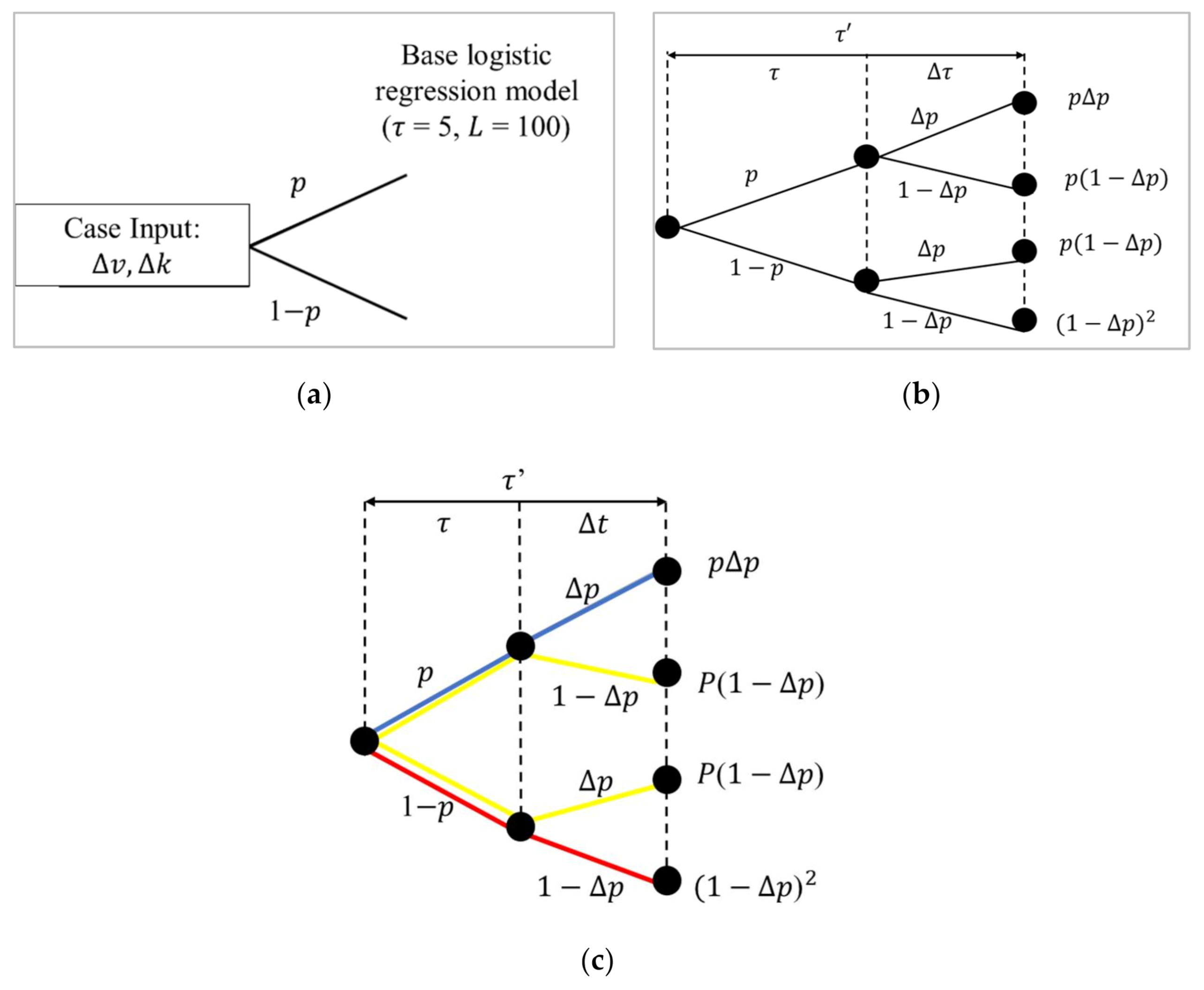
Aims of the Study
Indeed, abundant works focused on modeling behavior prediction and its improvement have been done in past research. However, some issues still need to be solved in emulating the complex behavior of lane change. A crucial drawback of current logistic regression lane change models is that they do not address the flexibility of the model in predicting lane change when the cell sizes, defined by space over time, change. Since the current logistic regression model only limits predicting the probability of from the binary response, the observations of two or more consecutive events are not possible using this regression approach.
Intending to overcome the aforementioned deficiencies, this study developed an improved version of the logistic model by proposed an event tree to expand the probability estimation of the conventional logistic regression for both single and multiple events of the lane change. Expanding the probability of with an event tree in the form of nodes and branches has the potential in dealing with the decision-making process for the issues as identified earlier. An event tree produces the probability outcome that is generated based on predetermined cell size. By tracing the event tree, one can observe the different outcomes on the probability of lane change based on any inputs of macroscopic traffic variables and the ability to predict lane change of any cell sizes while observing the events of single and multiple lane changes. Considering the limitations of the conventional logistic regression, none have yet attempted to expand this model using this method, which is worth exploring. Therefore, this study proposes a macroscopic prediction model to calculate the probability of occurrence based on an event tree approach.
The main work of this paper includes the following four parts: (1) developing a pre-defined event-based logistic regression model based on field data; (2) introducing the framework of the event tree, which expands upon a pre-defined logistic regression model; and (3) predicting the occurrence as zone sizes changes; and (4) evaluating the performance of the proposed model.
The remainder of the paper is organized as follows.
Section 2 introduces the basic terminology of the logistic regression model and the variables used in the study. The framework for the extended model based on the event tree approach is provided in
Section 3. The main work includes the following three parts: (1) developing a pre-defined
event-based logistic regression model; (2) introducing the framework of the event tree, which is expanded upon a base logistic regression model; and (3) predicting the
occurrence as zone sizes changes; and (4) evaluating the performance of the proposed model by presenting the empirical results.
Section 4 gives a brief description of the training data used for the regression model.
Section 5 describes the methods of evaluating the performance of the regression models. In
Section 6, results and discussion are provided, and the effectiveness of the extended model is validated and compared with the actual status of
at different conditions. Lastly, the conclusion of the paper is provided in
Section 7.
5. Performance Measures
From a theoretical aspect, extended the logistic regression lane change model using the branching of event trees has demonstrated (in the previous section) the possibility of the model to predict the probability of both single and multiple in any cell size. However, the improved model still needs validation with the actual data in order to be reliable at predicting the probability of .
With that in mind, the performance of the extended model is assessed by examining the discriminating power of classifying the agreement between the predictions and the actual outcomes. These classifications can be determined using a confusion matrix table that can further give specific performance measures, such as the true-positive rate, false-negative rate, true-negative rate, and the false-positive rate. Furthermore, predictive accuracy has also been widely used to assess the predictive capability of the logistic regression models. In this case, accuracy is the proportion of
and
that our models correctly classified. Thus, accuracy together with
was used to evaluate the performance of the tree-based logistic lane change models.
where
(true positive) and
(true negative) are the numbers of
events that are correctly classified, and
(false positive) and
(false negative) are the numbers of
events incorrectly classified.
The relationship between the true and false positives can also be depicted by a receiver operating characteristics (
) curve for visualization, organization, and selection of the classification model on the basis of their performance. To compare classification models, the performance measure of
can be reduced to a single number which is represented as the area under the
curve, abbreviated as
[
42]. In general, the bigger its
, the better the discriminative ability of a classification model, or in other words, the better is the overall performance of a model. Hence,
> 0.9 are considered outstanding,
between 0.8 and 0.9 are considered excellent,
between 0.7 and 0.8 are considered acceptable, and
between 0.6 and 0.7 are considered poor, non-discriminative if the
equals 0.5 [
43].
6. Results and Discussion
Following the need for a base model to be used as the root of the event tree, this section will first explore the NGSIM dataset by processing the data for different cell sizes in the search for the least multiple
events. After having a base model selected, the results will then compare the prediction of lane change between the event tree, its logistic regression, and the actual observations seen in the dataset. To see the reliability of the improved logistic regression model in predicting the lane change, the results will then present the model’s performance based on what has been discussed in
Section 5.
6.1. Selection of Base Model—Based on the Number of Observations
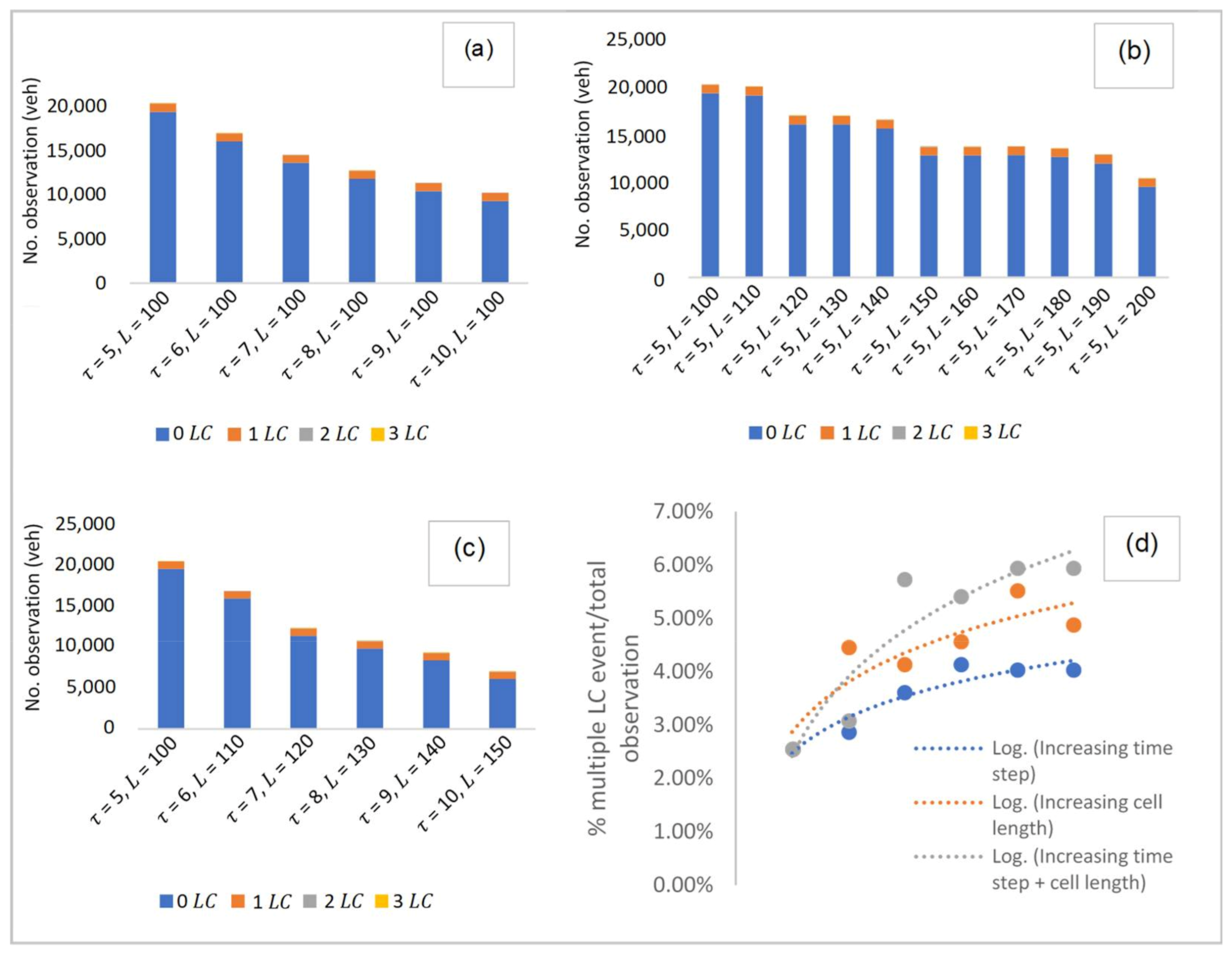
Several cases were explored in selecting the base model. As shown in
Figure 5, these cases were divided into: (i) observing at increasing time step in the same cell length, (ii) observing at increasing cell length for the same time step and, (iii) observing at increasing time step and cell length. Raw datasets from NGSIM were macroscopically processed based on each of the cases provided. In case (i), datasets were observed from
= 5 s, increasing at an interval of 1 s, up to
= 10 s in a fixed cell length of 100 m. Case (ii) observed datasets from cell length,
100 m, increasing up to
200 m at an interval of 10 m. Lastly, case (iii) observed the datasets whereby the time step and cell length are simultaneously increased at an interval of 1 s and 10 m, respectively, from
= 5 s,
100 m to
= 10 s,
150 m.
Here, a total number of observations for
and
events were found for each of these cases. In this figure (i.e.,
Figure 5), it can be observed that the number of
events is significantly much higher than the number of
events. Overall, a total of 943
events can be seen in the 45-minute collected within the discretionary lanes considered in the study area. Of these
events, some multiple events of
occurred simultaneously. However, when compared to the total number of
events, the events with multiple
constitute a relatively smaller percentage, i.e., approximately 2–4% for 2
events and <1% for 3
events. These are considered negligible when compared with the number of 1
events, which in turn, expect a low probability of
. Having known that a base model is required to be used as the root of the event tree for further prediction of multiple
events, the base model will thus be chosen, if possible, with the one with no multiple
events. In
Figure 5d, the number of multiple
events was compared for each case. It is observed that cell sizes with the smallest time step and cell length have the least multiple
events. In this case, the cell size of
= 5 s,
150 m were chosen as the ideal fit for the base model as it gives the lowest percentage of multiple
events at approximately 2%, which is considered negligible.
6.2. Prediction of —Comparing Different Approaches
In this section, a comparison is made to observe the probability of lane change predicted for different cell sizes. Specifically, the cell size considered were based on increasing time step and cell length ( 5, 100; 8, 130; 10, 150), which are then used to validate the predictions based on the following approaches:
Event tree for a specific cell size
Logistic regression processed for the respective cell size considered in (i). Note that different coefficients of the parameters are expected for different cell sizes.
Probability estimated from the actual status for the cell size considered in (i) and (ii), ( = number of observations/Total number of observations).
In all these, four separate quadrants observed among different input variables (i.e., speed and density difference) were also studied.
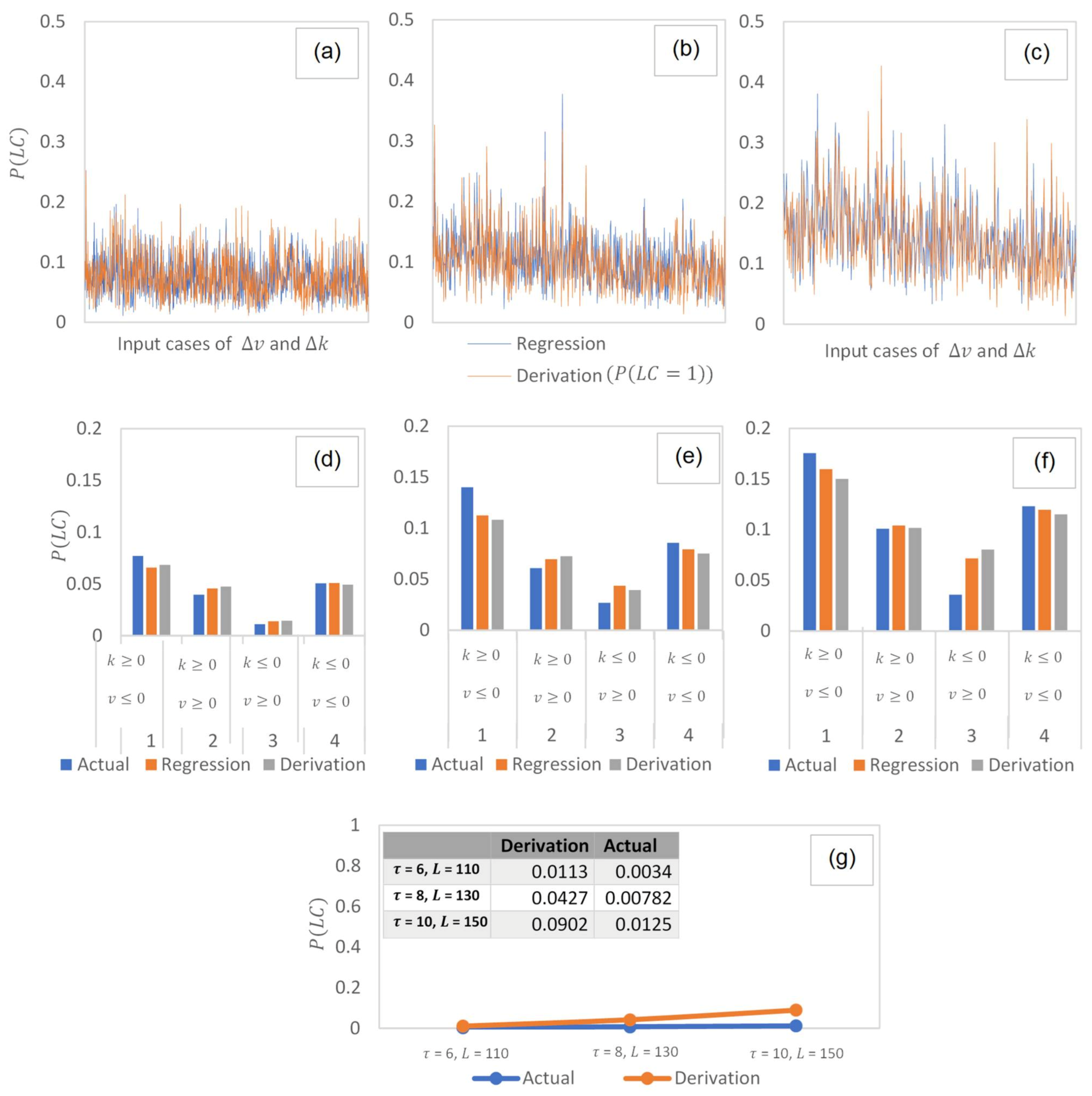
6.3. Observing Prediction of Single Events
Table 1 shows part of the results for the predicted probabilities in a cell size of
6,
110. Here, we wish to see whether there is a difference in the probability estimated between the event tree and the logistic regression for the respective cell size. To compare these approaches, an analysis of variance (ANOVA) was conducted on the probabilities estimated for the different input values obtained from data. The ANOVA tests whether the mean probability values are the same:
where
are the mean probability values at any approach
. Suppose a Type I error is controlled at
= 0.05, then
(0.95, 1, 1703) = 3.85 with 1 and 1703 as the degrees of freedom associated with the factor level and the error term of the given data. The decision rule is thus:
In this table, the -value = 0.11 > 0.05 and the crit = 3.85 > = 2.58. This shows that the null hypothesis, which states that all means are equal, cannot be rejected. In this case, the sample data (90% of the data used) is thus consistent with the hypothesis that population means are equal between groups. In other words, the predicted probability for the event tree does not differ much from the probabilities estimated from the logistic regression.
For
6,
110, approximately 65% of the
data have attained similar consistency between the two approaches (
-value = 0.11,
= 2.46), whereas 47% of the
data were found consistent at
10,
150 (
-value = 0.06,
= 3.67). Thus, as the cell size increases, lower accuracy is expected in predicting single lane change events. This can be explained by the presence of multiple-lane change events, which is much higher when the cell size increased (6% Multiple
events at
10,
150), see
Figure 6d.
Figure 6a–c provides the relative comparison of the probabilities estimated between the event tree and the logistic regression for (a)
6,
110, (b)
8,
130 and (c)
10,
150. For the
x-axis, the figure is plotted based on the outcomes of all the inputs (speed and density difference) found in the sample data. In these figures, it can also be clearly seen that the overall trends between the event tree and the logistic regression do not deviate much when predicting single observations of
.
6.4. Observing Prediction of Single Events at Different Input Variables
Figure 6d–f observes the ability of the extended model to predict the probabilities at different input variables. The dataset is further divided into four separate quadrants based on the positive and negative values of speed and density differences. In a plot of speed difference (
) against density difference (
), the four quadrants are defined as follow: (i) Quadrant 1 (
,
), (ii) Quadrant 2 (
,
), (iii) Quadrant 3 (
,
), and (iv) Quadrant 4 (
,
). A positive density difference means the origin lane has a higher density over the target lane, while a positive speed difference means that the origin lane has a higher speed over the target lane.
The comparison for each of the quadrants is made between (i) event tree, (ii) the logistic regression, and (iii) the actual in the dataset. For (iii), the probability is taken by dividing the number of observations by the total number of observations in the considered quadrants. Here, it is observed that all the three approaches (i), (ii), and (iii) have estimated probabilities that are close within the range of ±0.05 in each of the quadrants. The probabilities estimated were observed highest in Quadrant 1, where the origin lane is denser and at a speed lesser than the destination lane. This quadrant can also be categorized under the intention of discretionary lane change for the purpose of speed gain and travel time reduction.
6.5. Observing Prediction of Multiple Events
Figure 6g compares the prediction of multiple
events for different cell sizes. In this figure, the overall mean probability is taken for all the input cases found in the datasets of different cell sizes. It is observed that in a large sample size, the estimated average probability obtained for multiple
is <0.1. This is considerably smaller when observed in the field.
Comparing the average between the event tree with the actual observations, it is seen that the prediction of for the size at 6, 110, and 8, 130 are relatively close to each other. Further, a pairwise -test was conducted to compare the difference between the event tree with the actual observations. Results have confirmed no significant difference between the two samples (given -stat = 1.976 < critical two-tail = 4.303). Thus, the prediction for single and multiple observations of can successfully and accurately follow the pattern of actual data, which indicates the strong predicting ability of the event tree model.
6.6. Performance Measures of the Event Tree
In modeling the predictions of lane change, it is necessary to evaluate and assess the quality of the models for different cases. In this study, the models’ predictive accuracy,
curves, and
values were analyzed. Three evaluation statistics, namely, standard error, confidence interval at 95%, and significance level
, are included (see
Table 2 and
Table 3). The standard errors for each variable are reasonably small, confidence intervals are relatively narrow, and
-values are also small for all cases. All these results indicate a reasonable goodness-of-fit for the binary logistic regression with the dataset.
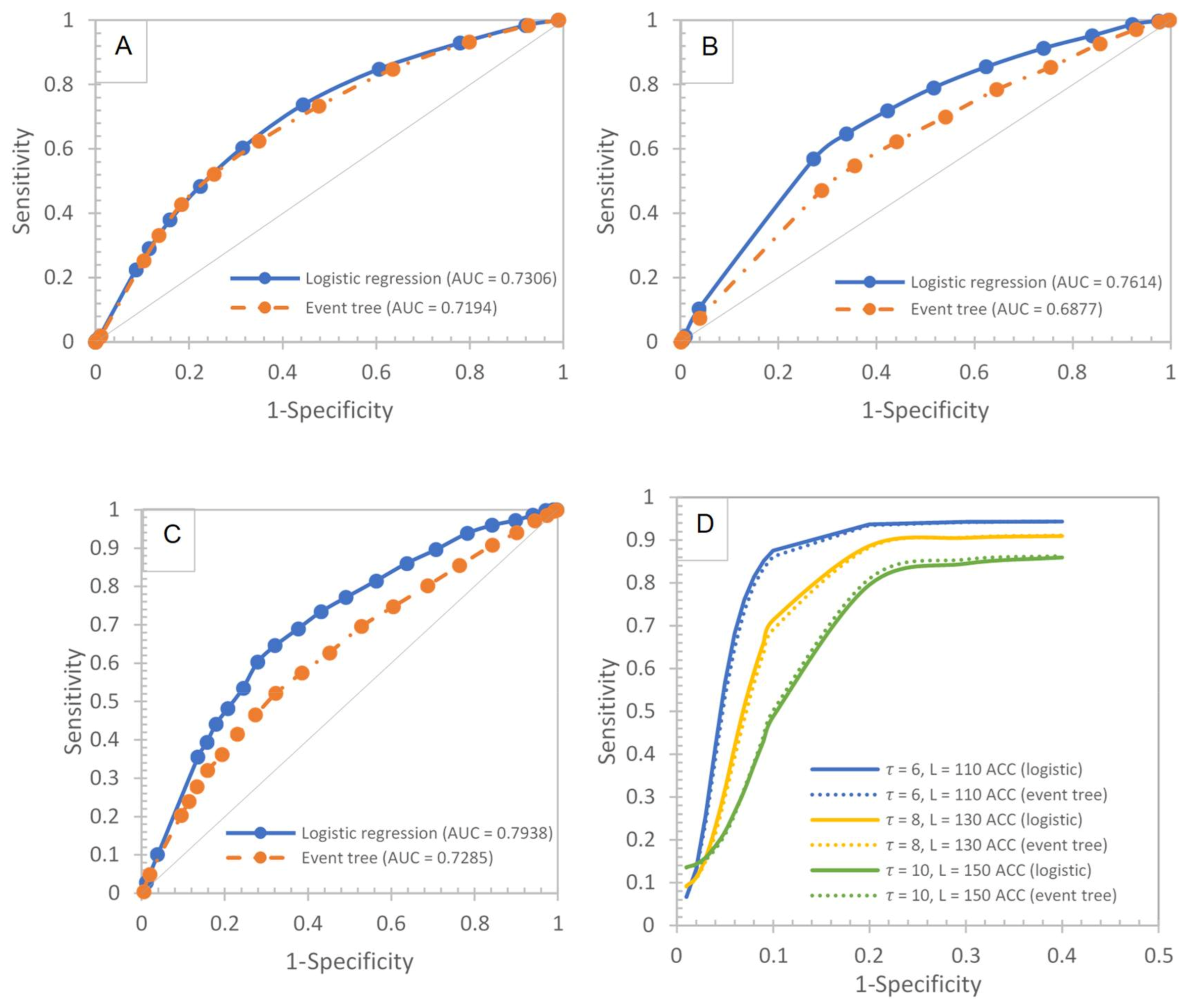
The prediction capabilities of the event tree were evaluated using validation, and results are shown in
Figure 7A–C. It can be seen that the logistic regression has a better prediction capability than the event tree with the highest accuracy value of 0.69 at the optimum cut-off point, an
value of 0.79. The other evaluation statistics for other cell sizes also indicate that the logistic regression exhibit reasonably good prediction capabilities. However, the capability of the event tree is not far off compared with the logistic regression, as they also have a numerically close prediction.
Finally, to compare the statistically significant difference between the logistic regression with the event tree, a pairwise comparison of these models was conducted on the performance figures. The null hypothesis is that there is no difference between the logistic regression and the event tree at the 95% significance level. An independent sample
-test and
-values are used to evaluate significant differences between them. When
-values exceed the critical values of
(4.30) and
-values are smaller than the significance level (0.05), the null hypothesis will be rejected. Therefore, the performances of the logistic regression with the event tree are notably different. The results of the Wilcoxon signed-rank test are shown in
Table 2. It can be seen that the performance of both the logistic regression and the event tree is not significantly different for all cases of increasing cell sizes (
-value = 0.12,
-value = 2.92).
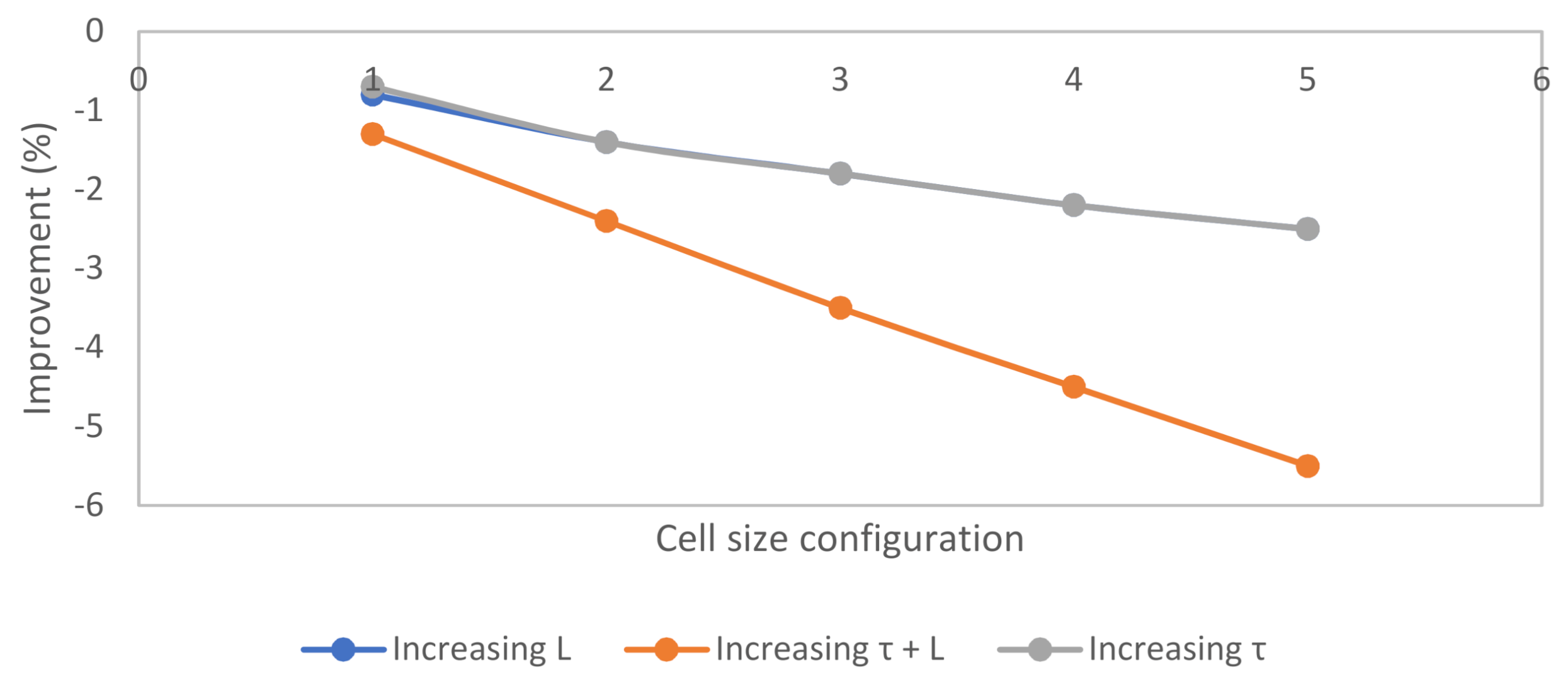
The probability estimated for both single and multiple
of the proposed event tree method was compared against the logistic regression for approximately 10,000 data points with the variable of varying speed and density differences from NGSIM. An overview of the result significantly shows an improvement in the accuracy up to 5.5% when comparing to the single
. The probabilities estimated considering multiple
, in general, generate smaller differences with the logistic regression model. It can also be observed that the accuracy improves as the cell configuration increases in its sizes from (1) to (5) at the cell size from
to
, as shown in
Figure 8. It should be noted that the negative % in the figure is an indication that shows multiple
being closer to regression than the single
. Considering multiple
, therefore, helps to improve the model accuracy for larger cell sizes.
The probability estimated for both single and multiple
of the proposed event tree method was compared against the logistic regression for approximately 10,000 data points with the variable of varying speed and density differences from NGSIM. An overview of the result significantly shows an improvement in the accuracy up to 5.5% when comparing to the single
. The probabilities estimated considering multiple
, in general, generate smaller differences with the logistic regression model. It can also be observed that the accuracy improves as the cell configuration increases in its sizes from (1) to (5) at the cell size from
to
, as shown in
Figure 8. It should be noted that the negative % in the figure is just an indication that shows multiple
being closer to regression than the single
. Considering multiple
, therefore, helps to improve the model accuracy for larger cell sizes.
7. Conclusions
In this paper, we have investigated the behavior of macroscopic prediction of lane change and proposed a relaxation method to improve the conventional logistic lane change model. Here, we have used an event tree method to expand the logistic regression from a base model that contains minimal observations of multiple lane changes. With speed and density as the input variable, the event tree is then extended according to a predetermined cell size defined by various time steps and cell length.
The reliability of the improved model is tested for the prediction of single and multiple events at different cell sizes and input variables. The findings from this study suggest that the use of the event tree can potentially replace the conventional logistic regression model in predicting lane change. Particularly, the prediction of the lane change based on the event tree approach has accurately followed the patterns of actual observation and the regression, which indicates the strong predicting ability of the event tree model.
However, results have shown that the conventional logistic regression still performs slightly better than the event tree in classifying the lane change and non-lane change events correctly. Regarding the the lower prediction capability of the event tree, they had managed to produce reasonable estimations when the conventional logistic regression models were not able to predict uncertainty due to changes in cell sizes and the presence of multiple-lane change events. The event tree is still acceptable for modeling the prediction of a lane change. It is generalized, simple, and easy to construct, thus lessen the amount of time to do regression numerously when the cell size changes.
In previous studies, researchers generally consider the model based on a restricted cell size that has yet to predict the presence of multiple-lane change events [
17]. In the same direction of modeling the lane change probabilities, [
44] also limit their interest to the scenario where each time interval is short as such, the lane change of each vehicle can only take place once. Hence, incorporating the event tree to extend the conventional logistic lane change model fills the gap of this study. The proposed method allows the relaxation to a different configuration of cell size, thus making the lane changing logic much simpler compared to the existing microscopic lane change models.
Finally, the model presented here can be extended to multiple vehicle classes by specifying class-specific lane changing probabilities. It is fully recognized that the reported results are based only on limited observation in a single location, which may not be sufficient to represent the general lane changing characteristics. Further studies to collect more data in different roadway layouts and identify some critical factors will be needed in the future. The improved lane change model will be integrated into the macroscopic Cell Transmission Model for traffic simulation with the consideration of multiple lane changes in future research. Analysis to be conducted comparing the outcomes of different Cell Transmission Models.


