Optimizing a Bi-Objective Mathematical Model for Minimizing Spraying Time and Drift Proportion

Abstract

The global agriculture sector faces many challenges in its mission to meet the increasing demand for food and fiber. Climate change, increasing population growth, emergence of crop diseases, damage to crops from rodents and critters, and shrinking farming land in some regions are among these challenges. Application of agrochemicals has proven to be an efficient answer to some of these challenges. However, the impacts of these products on human health and the environment combined with the increased requirement for sustainable farming requires the development of optimal spraying practices that would balance out all interests and concerns. In this paper, a mathematical model is developed to jointly minimize spraying time and drift losses. The obtained bi-objective mixed integer nonlinear programming model is solved for a case study example published in the crop protection literature. Optimal solutions are obtained using the weighted sum method and the epsilon-constraint approach. The results showed that valid and reasonable solutions can be obtained by selecting the appropriate combination of boom height, nozzle spacing, nozzle type, and tractor travel speed. Useful insights are obtained through various computational experiments.

1. Introduction

Sustainable agriculture aims at placing the agricultural inputs in such way to reduce the environmental degradation along with optimizing the operational efficiency and reduce the cost of operation. According to the US Farm Bill [1], “sustainable agriculture is an integrated system of plant and animal production practices having a site-specific application that will, over the long term: (a) satisfy human food and fiber needs; (b) enhance environmental quality; (c) make efficient use of non-renewable resources and on-farm resources and integrate appropriate natural biological cycles and controls; (d) sustain the economic viability of farm operations; and (e) enhance the quality of life for farmers and society as a whole”. In traditional farming, a blanket of treatment is applied throughout the field instead of treating only the problematic locations [2] without consideration for human health and contamination of the environment.

The increasing trend of applying agrochemicals in field crops is an integral part of the advance of agriculture. According to one study, in the United States, 3 million kg of agrochemicals costing 40 million US dollars are used annually [3,4]. Agrochemicals can save 45% of the world food supply by protecting crops from different insects and pests [5]. On other hand, this heavy use of agrochemicals has increased the risk of air, soil, and water pollution. During the application of these chemicals in the field, small spray particles move away from the intended areas (spray drift) and cause contamination [6]. Almost 30% of agricultural chemicals are wasted due to off-target spray drift [7,8]. This off-target spray drift could create health issues for animals and humans, damage nearby sensitive crops, and contaminate water sources and soils. However, Nuyttens [9] noted that reduction of the dosage of these chemicals may unfortunately reduce their effectiveness and could result in loss of money and chemicals. The increasing demand for food and fiber has forced farmers to apply agrochemicals. Therefore, spray drift became an important issue not only for public health but also for the scientific community. Spraying time is another important factor during the farm operation. In the modern agriculture world, timely execution of farming operations is required to ensure the efficiency of the activities by reducing activity durations, energy (fuel) use, labour hired, and overall cost (which is one pillar of sustainable agriculture) [10].

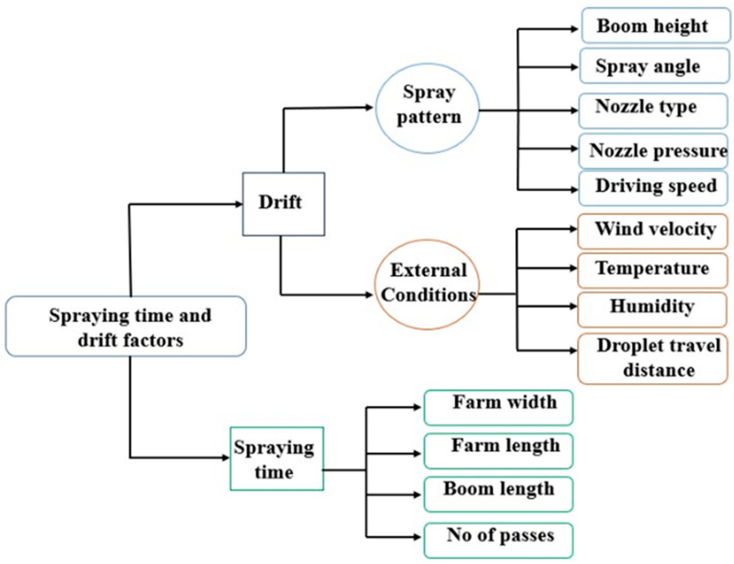
There are several factors which have direct influence on spray drift. These factors can be categorized into three major groups: (1) Sprayer related factors (boom height, driving speed, nozzle angle, nozzle pressure); (2) Weather conditions (temperature, humidity, wind velocity); (3) Crop conditions (crop type, crop height, crop stage) [9].

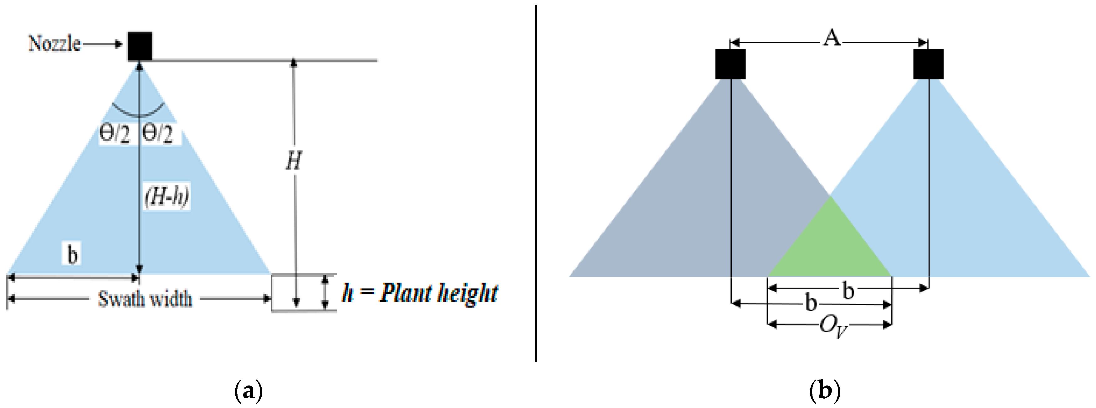
Different researchers studied the impact of these factors on spray drift individually. For example, [11,12,13,14] studied the impact of boom height on spray drift. These studies concluded that drift losses decreased by lowering the boom height. Drift losses can be decreased by 80% and 56% when the boom height is decreased from 70 cm to 30 cm and 50 cm to 30 cm respectively. Boom height has a significant impact on swath width (area covered by specific height and angle). Increasing the boom height increases the swath width and more area can be covered (which is good when crop canopy is fully developed) but on other hand, if the height is too high, then spray particles will be at more risk of moving with the wind and more drift losses will be expected [14].

The next important factor is tractor driving speed, which is directly linked with time of operation and has significant impact on spray drift [3,9,15,16,17] conducted experiments to see the impact of driving speed on spray drift and concluded that spray drift increased by 90% when the tractor speed increased from 7.0 km/h to 10 km/h. Nozzle type and its pressure are also important factors regarding the spray drift [3,18].

Al-Heidary [3] studied the influence of wind velocity on spray drift and concluded that as the wind velocity increases the drift losses increased. It is also recommended not to spray the field if wind velocity is 2.77 m/s or above [19]. Temperature and humidity had their own significance in spray drift study. High temperature and low humidity will increase the risk of spray drift due to high evaporation. High temperature and high the humidity will cause the suspension of spray particles in the air which will also contribute towards air contamination [3]. Crop type, crop height, and crop stage are also important consideration in spray drift study. Most of the studies investigate the impact of these factors on an individual basis.

Many researchers worked on the importance of drift by considering the sprayer related, weather related and crop related factors [3,11,12,13,14,15,16,17,18,19,20] but very few studies dealt with spraying time. Spraying time is another important factor, which is directly linked with drift losses and cost of spraying operation. Tobi [19] showed that farmers have no means to select efficient spraying speed. Their main goal is usually to finish as soon as possible given the labour and fuel costs. Thus, farmers usually opt for the highest speed possible without consideration for the fact that the selected speed could increase the hazardous effect of drift losses. Increased tractor speed will lead to the less spraying time but ultimately increases the drift. Drift losses increased by 51% when the tractor speed increased from 4.0 km/h to 8.0 km/h and 144% when tractor is operated at 16 km/h speed [19]. Therefore, there is a need for a trade-off between spraying time and drift.

2. Materials and Methods

2.1. Problem Definition

In this study, a bi-objective mathematical model is developed to find the optimal solution that minimizes both the spraying time and spraying drift proportion. Spraying time is affected by the tractor speed, farm length and width, boom length, and number of passes required. As covered in the literature review, multiple factors such as boom height, spray solution viscosity, spray angle, nozzle pressure, temperature and moisture content, and evaporation affect the drift proportion [3]. In this study, the following factors that affect spray drift will be considered: nozzle type, operating pressure, tractor speed, boom height, wind velocity, etc. This study deals with only these factors because these are the only ones for which drift proportion data was available from the field experiments ran by Nuyttens [20]. The proposed model can easily be extended to include all other factors enumerated by Al-Heidary [3], whenever full experimental data becomes available. It is also assumed that the factors considered in this study are independent and uncorrelated. This is reasonable as the data used to run the numerical experiments come from a field study that varied all these factors and corrected for correlation (See Nuyttens [20]). Figure 1 presents the drift causing factors along with the parameters that affect the spraying time. In general, drift amounts monotonously decrease as the measurement points get away from the point of application [9,20]. Therefore, in this study all drift measurements are considered to be made at a reference point set to a predetermined distance from the end of the field. Minimizing the drift amounts at the reference point is equivalent to minimizing the drift amounts at any other point or minimizing the total drift amounts.

The first objective function is the minimization of the spraying time. The second is the minimization of the spray drift proportion at a reference point. The optimization model aims at finding the best set up that will result in the best trade-offs between spraying time and drift generated.

This study focussed on the development of a mathematical model which provides a trade-off between spraying time and drift so that farmers can select the optimal settings for different parameters to reduce the spraying time along with drift. Our goals are:

• To develop a formula to calculate the spraying time by considering the farm width, farm length, boom length, number of passes and tractor speed.
• To develop the spray drift model by considering the external conditions and spray pattern related factors.
• To build a model to determine spray settings that trades off the travel time and drift.

2.2. Model Formulation

2.2.1. Notation (Indices and Parameters)

The notation (indices and parameters) used for the formulation of the bi-objective model are presented in nomenclature section of this manuscript.

2.2.2. Decision Variables

$$X_i^S=\{\begin{array}{cc}1,& iftractorspeedleveliisselected\\ 0,& otherwise\end{array}$$

$$X_j^H=\{\begin{array}{cc}1,& ifboom heightleveljisselected\\ 0,& otherwise\end{array}$$

$$X_n^N=\{\begin{array}{cc}1,& ifnozzle typenisselected\\ 0,& otherwise\end{array}$$

$$X_o^{\theta }=\{\begin{array}{cc}1,& if\mathrm{spraying}\mathrm{angle}\mathrm{level}oisselected\\ 0,& otherwise\end{array}$$

$$X_k^P=\{\begin{array}{cc}1,& ifpressure level k isselected\\ 0,& otherwise\end{array}$$

A = Nozzle spacing (multiples of attachment spacing: A = m × l. where m = 1, 2, ...)

θ = Selected spray angle in degrees (°) ($\theta ={\displaystyle \sum }_o{\theta }_o{X}_o^{\theta }$)

O_v = Overlapping of nozzle sheets (m) calculated as a function of A, H_j and θ.

2.3. Formulation of the Spraying Time

A field with a surface area of W_F × L_F (m²) is considered as pictured in Figure 2. A spraying tractor moves at a constant speed along the length (longest side) of the farm. The tractor is assumed to turn in semicircles when it reaches one end of the field to switch direction and start spraying in opposite direction without a gap in spray coverage as illustrated on Figure 2.

The total distance D traveled by the tractor is given by

$$D=c·W_F+\left(c-1\right)\pi ·\frac{L_B}{2}$$

(1)

For c, direction changes (passes), there are (c − 1) half circles to change direction. Distances traveled to and from the beginning or end of the field are not included in the optimization model.

The total spraying time is then obtained by dividing the total distance by the tractor speed S.

$$T_s=\frac{2{\mathrm{k}\mathrm{W}}_F{S}^{\prime }+\left(\mathrm{k}-1\right){\mathsf{\pi }\mathrm{L}}_{B}S}{2\mathrm{S}{S}^{\prime }}$$

(2)

where S is given by the selected speed level $S={\displaystyle \sum }_i{S}_i{X}_i^S$, and $S^{\prime }$ is the turning speed.

2.4. Formulation of the Drift Proportion

The assessment of drift is divided into two based on the involved factors according to Figure 1 under ‘external conditions’ (weather factors) and ‘operational aspects’ (sprayer related factors).

2.4.1. External Conditions

Humidity, temperature, wind velocity, and distance (travel distance of droplets from the outer nozzle) were considered as weather related factors. All these factors are considered as independent and non-correlated and combined in a single formula by Nuyttens [9] which constitutes a baseline drift (D_B) given by

D_B = d_d^−1.05(13.00 + 0.5V_3.25m + 0.4T − 1.74ζ_H2O)

(3)

where:

D_B = Fraction of applied spray which is lost during spraying and/or after application

d_d = Distance travelled by the spray particles in wind direction (m) (1 m, our study)

V_3.25m = Average wind velocity at height of 3.25 m above the ground level (m/s)

T = Average air temperature (°C)

ζ_H2O = Absolute humidity (weight of water vapours in grams per kg of dry air).

2.4.2. Operational or Spray Related Factors

The second component of the drift formulation relates to the drift proportion incurred by each of the spray related factors under consideration: speed of tractor (S_i), height of boom (H_j), nozzle pressure (P_k), and nozzle type (N_n). Using the field experiments carried out by Nuyttens et al., (2007b), a drift proportion value (${\Delta }_u^F$) is measured for each level u of each factor F. Illustrative examples of ${\Delta }_u^F$ are given in

Table 1. Relative drift proportion values for each level and each factor. Values are relative to the minimum value obtained by Nuyttens et al. 2017b.

	Nozzle Pressure			Height of Boom
K	Pk (bars)	${\Delta }_k^P$ (%)	j	Hj (m)	${\Delta }_j^H$ (%)
1	P1 = 2	0	1	H1 = 0.3	0
2	P2 = 3	3.5	2	H2 = 0.5	3
3	P3 = 4	6.5	3	H3 = 0.75
	Speed of tractor			Nozzle type	8
I	Si (km/h)	${\Delta }_i^S$ (%)	n	Nn	${\Delta }_n^N$ (%)
1	S1 = 4	0.6	1	N1 = F110 04	${\Delta }_n^N$ (%)
2	S2 = 6	0	2	N2 = F110 06	18.5
3	S3 = 8	2.7	3	N3 = F110 03	4
4	S4 = 10	2.1	4	N4 = F110 02	1.5
			5	N5 = LD110 02	2
			6	N6 = LD110 03	6.5
			7	N7 = LD110 04	3.5
					0

.

Thus, the total specific drift proportion (D_S) due to the four operational factors under consideration are given by

$$D_{\mathrm{S}}={{\displaystyle \sum }}_n{\Delta }_n^N{X}_n^N+{{\displaystyle \sum }}_k{\Delta }_k^P{X}_k^P+{{\displaystyle \sum }}_i{\Delta }_i^S{X}_i^S+{{\displaystyle \sum }}_j{\Delta }_j^H{X}_j^H$$

(4)

2.4.3. Total Drift Formulation

The total drift (T_d) is obtained as the sum of the baseline drift and specific drift.

T_d = D_B + D_B × D_S

(5)

$$T_d=D_{\mathrm{B}}(1+{{\displaystyle \sum }}_n{\Delta }_n^N{X}_n^N+{{\displaystyle \sum }}_k{\Delta }_k^P{X}_k^P+{{\displaystyle \sum }}_i{\Delta }_i^S{X}_i^S+{{\displaystyle \sum }}_j{\Delta }_j^H{X}_j^H)$$

(6)

From Equations (4) and (6), it can be seen that the baseline drift (D_B) is not affected by the decision variables ($X_n^N, X_k^P, X_i^S, X_j^H$), therefore this term will be dropped from the optimization model and only the specific drift proportion (D_S) will be optimized. The following subsection deals with the constraints that are included in the formulation.

2.5. Constraints: Levels Selection, Nozzle Spacing, and Overlapping of Spray Sheets

Of all the speed levels available, only one has to be selected for a given spray application, therefore, the following constraint is added to the formulation

$${\displaystyle \sum }_i{X}_i^S=1$$

(7)

Similarly, one and only one level has to be chosen for the nozzle type, the nozzle pressure, the boom height, and the spray angle. Thus, the following other constraints are obtained.

$${\displaystyle \sum }_n{X}_n^N=1$$

(8)

$${\displaystyle \sum }_k{X}_k^P=1$$

(9)

$${\displaystyle \sum }_j{X}_j^H=1$$

(10)

$${\displaystyle \sum }_o{X}_o^{\theta }=1$$

(11)

Uniform application of agrochemicals is an important quality requirement for spraying systems. Overlapping of spray sheets has significant impact on the uniformity of the spray applied to the crop canopy. Furthermore, nozzles spacing can be selected to control spray overlap depending on boom height. On a typical boom, there are by design locations where nozzles can be attached. For example, the operator can attach nozzles at each location (m = 1) or skip one location (m = 2) depending on the desired spacing $A=m\times l$. The constraint then is to select at least one location for the nozzle

$$m\ge 1$$

(12)

Once the nozzle spacing, spray angle and boom height are set, the spray sheet overlap can be calculated using the formulas developed below and based on the relationships depicted in Figure 3.

For a single nozzle (Figure 3a), the half swath width (b) is given by

$$b=\left(H-h\right)\tan \left(\frac{\theta }{2}\right)$$

where H is the boom height, h is the plant canopy height, $\theta ={\displaystyle \sum }_o{\theta }_o{X}_o^{\theta }$ and $H={\displaystyle \sum }_j{\Delta }_j^H{X}_j^H$.

The overlap between two consecutive spray sheets (Figure 3b) is given by

$$O_v=2b-A$$

$$O_v=2\left(H-h\right)\tan \left(\frac{\theta }{2}\right)-A$$

(13)

The overlap constraint, which is given as follows, ensures that the achieved overlap is between the minimum and maximum overlapping values set by the farmer or any other subject matter expert.

$$O_{min}\le O_v\le O_{max}$$

2.6. Bi-Objective Mathematical Model

The goal of the mathematical model developed in this paper is to investigate the trade-offs between the two-objective functions: spraying time (T_s called objective Z₁) and the specific drift proportion (D_s called objective Z₂). The full mathematical formulation is given below.

$$\mathrm{Minimize}{Z}_1=\frac{2k W_F{S}^{\prime }+\left(k-1\right)\mathsf{\pi }{L}_{B}S}{2\mathrm{S}{S}^{\prime }}$$

(14)

$$\mathrm{Minimize}{Z}_2 ={{\displaystyle \sum }}_n{\Delta }_n^N{\mathrm{N}}_n+{{\displaystyle \sum }}_k{\Delta }_k^P{\mathrm{P}}_k+{{\displaystyle \sum }}_n{\Delta }_i^S{\mathrm{S}}_i+{{\displaystyle \sum }}_j{\Delta }_j^H{\mathrm{H}}_j$$

(15)

Subject to

$${\displaystyle \sum }_i{X}_i^S=1$$

(16)

$${\displaystyle \sum }_n{X}_n^N=1$$

(17)

$${\displaystyle \sum }_k{X}_k^P=1$$

(18)

$${\displaystyle \sum }_j{X}_j^H=1$$

(19)

$${\displaystyle \sum }_o{X}_o^{\theta }=1$$

(20)

$$m\ge 1$$

(21)

$$O_{min}\le O_v\le O_{max}$$

(22)

$$X_i^S, X_n^N, X_k^P, X_j^H,X_o^{\theta }\in \left\{0,1\right\}$$

(23)

Constraint (23) states the binary variables and required m to be non-negative. The obtained formulation is a bi-objective mixed integer nonlinear programming model. The following section will present the approaches used to solve the mathematical model.

2.7. Solution Approaches

Both objective functions have different units: spraying time Z₁ is in hours (h) while drift proportion Z₂ is measured in percentage (%). To solve this kind of models, several approaches are available in the literature (see [21,22]). Here, we will use the weighted sums method and the ε-constraint (epsilon-constraint) method as done by Ghayebloo [22].

2.7.1. Weighted Sum Method

The weighted sum method combines both objective functions into a single function by assigning appropriate weights to each objective depending on the preference of the decision maker. Equation (24) shows the weighted sum formulation for our problem. The single objective function is normalized to 1 by dividing each objective function by its minimum possible value (Z_1min and Z_2min).

$$\mathrm{Minimize}Z =w\frac{Z_1}{Z_{1\min }}+\left(1-w\right)\frac{Z_2}{Z_{2\min }}$$

(24)

s.t.: Equations (16)–(23).

2.7.2. ε-Constraint Method

In this method, the multi-objective (bi-objective in our case) optimization problem is converted into single or mono objective optimization problem by retaining the objective function with highest priority (or preference) as the sole objective function and the other objective functions are rewritten and incorporated as constraints in the formulation. In this study, drift reduction is considered as the most important objective function and is retained as the sole objective function while spraying time is constrained to be less than or equal to a specific value $\epsilon$ ($Z_1\le \epsilon$). The ε-constraint formulation for our problem is shown below.

$$\mathrm{Minimize}Z =Z_2$$

(25)

s.t.: Equations (16)–(23).

$$Z_1\le \epsilon$$

3. Results and Discussion

In this section, a series of numerical experiments using parameter values from the field study conducted by Nuyttens [20] will be run and discussed to demonstrate the validity and applicability of the proposed mathematical model. Managerial insights will also be drawn to guide decision making by farmers and stakeholders. All experiments are run on an Intel™i5 3.4 GHz desktop computer with 16 GB of RAM running Windows 7™. The model is programmed in the optimization software MPL 5.0 (Maximal Software) and solved using the nonlinear solver LINGO Release 9.0 [23].

3.1. Experiment 1: Effects of Minimum Overlap in the Weighted Sums Method

In this experiment, seven different nozzle types (N_n), three different nozzle pressures (P_k), four different tractor driving speeds levels (S_i), and three different boom height levels (H_j) are used. The nozzle spacing was constant at l = 0.508 m while W_F = 0.4 km, L_F = 0.9 km and L_B = 0.02 km, h = 0.01 m.

Table 2. Results of the weighted sums method for minimum overlapping of 0, 0.4, and 0.95 m.

Case # 1: 0 m Minimum Overlap
w	0	0.1	0.2	0.3	0.4	0.5	0.6	0.7	0.8	0.9	1
Z	1.00	1.07	1.13	1.20	1.27	1.33	1.40	1.47	1.53	1.60	1.00
TS	2.20	2.20	2.20	2.20	2.20	2.20	2.20	2.20	2.20	2.20	1.32
H	0.3	0.3	0.3	0.3	0.3	0.3	0.3	0.3	0.3	0.3	0.3
OV	0.349	0.349	0.349	0.349	0.349	0.349	0.349	0.349	0.349	0.349	0.349
A	50.8	50.8	50.8	50.8	50.8	50.8	50.8	50.8	50.8	50.8	50.8
n	LD110.04	LD110.04	LD110.04	LD110.04	LD110.04	LD110.04	LD110.04	LD110.04	LD110.04	LD110.04	F110.02
P	2	2	2	2	2	2	2	2	2	2	2
s	6	6	6	6	6	6	6	6	6	6	10
Case # 2: 0.40 m Minimum Overlap
w	0	0.1	0.2	0.3	0.4	0.5	0.6	0.7	0.8	0.9	1
Z	1	1.07	1.13	1.20	1.27	1.33	1.28	1.21	1.14	1.07	1
TS	2.20	2.20	2.20	2.20	2.20	2.20	1.32	1.32	1.32	1.32	1.32
H	0.5	0.5	0.5	0.5	0.5	0.5	0.5	0.5	0.5	0.5	0.5
OV	0.9201	0.9201	0.9201	0.9201	0.9201	0.9201	0.9201	0.9201	0.9201	0.9201	0.9201
A	50.8	50.8	50.8	50.8	50.8	50.8	50.8	50.8	50.8	50.8	50.8
n	LD110.04	LD110.04	LD110.04	LD110.04	LD110.04	LD110.04	LD110.04	LD110.04	LD110.04	LD110.04	LD110.04
P	2	2	2	2	2	2	2	2	2	2	2
s	6	6	6	6	6	6	10	10	10	10	10
Case # 3: 0.95 m Minimum Overlap
w	0	0.1	0.2	0.3	0.4	0.5	0.6	0.7	0.8	0.9	1
Z	1	1.07	1.13	1.20	1.16	1.13	1.11	1.08	1.05	1.03	1
TS	2.20	2.20	2.20	2.20	1.32	1.32	1.32	1.32	1.32	1.32	1.32
H	0.75	0.75	0.75	0.75	0.75	0.75	0.75	0.75	0.75	0.75	0.75
OV	1.63	1.63	1.63	1.63	1.63	1.63	1.63	1.63	1.63	1.63	1.63
A	50.8	50.8	50.8	50.8	50.8	50.8	50.8	50.8	50.8	50.8	50.8
n	LD110.04	LD110.04	LD110.04	LD110.04	LD110.04	LD110.04	LD110.04	LD110.04	LD110.04	LD110.04	LD110.04
P	2	2	2	2	2	2	2	2	2	2	2
s	6	6	6	6	6	10	10	10	10	10	10

w = weight, Z = normalized objective function, T_S = spraying/travel time (h), A = nozzle spacing (m), H = boom height (m), O_V = overlap (m), n = nozzle type, P = nozzle pressure (bars), s = speed (km/h).

shows the results obtained for three values of the minimum overlap: 0, 0.40, and 0.95 m. The results are obtained by varying the values of the weight (w) from 0 to 1. When w = 0 then spraying time is not important and only drift reduction matters. Conversely when w = 1, then only minimizing spraying time matters. Intermediate values of w represent the preference expressed by the farmer or decision-maker between spraying time and drift reduction.

3.1.1. Weighted Sum Results for 0 m Overlapping (Case 1)

When w = 1, all the weight is given to spraying time and the value of the normalized objective function is 1. The optimal solution is then to set m = 1 (one nozzle at each position), use a flat fan nozzle F110 02 at a pressure of 2 bars with a boom height of 0.30 m and a tractor speed of 10 km/h, which will result in a spraying time of 1.32 h. Recall that when w = 1, drift reduction is not considered. These settings yield the fastest spraying in this study. This spray setting is very useful for row crops in their early stage when plants typically grow at a specific distance with no to little canopy. This setting is useful when applying the spray only on specific rows with less overlapping. This setting is useful only to finish the spraying operation very quickly or when the row distance equals the nozzle spacing. The boom height (0.3 m) will remain the same throughout this case due to less overlapping. It should be noted that running a 30 cm boom height at 10 km/h is only feasible for a relatively flat land as was the case for the experiments that generated the dataset being used here. On rougher terrain, the boom height will be raised from the optimal value to the nearest operationally viable height. Ideally, a dataset should be obtained for each type of terrain. Furthermore, it should be noted that any nozzle type other than F110 02 would work because drift reduction has a weight of 0. The result displayed in Table 2 is the first one that the mathematical model finds and reports. Other nozzle types are found on subsequent runs of the model and yield the same value of the objective function.

When the value of w is reduced to 0.9, the model suggests using a tractor speed of 6 km/h and nozzle LD 110 04 while maintaining the other parameters as before. As soon as drift reduction comes into play, the model reduces the traveling speed and uses a low drift nozzle to reduce drift. The same solution is obtained for the remaining values of w in Table 2. The model suggests that drift reduction is considered then there is a need to reduce tractor speed and to choose an appropriate nozzle.

3.1.2. Weighted Sum Results for 0.4 m Overlapping (Case 2)

In this case, the minimum overlap between spray sheets is increased from 0 to 0.40 m. Now changing the constraints of overlapping from 0 to 0.4 m. At w = 1, the optimal solution is: nozzle spacing of 0.508 m, nozzle type LD 110.04, pressure of 2 bars, tractor speed of 10 km/h, and boom height of 0.50 m. As expected, the boom height is increased to account for the need for more overlap. The switch from a 10 km/h to 6 km/h tractor speed occurs when w = 0.5 instead of 0.9 in Case 1. Raising the boom higher generates more drift than the change in speed so the model waits for the spraying time to be less important before reducing the speed to 6 km/h.

In this second case, the model also suggests the same nozzle type (LD110.04) for all values of w. The reason for this result is that the increase in drift due to the increased boom height is substantial, therefore the model suggests the nozzle with the lowest drift: LD110.04.

3.1.3. Weighted Sum Results for 0.95 m Overlapping (Case 3)

In this case, the minimum overlap between spray sheets is increased from 0.4 to 0.95 m. To achieve this required minimum overlap of 0.95 m, the model suggests raising the boom height to its highest position (0.75 m). All other settings remain the same as in Case 2. The switch from a 10 km/h to 6 km/h tractor speed occurs when w = 0.4 instead of 0.5 in Case 2. Increasing boom height will lead to the higher overlapping and increase the spray uniformity. This is useful when the crop canopy is fully-grown and covers the whole farm field. The spray sheet has maximum volume and velocity in its central part [24]. Therefore, higher overlap may be needed for uniform application [14,25,26].

Figure 4 shows a sensitivity analysis of the weight used in the normalized objective function. For low weight values (i.e., spraying time is less valuable), the normalized objective function is similar for all three minimum overlapping values. For high weight values (i.e., spraying time is more valuable), the normalized objective function is lowest for the highest minimum overlap. Across all weight values, the normalized objective function is lowest for the highest minimum overlap, meaning that this is the setting that gives the best trade-off between speed and drift regardless of the decision-maker’s preferences.

In the experiments above, the model almost exclusively selected the low drift nozzle LD110.04 yielding results with low variability in the spray settings. In the following experiment, the three low drift nozzles are removed from the data and only the seven standard flat fan nozzles F80.02, F80.03, F80.04, F80.06, F65.03, F65.04, and F65.06 are added to the existing four 110 degree flat fan nozzles. Using the observations from Al-Heidary [3] that drift losses were reduced by factors of 2 and 5 when going from 110-degree spray nozzle to 80- and 65-degree nozzles respectively, we estimated the drift proportions for the new nozzles based on the values available for the 110-degree nozzles. The corresponding drift proportions are given in

Table 3. Relative drift proportion values.

	Nozzle Type			Height of Boom
n	Nn	${\Delta }_{\mathit{n}}^{\mathit{N}}$ (%)	j	Hj (m)	${\Delta }_{\mathit{j}}^{\mathit{H}}$ (%)
1	N1 = F110 04	18	1	H1 = 0.30	0.0
2	N2 = F110 06	3.5	2	H2 = 0.35	0.8
3	N3 = F110 03	1.0	3	H3 = 0.40	1.5
4	N4 = F110 02	1.5	4	H4 = 0.45	2.3
5	N5 = F80 04	8.5	5	H5 = 0.50	3.0
6	N6 = F80 06	1.5	6	H6 = 0.55	4.0
7	N7 = F80 03	0.3	7	H7 = 0.60	5.0
8	N8 = F80 02	0.5	8	H8 = 0.65	6.5
9	N9 = F65 04	3.5	9	H9 = 0.75	8.0
10	N10 = F65 06	0.5
11	N11 = F65 03	0.0

. Furthermore, linear interpolation is used to find the drift proportions for boom heights at 35, 45, 55, and 65 cm. The results obtained are displayed in

Table 4. Results of the weighted sums method for minimum overlapping of 0, 0.1, 0.4 m.

Case # 4: 0 m Minimum Overlap
w	0	0.2	0.4	0.6	0.8	1
Z	1.00	1.13	1.27	1.40	1.53	1.00
TS	2.20	2.20	2.20	2.20	2.20	1.32
H	0.30	0.30	0.30	0.30	0.30	0.35
OV	0.055	0.055	0.055	0.055	0.055	0.02
A	0.1	0.1	0.1	0.1	0.1	0.4
n	F65.03	F65.03	F65.03	F65.03	F65.03	F110.04
s	6	6	6	6	6	10
Case # 5: 0.1 m minimum overlap
w	0	0.2	0.4	0.6	0.8	1
Z	1	1.13	1.27	1.4	1.53	1
TS	2.202	2.202	2.202	2.202	2.202	1.3212
H	0.3	0.3	0.3	0.3	0.3	0.75
OV	0.136	0.136	0.136	0.136	0.136	0.157
A	0.2	0.2	0.2	0.2	0.2	1.7
n	F80.03	F80.03	F80.03	F80.03	F80.03	F110.04
s	6	6	6	6	6	10
Case # 6: 0.4 m minimum overlap
w	0	0.2	0.4	0.6	0.8	1
Z	1.00	1.13	1.27	1.28	1.14	1.00
TS	2.202	2.202	2.202	1.321	1.321	1.321
H	0.5	0.5	0.5	0.5	0.5	0.75
OV	0.5	0.5	0.5	0.5	0.5	0.86
A	0.5	0.5	0.5	0.5	0.5	1
n	F110.03	F110.03	F110.03	F110.03	F110.03	F110.04
s	6	6	6	10	10	10

w = weight, Z = normalized objective function, T_S = spraying/travel time (h), A = nozzle spacing (m), H = boom height (m), O_V = overlap (m), n = nozzle type, s = speed (km/h).

for minimum overlap values of 0, 0.1, and 0.4 m and l = 10 cm.

The results in Table 4 show how the model moves from flat fan nozzle with the smallest top spray angle (65°) (Figure 5) when there is no overlap required to the medium spray angle (80°) (Figure 6) and finally to the highest spray angle (110°) (Figure 7) when high overlap is required. Similar behaviour is seen with the boom height. Trade-offs between speed and drift minimization appear in Case #6 at w = 0.6.

3.2. Trade-Off between Drift Reduction and Spraying Time Using the ε-Constraint Method

In the epsilon constraint model, drift minimization is retained as the sole objective function and spraying time is constrained to be less than or equal to a specific value ε ($Z_1\le \epsilon$).

Table 5. Results obtained with the ε-constraint method.

	Ovmin = 0.0 m			Ovmin = 0.4 m
Epsilon (h)	3.0	2.0	1.0	3.0	2.0	1.0
Z2	0.00	2.1	Infeasible	3.00	5.1	Infeasible
TS	2.20	1.32		2.20	1.32
H	0.30	0.30		0.50	0.50
OV	0.35	0.35		0.92	0.92
A	0.508	0.508		0.508	0.508
n	LD110.04	LD110.04		LD110.04	LD110.04
P	2	2		2	2
s	6	10		6	10

Z₂ = normalized objective function, T_S = spraying/travel time (h), A = nozzle Spacing (m), H = boom height (m), O_V = overlap (m), n = nozzle type, P = nozzle pressure (psi), s = speed (km/h).

presents the results obtained with the epsilon-constraint method with the dataset with seven nozzles used at the beginning of Section 3.1 above and for three values of ε: 1, 2, 3 h.

The maximum speed available is 10 km/h which allows to spray the farm in 1.32 h. Thus, the model is infeasible when $\epsilon =1$. When the spraying time is constrained to be equal or less than 2 h, the speed of 10 km/h is chosen with boom heights of 0.3 m and 0.5 m for minimum overlaps of 0 and 0.4 m, respectively. When $\epsilon =3,$ the travel speed is reduced to 6 km/h which yields the lowest drift proportion values.

The above results show that the proposed mathematical model is capable of selecting the appropriate operating configuration given the farmer’s preference level between minimizing drift losses and reducing spraying time. The parameters used in our numerical experiments are extracted from the field study conducted by Nuyttens [20], which involved 27 separate experiments. Thus, the number of combinations of settings that the mathematical model can choose from is limited resulting in low variation between solutions. However, these solutions are reasonable and valid: all selections made are explained above. Given the low computation times observed and the known efficiency of mathematical optimization, it is reasonable to assume that the model would easily run on larger datasets.

4. Conclusions

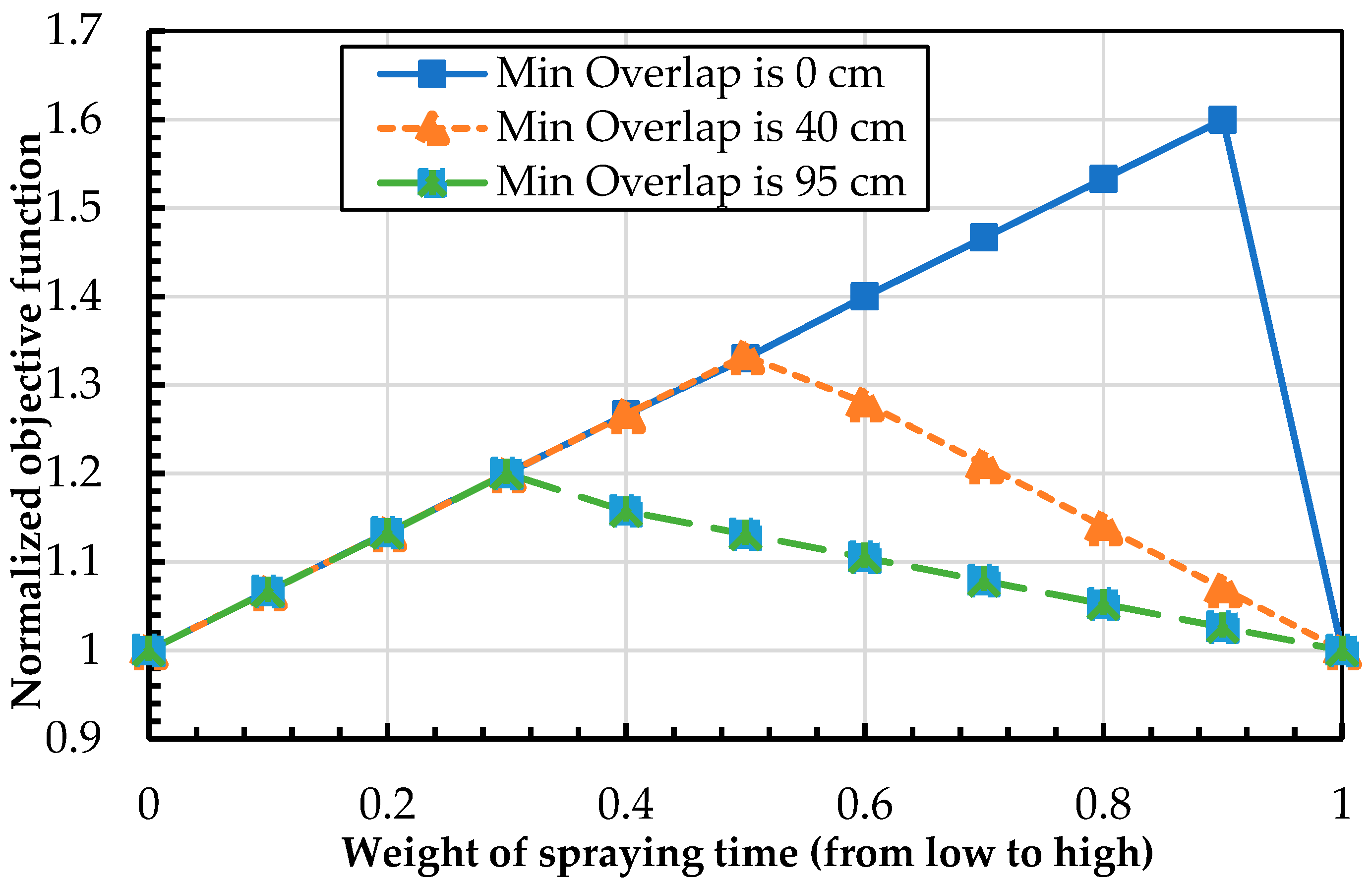
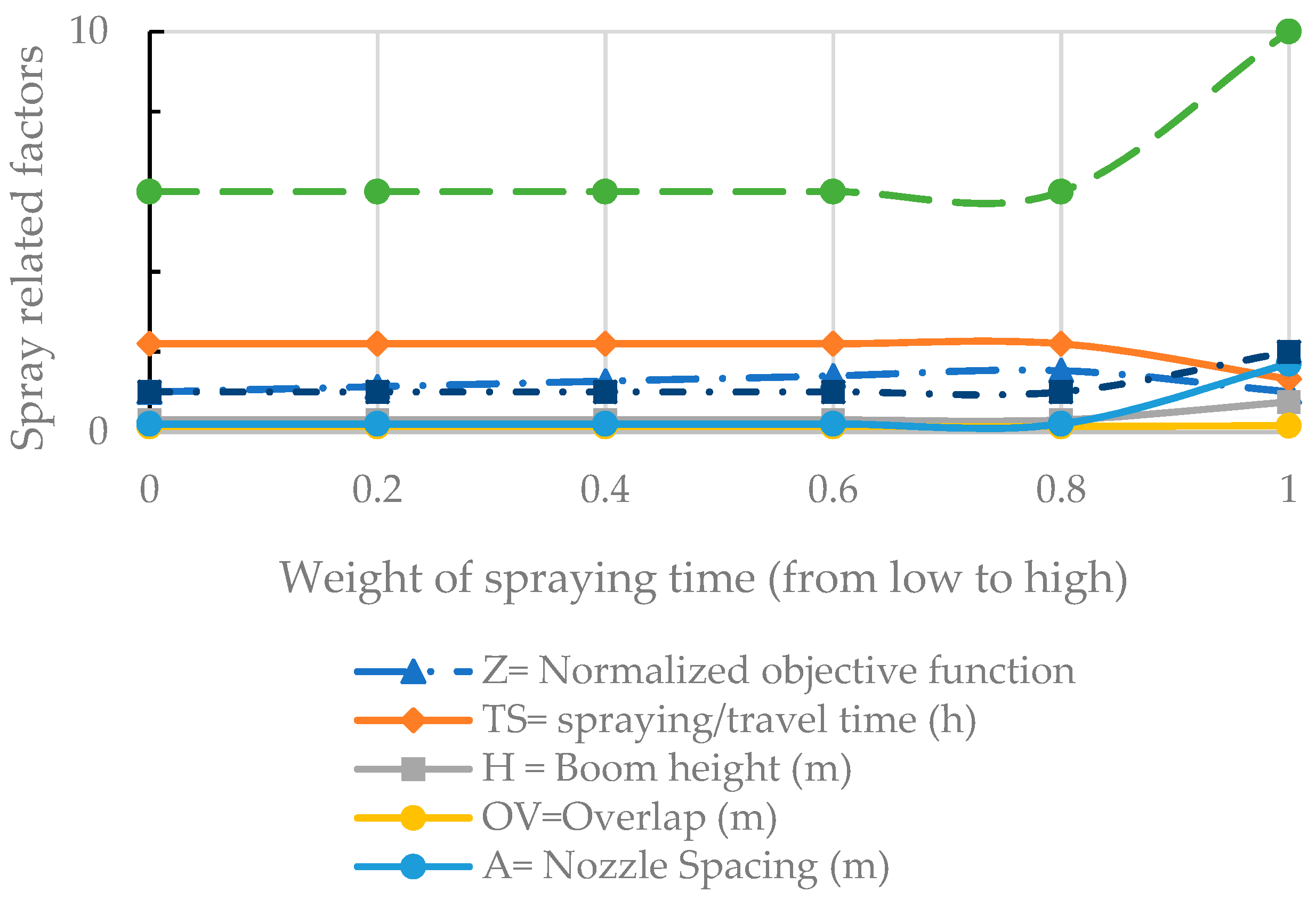
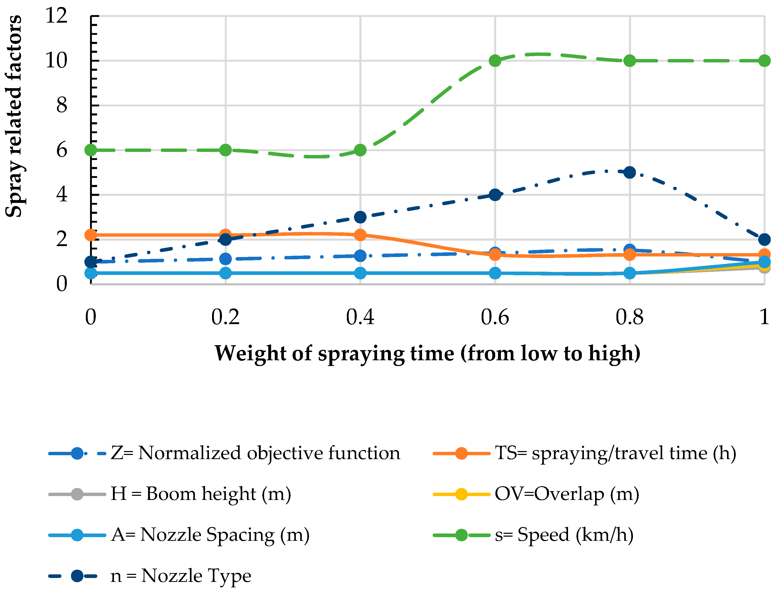
In this paper, a mathematical model was developed to select settings for spraying operations with the dual goal of jointly minimizing spraying time and drift proportions. The obtained bi-objective mixed integer nonlinear programming model was solved for a case study example published in the crop protection literature. Optimal solutions were obtained using the weighted sums method and the epsilon-constraint approach. The results showed that valid and reasonable solution can be obtained by selecting the appropriate combination of boom height, nozzle spacing, nozzle type, operating pressure, and tractor travel speed. The mathematical model developed in this study could be extended to include more factors such as evaporation, spray run-offs, and integrated into a mobile phone app to assist farmers in selecting the settings for their spraying operations.

The current mathematical model does not consider any specific crop and other drift factors such as evaporation and droplet sizes. Future research initiatives should target the integration of these factors. It would also be useful to conduct extensive field experiments with the goal of obtaining more granular data to feed into the bi-objective model to test its behavior on larger datasets. Furthermore, recent developments in the field of numerical simulation of drift losses can be leveraged to build joint simulation-optimization models to help farmers and decision makers in the selection of their spraying parameters.

References

1. Farm Bill. U.S. Congress. Food, Agriculture, Conservation, and Trade Act of 1990; Public Law 101–624: U.S. Farm Bill; The National Center for Agricultural Law Research and Information University of Arkansas, 28 November 1990; Available online: https://nationalaglawcenter.org/wp-content/uploads/assets/farmbills/1990-1.pdf (accessed on 23 November 2018).
2. Velten, S.; Leventon, J.; Jager, N.; Newig, J. What is sustainable agriculture? A systematic review. Sustainability 2015, 7, 7833–7865. [Google Scholar] [CrossRef]
3. Al-Heidary, M.; Douzals, J.P.; Sinfort, C.; Vallet, A. Influence of spray characteristics on potential spray drift of field crop sprayers: A literature review. Crop Prot. 2014, 63, 120–130. [Google Scholar] [CrossRef]
4. Pimentel, D. Environmental and economic costs of the application of pesticides primarily in the United States. Environ. Dev. Sustain. 2005, 7, 229–252. [Google Scholar] [CrossRef]
5. Oerke, E.C. Crop losses to pests. J. Agric. Sci. 2006, 144, 31–43. [Google Scholar] [CrossRef]
6. Huang, Y.; Zhan, W.; Fritz, B.K.; Thomson, S.J. Optimizing selection of controllable variables to minimize downwind drift from aerially applied sprays. Appl. Eng. Agric. ASABE 2011, 28, 307–314. [Google Scholar] [CrossRef]
7. Bahrouni, H.; Sinfort, C.; Hamza, E. Evaluation of pesticide losses during cereal crop spraying in Tunisian conditions. In Proceedings of the 10th International Congress on Mechanization and Energy in Agriculture, Antalya, Turkey, 14–17 October 2008. [Google Scholar]
8. Miller, P.C.H.; Butler, E.M.C. Effects of formulation on spray nozzle performance for applications from ground-based boom sprayers. Crop Prot. 2000, 19, 609–615. [Google Scholar] [CrossRef]
9. Nuyttens, D.; Baetens, K.; De Schampheleire, M.; Sonck, B. Effect of nozzle type, size and pressure on spray droplet characteristics. Biosyst. Eng. 2007, 97, 333–345. [Google Scholar] [CrossRef]
10. MacRae, R.J.; Hill, S.B.; Henning, J.; Mehuys, G.R. Agricultural Science and Sustainable Agriculture: A Review of the Existing Scientific Barriers to Sustainable Food Production and Potential Solutions. Biol. Agric. Hortic. 1989, 6, 173–219. [Google Scholar] [CrossRef]
11. Chao, F.; Chengsheng, Z.; Fanyu, K.; Jing, W. Effects of spray height and spray angle on spray deposition in tobacco plants. In Proceedings of the 6th IEEE Conference on Industrial Electronics and Applications, Beijing, China, 21–23 June 2011. [Google Scholar]
12. Teske, M.E.; Thistle, H.W. A simulation of release height and wind speed effects for drift minimization. Trans. ASAE 1999, 42, 583–591. [Google Scholar] [CrossRef]
13. De Jong, A.; Michielsen, J.M.G.P.; Stallinga, H.; Van de Zande, J.C. Effect of sprayer boom height on spray drift. In Proceedings of the 52nd International Symposium on Crop Protection, Gent, Belgium, 9 May 2000. [Google Scholar]
14. Iqbal, M.; Ahmad, M.; Younis, M. Effect of Reynold’s number on droplet size of hollow cone nozzle of environment friendly university boom sprayer. Pak. J. Agric. Sci. 2005, 42, 106–111. [Google Scholar]
15. Taylor, W.A.; Andersen, P.G.; Cooper, S. The use of air assistance in a field crop sprayer to reduce drift and modify drop trajectories. In Proceedings of the British Crop Protection Conference on Weeds, Alton, UK, 20–23 November 1989. [Google Scholar]
16. Miller, P.C.H.; Smith, R.W. The Effects of Forward Speed on the Drift from Boom Sprayers; British Crop Protection Council: Alton, UK, 1997. [Google Scholar]
17. Ghosh, S.; Hunt, J.C.R. Spray jets in a cross-flow. J. Fluid Mech. 1998, 365, 109–136. [Google Scholar] [CrossRef]
18. Heijne, B.; Wenneker, M.; Van De Zande, J.C. Air inclusion nozzles don’t reduce pollution of surface water during orchard spraying in the Netherlands. Asp. Appl. Biol. Intl. Adv. Pest. Appl. 2002, 66, 193–199. [Google Scholar]
19. Tobi, I.; Saglam, R.; Kup, F.; Sahin, H.; Bozdogan, A.M.; Piskin, B. Determination of accuracy level of agricultural spraying application in Sanliurfa/Turkey. Afr. J. Agri. Res. 2011, 6, 6064–6072. [Google Scholar]
20. Nuyttens, D.; De Schampheleire, M.; Baetens, K.; Sonck, B. The influence of operator-controlled variables on spray drift from field crop sprayers. Trans. ASABE 2007, 50, 1129–1140. [Google Scholar] [CrossRef]
21. Hwang, C.L.; Masud, A.S.M. Multiple Objective Decision Making—Methods and Applications, 1st ed.; Springer: Heidelberg/Berlin, Germany, 1979; pp. 21–283. [Google Scholar]
22. Ghayebloo, S.; Tarokha, M.J.; Venkatadri, U.; Diallo, C. Developing a bi-objective model of the closed-loop supply chain network with green supplier selection and disassembly of products: The impact of parts reliability and product greenness on the recovery network. J. Manuf. Syst. 2015, 36, 76–86. [Google Scholar] [CrossRef]
23. Lin, Y.; Linus, S. The global solver in the LINDO API. Optim. Methods Softw. 2009, 24, 657–668. [Google Scholar] [CrossRef]
24. Nadeem, M.; Chang, Y.K.; Venkatadri, U.; Diallo, C.; Havard, P.; Nguyen-Quang, T. Water quantification from sprayer nozzle by using particle image velocimetry (PIV) versus imaging processing technique. Pak. J. Agric. Sci. 2018, 55, 203–210. [Google Scholar]
25. Alaa, S.; Marek, M.; Stanisław, P.; Józef, S. Testing the uniformity of spray distribution under different application parameters. In Proceedings of the IX International Scientific Symposium Farm Machinery and Processes Management in Sustainable Agriculture, Lublin, Poland, 22–24 November 2017; pp. 259–264. [Google Scholar]
26. Nasir, S.H.; Nor, A.C.S.; Sidikand, J.M.S. Effect of nozzle type, angle and pressure on spray volumetric distribution of broadcasting and banding application. J. Mech. Eng. Res. 2013, 5, 76–81. [Google Scholar] [Green Version]
Figure 1. Drift-causing factors and spraying-speed parameters under consideration.
Agriengineering 01 00031 g001
Figure 2. Field layout and driving directions of tractor during spraying operation (example with four passes and three half rotations).
Agriengineering 01 00031 g002
Figure 3. Swath width (a) and spray sheet overlap between consecutive nozzles (b).
Agriengineering 01 00031 g003
Figure 4. Sensitivity analysis on the weights of objective function.
Agriengineering 01 00031 g004
Figure 5. Weighted sum results of 0 m minimum overlap.
Agriengineering 01 00031 g005
Figure 6. Weighted sum results of 0.1 m minimum overlap.
Agriengineering 01 00031 g006
Figure 7. Weighted sum results of 0.4 m minimum overlap.
Agriengineering 01 00031 g007