Novel Route Planning System for Machinery Selection. Case: Slurry Application

Abstract

The problem of finding an optimal solution for the slurry application process is casted as a capacitated vehicle routing problem (CVRP) in which by considering the vehicle’s capacity, it is required to visit all the tracks only once to fully cover the field, as well as complying with a specified targeted application rate. A key objective in this study was to determine an optimized coverage plan in order to minimize the driving distance in the field, while at the same time allowing for varying the application rate. The coverage plan includes the optimal sequence of tracks with a specified application rate for each track. Two algorithms were developed for optimization and simulation of the slurry application cast as capacitated operations. In order to validate the proposed algorithms, a slurry application operation was recorded, and the results of the optimization algorithm were compared with the conventional non-optimized method. The comparison showed that applying the proposed new method reduces the non-working distance by 18.6% and the non-working time by 28.1%.

1. Introduction

Capacitated field operations are operations that either involve input material flow such as fertilizing, or output material flow such as harvesting. Manure distribution operation requires considerable labor inputs and high-capacity specialized machines and equipment [1]. Furthermore, the odor and nuisance concerns related to the transportation and application of manure as well as the field traffic and soil compaction related to the spreading manure by heavy tankers especially in wet seasons, which impairs crop growth, are among the concerns which require farmers to optimize these operations to reduce the operational time and transportation costs [2,3].

As a solution, coverage planning methods can be used to increase the operational efficiency of the agricultural field operations [4,5,6], cutting the operational costs by improving the path tracking performance of the vehicle and by minimizing the overlapped area in the field [6]. Moreover, vehicle route planning (VRP) can be applied as a tool to reduce the operational time and costs by minimizing the total traveled distance in the field. In agriculture, VRP also has received increased attention and several studies show the application of VRP for planning the in-field operations [7,8,9]. Bochtis et al. (2013) [10] proposed an algorithmic method towards minimizing the total non-working distance traveled by an agricultural machine in the field. This involved expressing the field coverage as the traversal of a weighted graph and showed that the problem of finding an optimal traversal sequence is equivalent to finding the shortest path in the graph. By deploying algorithmically computed optimal sequences, the total non-working distance could be reduced by up to 50%, depending on the operating width and turning radius of the machine, shape of the fields and the type of conventional patterns that compared with the B-patterns. Moreover, it was shown that by exploiting the optimal headland patterns, apart from the reduction of non-working distance (followed by the reduction of the fuel consumption and the non-productive time), a reduction of soil compaction in the headland area will also be achieved [7].

Although the VRP has received considerable attention among computer scientists, operations management specialists, and others researching logistics, solving the problem by an exact algorithm is time demanding and computationally intractable [11]. Therefore, this challenge has led to the need to develop algorithms that can produce near-optimal solutions in a reasonable amount of time [12]. During the years, different solution approaches have been developed including exact algorithms (such as branch-and-bound [13,14] and branch-and-cut [15]), heuristic algorithms (such as the Clarke–Wright savings algorithm [16]), and metaheuristic algorithms (such as simulated annealing [17,18], genetic algorithms [19], tabu search [20], and ant algorithms [21]. Earlier, conventional heuristic algorithms were designed as a response to limited computer processing power. However, in recent years, meta-heuristic algorithms, such as simulated annealing, genetic algorithms, and tabu search, have been developed to perform a more thorough search of solution space. These algorithms are more computationally expensive where the time needed for calculations and the degree of optimality depend on the specifications of the problem and the design of the meta-heuristics.

Some coverage planning methods have been presented in the scientific literature [22,23,24]. However, the case of capacitated operations has not been covered extensively. Ali et al. (2009) [25] proposed a practical planning approach for harvesting a field with several capacitated combine harvesters and tractor-trailers. Jensen et al. (2015) [26] presented an algorithmic method for the optimization of capacitated field operations using the case of liquid fertilizing. The presented method in this study avoids turnings within the main cropping area of the field and limits all the maneuvers to the headland part. As a result, there is less soil compaction in the inner part of the field in comparison with the previously mentioned approaches.

The objective of this paper is to develop an approach for the optimization of capacitated field operations such as manure application in the field. The target users are farmers and agricultural advisers who are interested in reducing the operational cost and the environmental impacts whilst maximizing the field efficiency. The specific objectives included:

• Decompose the fertilizing operation, by considering the operations elements (such as performing the main task) and unproductive elements (such as turnings in the headland part and idle transportation), to determine the operational performance of the machinery. Farmers’ current practices are used for validating and benchmarking the proposed algorithm and model.
• Develop an algorithm and tool to solve this specific field coverage problem with optimized application rates and minimized driving distances for all individual tracks in the field.
• Develop an approach and tool to help farm managers to select the proper tank volume for the machinery system given specific constraints.

2. Materials and Methods

2.1. Characteristics of the Slurry Application

In capacitated operations such as slurry application, the depot will be visited several times for refilling to complete the task. The number of tracks covered in each tour (a path that starts and ends at the depot) depends on the capacity of the slurry tank and the application demand of those tracks. The demand of each work-area can be calculated by multiplying the targeted application rate (L/m²) to the total area of that track (m²). The target application rate is the dosage of applied manure which is predetermined to meet crop nutrient requirements. In the manure distribution process, farmers prefer to go to the field with a full tank and return to the depot with the empty tank. Therefore, the summation of applied material in the visited tracks for each tour should be equal to the volume of the slurry tank. Thus, by adjusting the demands of a group of tracks, it is possible to cover them by one load. In this study and based on the agronomical and environmental standards [27], a target application rate was considered for the field and an arbitrary tolerance of ± 30% was considered for adjusting the tracks’ demand according to the information derived from a survey from farmers.

2.2. Mathematical Formulation

As mentioned before, the field route planning can be cast as a VRP problem which consists of determining a set of routes with minimum traveled distance for a vehicle, starting and ending at a single depot and satisfying the demand of the tracks with the constraints that each track is covered exactly once, and the total demands of the tracks in each route do not exceed the capacity of the vehicle. Bochtis D and Vougioukas S [7], formulated this problem as a weighted graph $G=\left(V, E\right)$, where $V=N\mathrm{U}\left\{0\right\}$, is the set of all vertices and $N=\left\{1, 2, 3\dots n\right\}$ is the set of nodes and $E$ is the set of all edges in the graph. The depot is represented by vertex $0$ and the nodes in set $N$ are denoted as the customers. For each edge $e_{ij}\in E ,i\ne j$, a non-negative cost $C_{ij}$ is considered as transit cost. Each node $i\in N$ is associated with a non-negative demand $d_i$.

The objectives or criteria considered in this study are: (I) each node is visited exactly once, (II) all routes start and end at the depot, (III) for each route, the total demand should be equal to the vehicle capacity VC in order to satisfy the criteria of returning to the depot with an empty tank, (IV) the application rate for each track should fit in the defined range (± 30% target application rate), (V) minimizing the non-working distance traveled by the vehicle.

All the applied variables and parameters in the following formulas were defined in

Table 1. Definition of the symbols that presented in the mathematical formulation of the problem.

Symbol	Definition
$X_{ij}$	Decision variable
$C_{ij}$	Non-negative transit cost
$d_{ij}$	Corresponding demand for edge $e_{ij}$
$A{R}_{ij}$	Application rate for edge $e_{ij}$
$VC$	The vehicle capacity
$TAR$	Target application rate

.

$$\begin{gathered} X_{ij}=\{ \begin{array}{c}1:if the vehicle immediatly goes from vertice i to vertice j \\ 0 :if the vehicle need to visit depot for unloading process \end{array} \\ {d}_{ij}=the corresponding demand of edge e_{ij} \end{gathered}$$

(1)

The objective function can be defined as follows:

$$Min : {{\displaystyle \sum }}_{i\in V}{{\displaystyle \sum }}_{j\in V}{C}_{ij}{X}_{ij}$$

(2)

The constraints are as follows:

$${{\displaystyle \sum }}_{j\in V}{X}_{ij}=1 , \forall i\in V$$

(3)

$${{\displaystyle \sum }}_{i\in V}{X}_{ij}=1 , \forall j\in V$$

(4)

$${{\displaystyle \sum }}_{i,j\in V}{X}_{ij}A{R}_{ij}{d}_{ij}=VC , \forall \left(i,j\right)\in V$$

(5)

$${{\displaystyle \sum }}_{i\in V}{X}_{iK}-{{\displaystyle \sum }}_{j\in V}{X}_{kj}=0 , \forall k\in V$$

(6)

$$\left(1-30\%\right)TAR\le A{R}_{ij}\le \left(1+30\%\right)TAR , \forall \left(i,j\right)\in V$$

(7)

$$X_{ij}\in \left\{0,1\right\} , \forall \left(i,j\right)\in V$$

(8)

The Equations (3) and (4) state that only one of the sibling nodes appears in the solution. Equation (5) specifies that the total summation of demand related to each trip should be equal to the capacity of the vehicle in order to satisfy the criteria to return to the depot with an empty tank. Equation (6) represents that if the vehicle starts covering a track $K$, it will leave the track at the end of the process. Equation (7) ensures that the application rate for each edge will fall within the stipulated range. Lastly, Equation (8) states the type of decision variable $X_{ij}$.

2.3. Solution Representation

The proposed method denotes a novel precision agriculture method, that combines organic and artificial fertilizers application on agricultural fields while at the same time optimize the in-field transport and subsequent soil compaction. According to this new method, the complete process of fertilization of a field is executed in two steps. Firstly, a slurry tanker is used to distribute the liquid organic manure on the field by adjusting the agronomic required target application rate for each track and minimizing the non-working distance as determined by the proposed method. As a result, an organic fertilizer’s application map will be generated to be used in the next step. This next step comprises an artificial fertilizer spreader applying variable rate fertilizer based on the previously generated map to meet the full crop nutrient requirements and at the same time minimize the non-working distance. This novel method will minimize the overall combined in-field traffic and the non-working driving distances by performing all the optimal turnings and maneuvers in the headland area. Moreover, it will reduce the soil compaction in the main cropping area of the field by avoiding turnings in-field and empty transport in the main part of the field. This is achieved by adjusting the fertilizer’s application rate to let the machine’s operator cover the entire track to reach the headland part. According to the machine’s variable rate application capability, the planned actual application rate for each track is going to be determined as a stipulated deviation from the target rate for a field and crop.

2.3.1. Field Representation

The first step in the field area coverage planning process is to generate a geometrical representation of the selected field. One of the common methods in this concept is using the spatial configuration planning approach, which applies the geometric primitives to represent the field [10]. This method consists of three tasks: First, representing the field with simple geometry shapes; second, determining the driving direction in the field and; third, generating the work areas (tracks) based on the driving direction. The output from this method is a set of line segments or polylines which depicts the fieldwork areas and headland passes that can be followed by the machine.

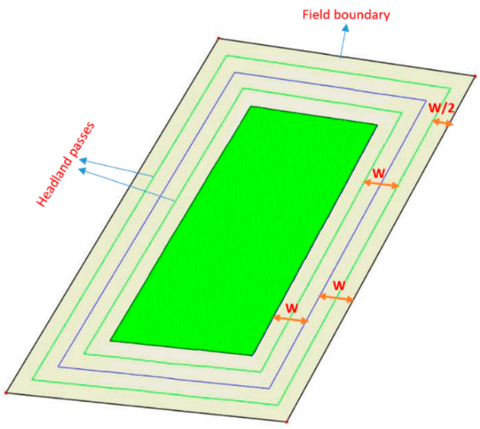
Headland Area Generation

The field headland area, as showed in Figure 1, is generated by inwardly offsetting the field’s boundary equal to the multiplication of the operating width of machine (W) times to the number of headlands passes (h). The distance from the field boundaries to the first headland pass is equal to W/2, while the distance between subsequent passes of headland equals to the W.

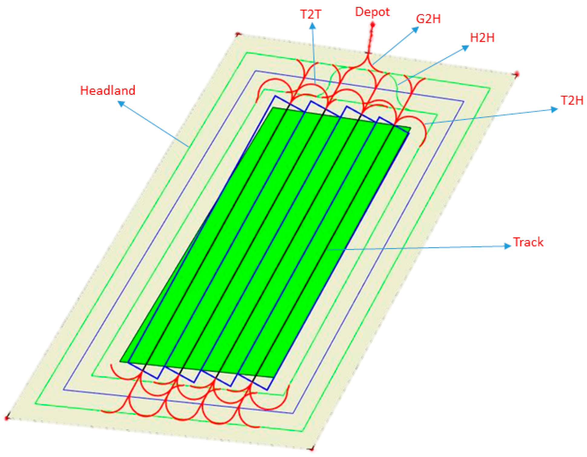
Track Generation and Edge Type

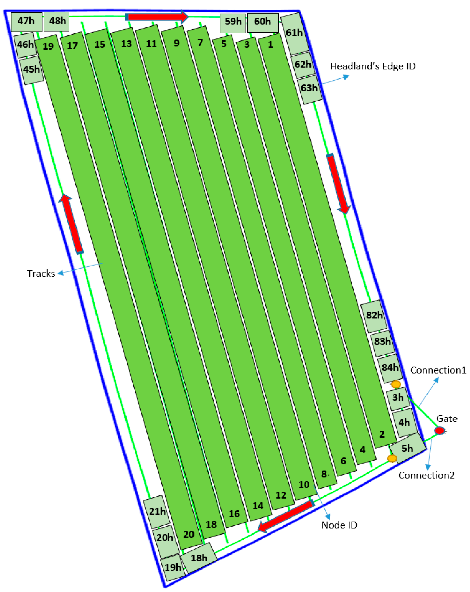
A set of straight tracks parallel to the defined driving direction is generated. Each track is represented by two ends (nodes) that are located on the inner field boundary. The distance between subsequent tracks is equal to (W). Figure 2 demonstrates the generated work rows with different types of edges in the field.

There are six types of edges between each pair of the vertices and each defined edge has a length:

• Gate to Headland (G2H): two edges connect the gate to the headland path
• Headland: the connection between two subsequent vertices in headland path
• Track: the connection between two pairs of nodes (two ends of a fieldwork area). Once a vehicle selects one end as the track entry, it has to finish the operation in the current track and exits at the opposite end of the current track before moving to another track.
• Track to Headland (T2H): the connection between track nodes and vertices in the headland path
• Track to track (T2T): the connection between the end nodes of two adjacent tracks
• Headland to headland (H2H): the connection between two headland paths

For the first type, the edge cost is the traveled distance between the headlands’ vertices and the field’s gate. For the second type, the edge cost is the length of the headland edge when the vehicle is operating in unproductive mode. For the third type, the edge cost is the length of the edge when the vehicle is operating in an unproductive mode. For the last type, the edge cost is the distance corresponding to the headland turning from the exit point of the current track to vertices in the headland path.

2.4. Optimization Algorithm

The problem explored in this study is to find the optimal traversal sequence of fieldwork tracks with an adapted application rate for each track to minimize the non-working driving distance in the field. Since there is a large discrete search space in this problem, it can be classified as a well-known VRP NP-hard problem where tracks’ nodes will be visited instead of customers and the vehicle will refill at the depot. The meta-heuristic algorithm simulated annealing (SA) is applied to find the global optimum solution for this problem. The optimization model was developed using the PYTHON programing language (version 3.7) [28]

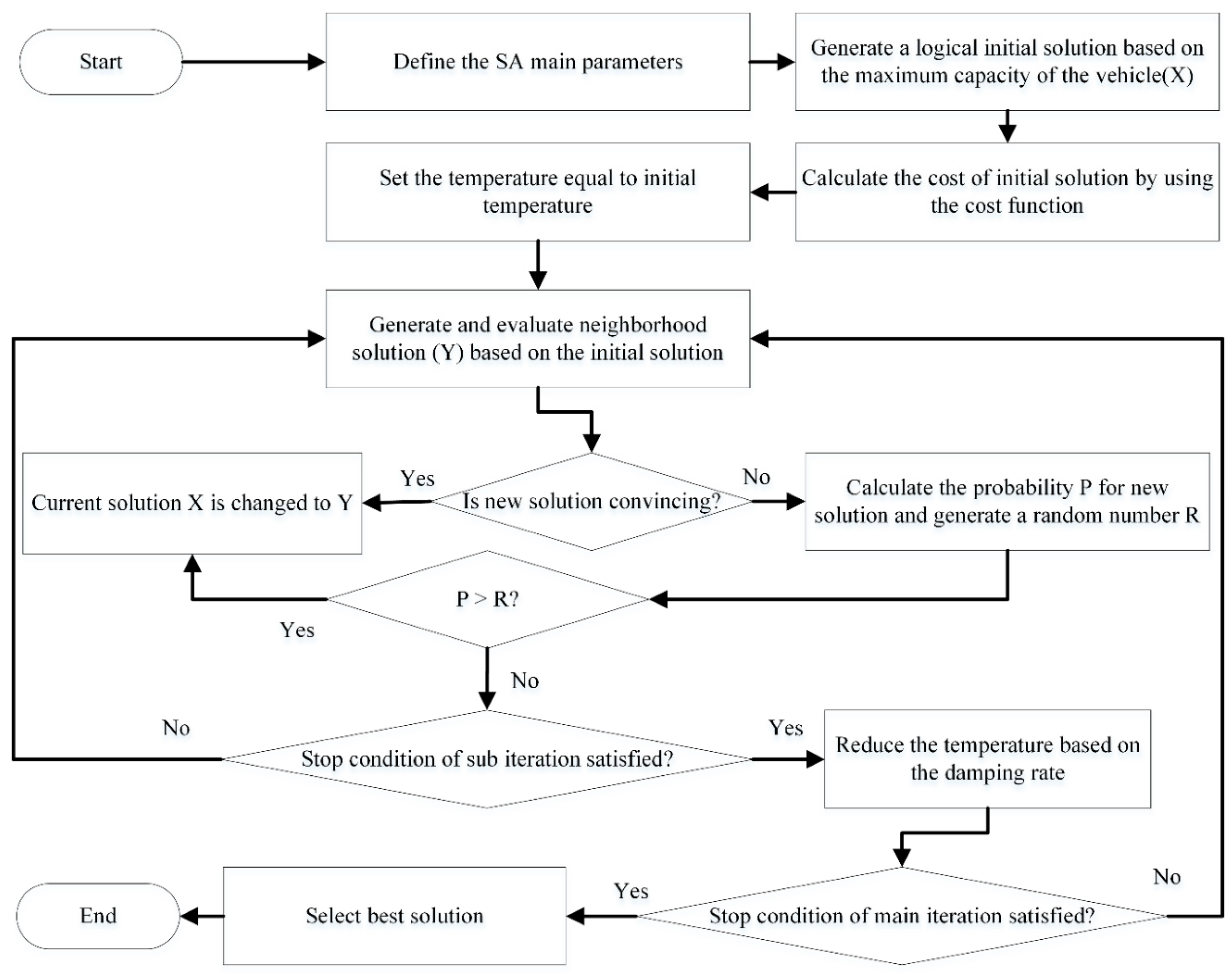
2.4.1. SA Algorithm

The simulated annealing as a stochastic algorithm is used in this study to investigate the near-optimal solution. This method implemented in several problems in various fields such as computer design, route planning, image processing, etc. The performance structure of this algorithm is based on the simulation of the cooling process, which called annealing where a solid is gradually cooled. The SA algorithm has some primary features such as the initial temperature, cooling rate, and termination policy, which should be defined carefully in advance since the performance of the algorithm depends on them.

Table 2. Primary features of the simulated annealing (SA) algorithm.

Main Iterations	Internal Iterations	Initial Temperature	Cooling Rate
2000	60	2000	0.9

represents the corresponding values for the primary features of the SA algorithm. For instance, at the beginning when we have a higher temperature, the probability of accepting newer worse solutions is high and by spending time, it will decrease. By this ability, the SA algorithm enabled to search of all solution space and escape from trapping in local minima [29].

The overview of the SA algorithm could be listed as the following Flowchart (Figure 3):

Neighborhood Operators

A new solution in the SA algorithm can be generated by applying various neighborhood operators on an initial solution. Random swaps, random swaps of subsequences, random insertions, random insertions of subsequences, reversing a subsequence, and random swaps of reversed subsequences are among the neighborhood operators, which is applied in this study. All mentioned operators demonstrated with an example in the following table (

Table 3. Applied neighborhood operators.

	Random swaps
B*	0	9	4	7	2	5	12	0	13	18	19	16	0
A*	0	9	4	7	2	5	12	0	18	13	19	16	0
	Random insertions
B	0	9	4	7	2	5	12	0	13	18	19	16	0
A	0	9	4	5	7	2	12	0	13	18	19	16	0
	Reversing a subsequence
B	0	9	4	7	2	5	12	0	13	18	19	16	0
A	0	9	12	5	2	7	4	0	13	18	19	16	0
	Random swaps of subsequences
B*	0	9	4	7	2	5	12	0	13	18	19	16	0
A*	0	5	12	2	9	4	7	0	13	18	19	16	0
	Random insertions of subsequences
B	0	9	4	7	2	5	12	0	13	18	19	16	0
A	0	9	2	5	12	4	7	0	13	18	19	16	0
	Random swaps of reversed subsequences
B	0	9	4	7	2	5	12	0	13	18	19	16	0
A	0	12	5	2	7	4	9	0	13	18	19	16	0

* B = Before, A = After. Numbers with bold changed after applying the neighborhood operator.

).

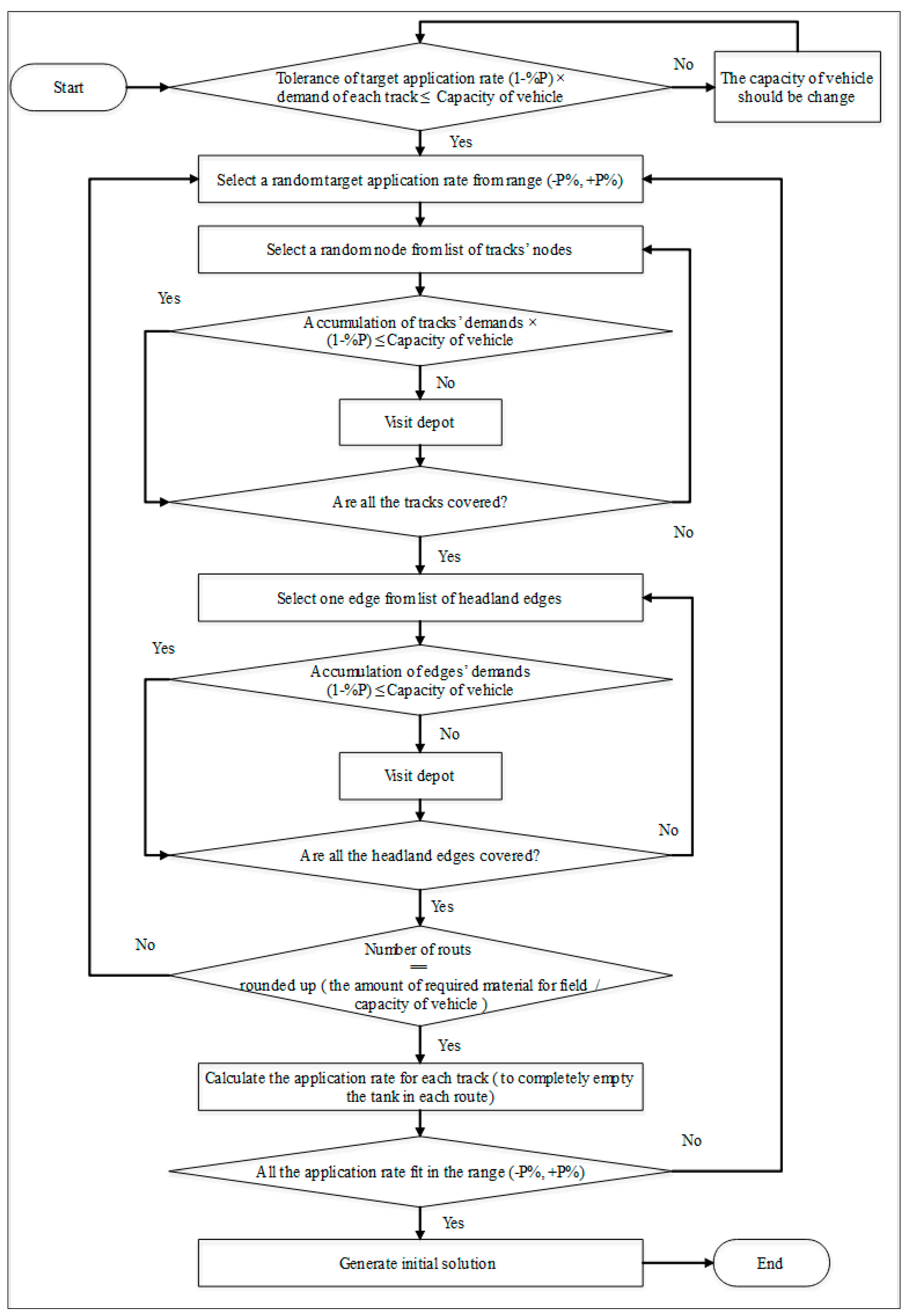
Initial Solution

In the fertilization process to avoid crossing the already applied area, first the inner part of the field and later the headland parts are going to be covered. The following flowchart (Figure 4) represents an overview of the process of generating an initial solution.

2.4.2. Application Rates

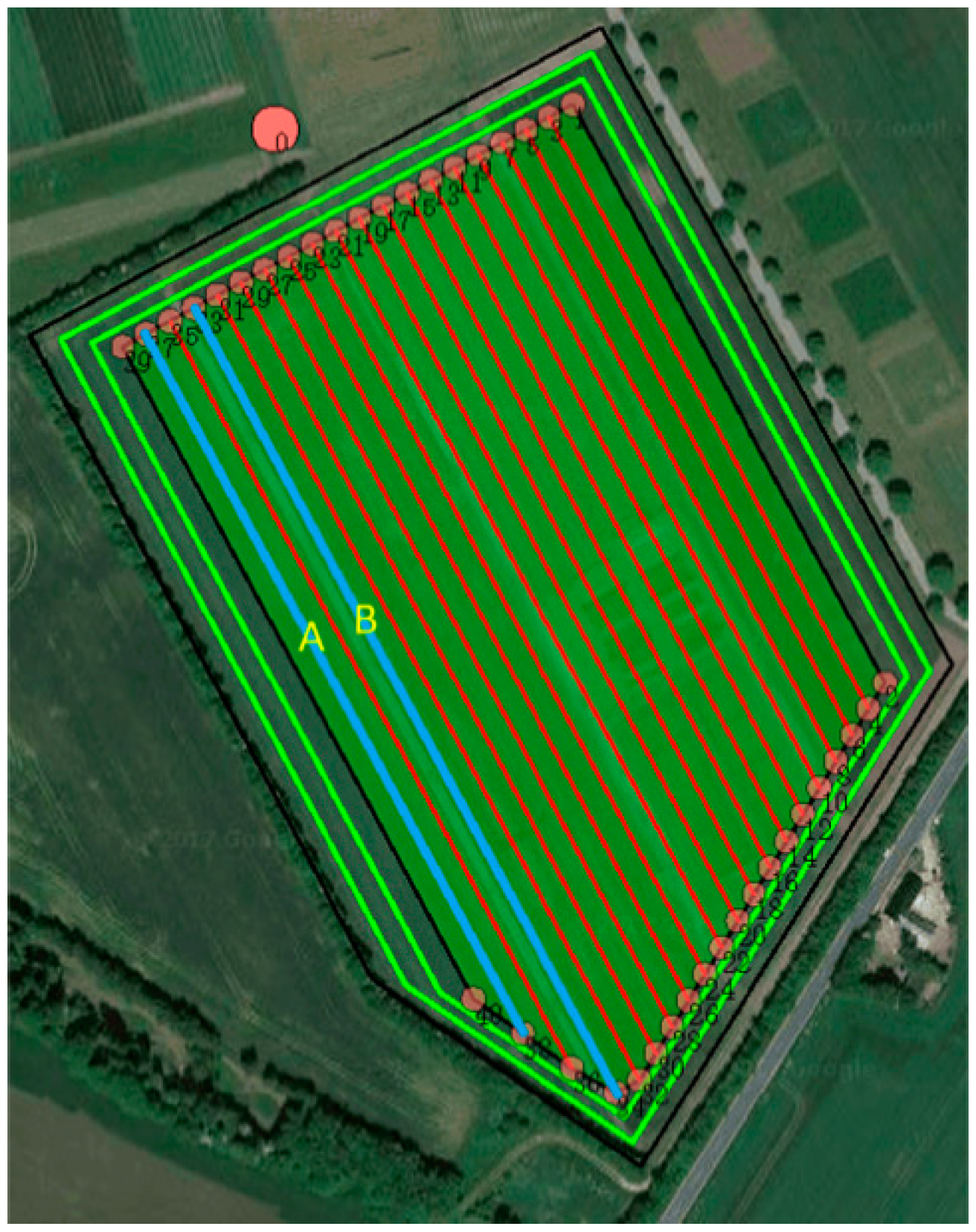
In order to show the process of calculating the application rate for the tracks, a sample route with two tracks ([0, A, B, 0]) were selected and demonstrated in Figure 5. The required data for calculating the application rate for the tracks in one load are the length of tracks, the demands, the capacity of the slurry tank, the working width of the machine, and the deviation tolerance of the stipulated target application rate. All the applied variables and parameters in the process of calculating the application rates are defined in

Table 4. Definition of the symbols used in the calculation of the application rates.

Symbol	Definition
$TDMax$	The total demand of all the tracks in one route with a maximum extension
$VC$	Vehicle capacity
$W$	Working width of the machine
$d_i$	The demand for the track $i$
$L_i$	Length of the track $i$
$P$	Percentage (between 0-30)
$R$	The remaining amount of material inside the tank
$D$	Distribution of $R$ through the route
$m_i$	The amount that should be added to the track $i$
$A{d}_i$	Adjusted demand for the track $i$
$A{R}_i$	Application rate for the track $i$

.

$$TDMax={{\displaystyle \sum }}_i{d}_i\ast \left(1-\%P\right);\forall \mathrm{i}\in \left\{A,B\right\}$$

(9)

$$R=VC-TDMax$$

(10)

$$D=R/{{\displaystyle \sum }}_i{L}_i;\forall \mathrm{i}\in \left\{A,B\right\}$$

(11)

$$m_i=D\ast L_i ; \forall i\in \left\{A,B\right\}$$

(12)

$$A{d}_i=d_i\ast \left(1-\%P\right)+m_i ; \forall i\in \left\{A,B\right\}$$

(13)

$$A{R}_i=A{d}_i/\left(L_i\ast W\right) ; \forall i\in \left\{A,B\right\}$$

(14)

2.4.3. Cost Matrix Generation

The cost matrix represents the transition cost between every pair of vertices of the field graph. Let $M$ be the $n\ast n$, $n=\left|V\right|$ matrix with element $C_{ij}$, where $C_{ij}$ is the transition cost from vertex $i$ to $j$ when $i\ne j$ and is equal to 0 when $i=j$. In order to calculate the $C_{ij}$, the generated field representation in the previous section is transformed as an undirected graph $G=\left(N,E\right)$, where $N=\left\{n_0,n_1,\dots ,n_n\right\},n\in Z$ is the set of nodes consisting of all ending points of headland passes, fieldwork tracks, and connection paths, where $E=\left\{\left\{n_i,n_j\right\},\dots \right\},n_i,n_j\in N$ is the set of edges representing all headland passes, fieldwork tracks, and connection paths. Each edge $\left\{n_i,n_j\right\},i\ne j$ is associated with a weight, which corresponds to the actual length from node $n_i$ to node $n_j$. Based on the derived graph, the distance between every pair of vertices can be computed by using the shortest path search algorithm (Dijkstra algorithm). It needs to be clarified that the vertex set $V$ is a subset of $N$, since $V$ only consists of depots and ending points of all tracks, while $N$ is the set of all points. In the cost matrix, only the distance between every pair of vertices in $V$ is stored as every $C_{ij}$ element.

2.5. Simulation Algorithm

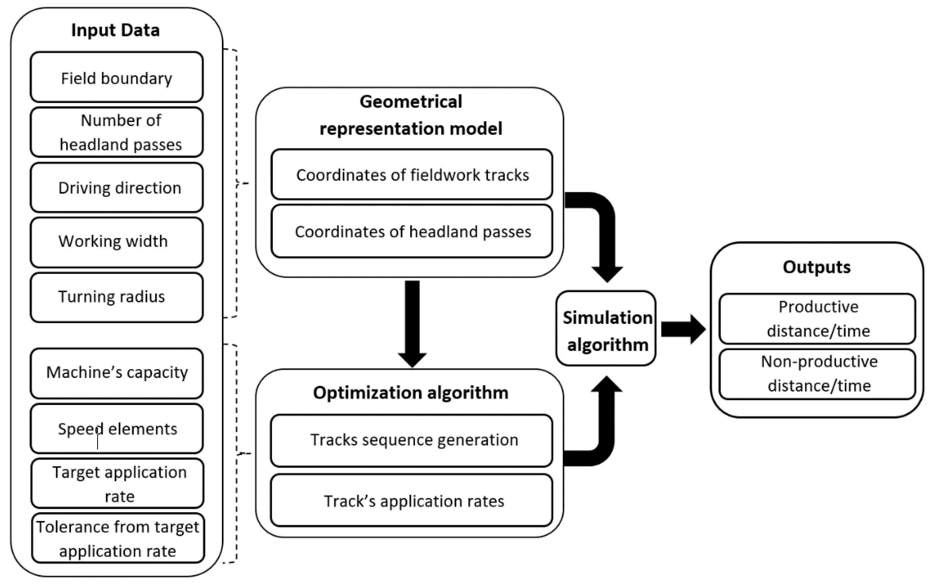
A simulation model for the slurry application system is developed to calculate the total estimated non-working traveled distance (includes turnings’ length and reloading distance) and the total estimated non-working time (includes turnings’ time and reloading time). The refill event happens at the depot when the slurry tank is emptied. Hence, the simulation model calculates the transport distance and time and reloading time. An overview of the model is presented in Figure 6. The simulation model was developed using the MATLAB^® technical programming language (version R2018b) [30]. In the simulation model, a tool is developed to geometrically represent the field. The boundary of the field and headland areas demonstrated by the polygons and the inner part of the field is partitioned as a series of parallel working-areas (tracks). The input data for the geometrical representation model are the field boundary, number of headlands passes, driving direction, working width, and turning radius of the applied machine. The optimal sequence of tracks and their proper application rates determined by the optimization algorithm. The input data for the optimization algorithm consist of coordinates of fieldwork tracks, coordinates of headland’s passes, the capacity of the slurry machine, machine’s traveling, working and turning speed, the target application rate for the field, and the acceptable tolerance from the target application rate. The output of the geometrical representation model and the optimization algorithm was used as an input for the simulation algorithm. The output of the simulation algorithm is the segmentation of the task time and traveled distance for each part of the operation (productive or non-productive).

3. Results

In order to validate the proposed algorithm and evaluate the enhancement in the operation efficiency caused by the optimized plan as compared to the operation executed based on conventional planning, a shallow injection fertilizing operation was performed and recorded. As a case study, a sample field was considered for comparison between the conventional and optimized plans. The conventional method indicates that farmers prefer to fill the slurry tank at the depot and after visiting the field, the distributor is returned to the depot with an empty tank. It means that all the capacity of the slurry tank should be applied in the field before returning to the depot. When adhering to this method, sometimes it is not possible to find a combination of tracks where the total required material for covering them is exactly equal to one load of the applicator. The ramifications of this are that farmers perform turns in the main part of the field or emptied the rest of the material into another field.

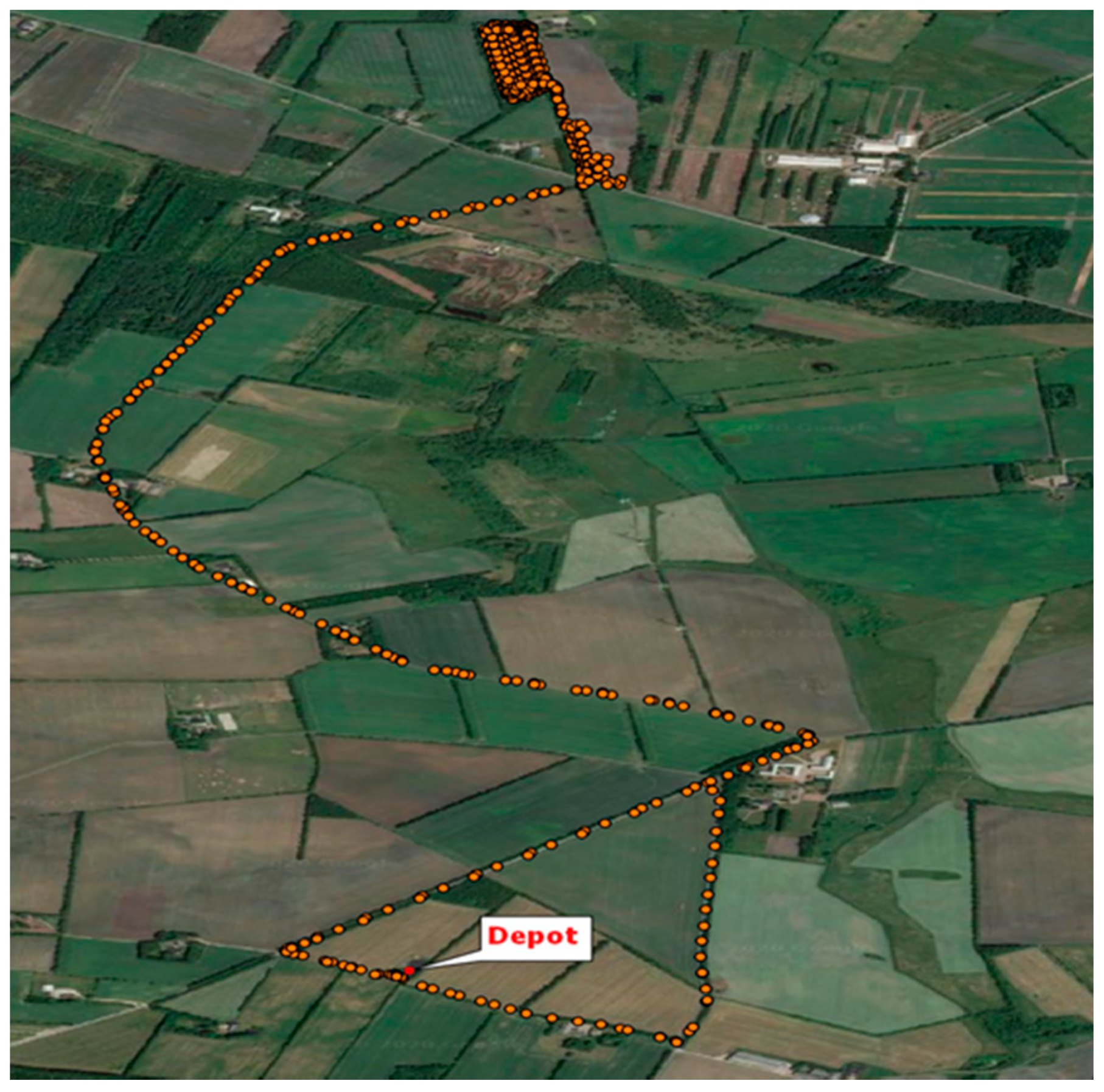
Figure 7 demonstrates the target field and the location of slurry storage (Depot). The yellow points show the log file for the slurry application in that field. All the information regarding the field and characteristics of the applied machine presented in

Table 5. Input data for the optimization and simulation models.

Field’s location Depot’s location Working width (m)	Latitude: 55°34’50.63” N, Longitude: 8°59’3.76” E Latitude: 55°34’47.4366” N, Longitude:8°59’07.0432” E 7
Turning radius (m)	12
Capacity (L)	33,000
Working speed (m/s)	1.6
Non-Working speed (m/s)	3.82
Target application rate (L/m2)	4
Tolerance from target application rate (%) Number of headlands passes	30 1

. Moreover, the information corresponding to the properties of the generated tracks showed in

Table 6. Tracks’ properties.

Track ID	1	2	3	4	5	6	7	8	9	10
Nodes	(1,2)	(3,4)	(5,6)	(7,8)	(9,10)	(11,12)	(13,14)	(15,16)	(17,18)	(19,20)
Demands (L)	7888	8155	8390	8613	8838	9061	9277	9485	9693	9694
Length (m)	227.2	234.9	241.7	248.1	254.6	261	267.2	273.2	279.2	279.2

. These data are going to be used later in the optimization and simulation algorithm to calculate the optimal coverage plan.

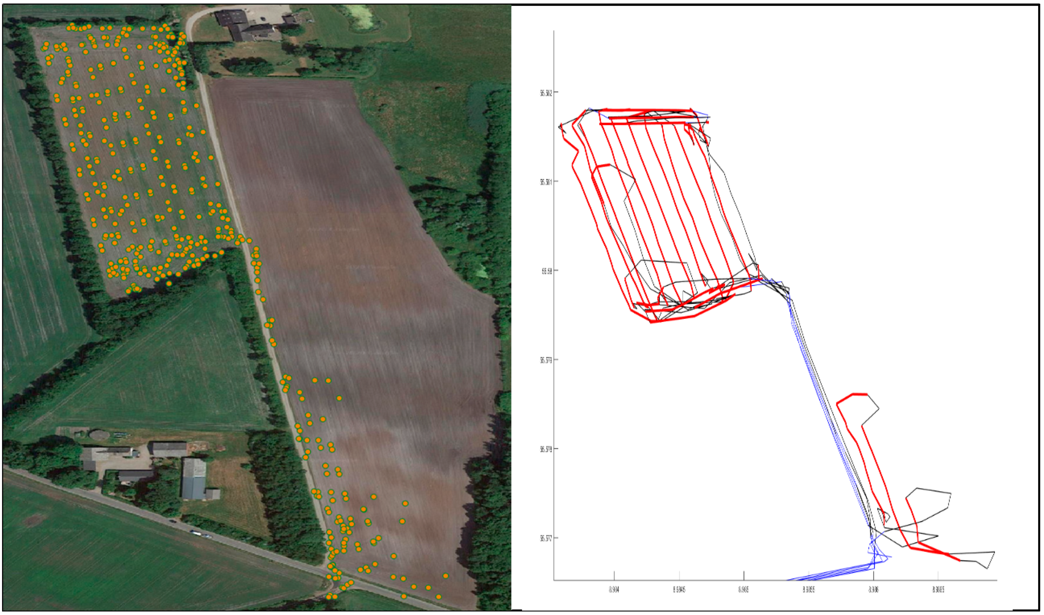
Figure 8 demonstrates how the farmer executed the slurry application on the target field. In terms of the conventional method, the order of covering tracks are as follows: [0,19,12,15,18_1,0], [0,14,5,10,18_2,a,0], [0,1,8,3,b,c,0]. In each path, the slurry tank starts from the depot (zero represents the depot) with full capacity (33,000 L) and it covers some tracks and when the tank is empty it returns to the depot for reloading. In the first path, tracks numbers 10, 6, 8, and part of track 9 were covered. In the second tour, the tracks’ ID 7, 3, 5 and the rest of the track ID 9 were covered and the total required material for these tracks is 31,437 (liters) and there is 1563 (liters) of slurry remained in the tanker and the farmer decided to empty the tank into another field besides the target field (part a). The last route starts from the depot and it includes the tracks ID number 1, 4, 2, and remained material (8344 L) emptied in the adjacent field (parts b and c).

A log file was generated using recorded GPS data of the slurry distributor by considering a constant application rate for all the tracks. The information in the log file was used for calculation of non-working time and distance for a slurry tank in the field. The non-working time is the accumulation of GPS time when the distributer does not apply fertilizer in the field or when it is out of the field. The non-working traveled distance can be determined by calculation of the number of meters traveled by the machine in the non-working time.

Table 7. The results of the conventional method.

Conventional Method
Non-Working Time (minutes)	Non-Working Distance (meter)	Working Time (minutes)	Working Distance (meter)
87.87	26,400	25.77	3406

demonstrates the results of the analysis for the conventional method.

Based on the input data mentioned in Table 5 and Table 6, the geometrical representation model divided the target field into 10 working areas with one headland part. Figure 9 demonstrates the target field with all the characteristics such as field boundaries, tracks, headland area, and the gate of the field. By applying the proposed method in this study, an optimal solution was generated for this field.

Table 8. The optimized solution with the simulation results.

Optimized Solution	<0, 12, 13, 16, 17, 0, 20, 9, 8, 5, 0, 4, 1, 3 h, 4 h, 5 h, 6 h, 7 h, 8 h, 9 h, 10 h, 11 h, 12 h, 13 h, 14 h, 15 h, 16 h, 17 h, 18 h, 19 h, 20 h, 21 h, 22 h, 23 h, 24 h, 25 h, 26 h, 27 h, 28 h, 29 h, 30 h, 31 h, 32 h, 33 h, 34 h, 35 h, 36 h, 37 h, 38 h, 39 h, 40 h, 41 h, 42 h, 43 h, 44 h, 45 h, 46 h, 47 h, 48 h, 49 h, 50 h, 51 h, 52 h, 53 h, 54 h, 55 h, 56 h, 57 h, 58 h, 59 h, 60 h, 61 h, 62 h, 63 h, 64 h, 65 h, 66 h, 67 h, 68 h, 69 h, 70 h, 71 h, 72 h, 73 h, 74 h, 75 h, 76 h, 77 h, 78 h, 79 h, 80 h, 81 h, 82 h, 83 h, 84 h, 0>
Non-Working Time (minutes)		Non-Working Distance (meter)	Working Time (minutes)	Working Distance (meter)
63.15		21489	22.25	3248

shows the results of the optimization and simulation model for the optimal solution. The solution is an optimal coverage plan which first covers the inner part of the field and then the headland area. The numbers without a letter (h) in the solution represent one of the track’s sibling nodes. Moreover, headland passes divided into some edges which they are distinguished by letter (h). Zero represents the depot and in the solution, when there is a zero, it means a reloading event happened.

To have a better comparison between the optimal solution and the conventional one, the time and distance from the field’s gate to the depot was calculated and added to the optimal solution (traveled distance from the gate to the depot and back to the gate = 6861 m; time to go from gate to the depot and back to the gate = 1184 s). Since in the optimal solution there are three loads, therefore, the time and distance from the gate to the depot should be multiplied by 3 and added to the non-working time and distance of the optimal solution.

The comparison showed that applying this new method can reduce the non-working driving distance by 18.6% and the non-working time by 28.1%. In the first tour of the conventional method, tracks’ ID (10, 6, 8) are covered completely and due to the limited capacity, part of the track 9 is covered in that tour and machine-turned through the cropping part of the field to go back to the depot for refilling. These maneuvers inside the agricultural main field have negative effects on the soil and can reduce the crop’s yield [7]. However, the proposed method in this study avoids turnings through the main field by adjusting the application rates to an optimal value to let the machine operate the entire track.

Table A1. List of application rates for case study field-capacity 33 m^3.

Node/Edge ID	Application Rate (L/m2)	Node/Edge ID	Application Rate (L/m2)
1	3.114799011967676	48 h	3.114774926773009
4	3.1147990119676754	47 h	3.114774926773009
5	4.6061000129481195	46 h	3.1147806166643486
8	4.6061000129481195	45 h	3.1147736783248767
9	4.60610001294812	44 h	3.114774926773009
12	4.36275440399874	43 h	3.114774926773009
13	4.36275440399874	42 h	3.1147762950571463
16	4.36275440399874	41 h	3.114800113322044
17	4.36275440399874	40 h	3.114774926773009
20	4.60610001294812	39 h	3.114774926773009
84 h	3.114833305549154	38 h	3.1147938549403227
83 h	3.114774926773009	37 h	3.1148003337060293
82 h	3.114774926773009	36 h	3.114774926773009
81 h	3.1148054910798435	35 h	3.114774926773009
80 h	3.114782546605226	34 h	3.1147341965638637
79 h	3.114793927303264	33 h	3.1148008560895373
78 h	3.114801606808676	32 h	3.114774926773009
77 h	3.114779348093042	31 h	3.114821230419206
76 h	3.1148156792952406	30 h	3.114896876687335
75 h	3.1147597405964764	29 h	3.1148156792952406
74 h	3.1147849713320523	28 h	3.114802898522297
73 h	3.114774926773009	27 h	3.1147901062639725
72 h	3.114781948008852	26 h	3.114774926773009
71 h	3.114763778934655	25 h	3.1148240581428697
70 h	3.114774926773009	24 h	3.1147950430878066
69 h	3.114740814750495	23 h	3.1148096816331345
68 h	3.114821963757087	22 h	3.1147722039444474
67 h	3.114812326616211	21 h	3.1147917310714286
66 h	3.1147999933614714	20 h	3.114803983493116
65 h	3.1148040212860635	19 h	3.1147879046797193
64 h	3.1148080403016585	18 h	3.1147997877656945
63 h	3.1147985147811466	17 h	3.114812020602183
62 h	3.1147991732911824	16 h	3.114800423314475
61 h	3.114795397917765	15 h	3.114815641025888
60 h	3.1148079782211164	14 h	3.1148101314088783
59 h	3.1147993692355422	13 h	3.114817787296218
58 h	3.1148014774813753	12 h	3.11480164195349
57 h	3.114786930335023	11 h	3.114785606390021
56 h	3.1148056420388746	10 h	3.1148133771671582
55 h	3.1147944605105216	9 h	3.1148151959511368
54 h	3.114808623307024	8 h	3.114785915868141
53 h	3.114810686533339	7 h	3.11478570426507
52 h	3.114793847126731	6 h	3.1148212190007927
51 h	3.1148053372155053	5 h	3.1147885124251764
50 h	3.1147978635235076	4 h	3.1148045618969324
49 h	3.114732898915732	3 h	3.114806305217886

in the Appendix A part, demonstrates the values of application rates for the generated optimized solution. In the second tour of the conventional method, to empty the slurry tanker, the farmer covered a small part of the adjacent field. The amount of applied slurry in the part (a) is equal to 1563 L and the machine traveled 329 m to reach the (a) part. Moreover, in the same situation, the vehicle traveled 342 m to arrive at the parts (b and c). The amount of slurry applied in these parts is equal to 8344 L. However, the proposed method in this study avoids these travels by adjusting the application rates to certain values that the machine’s capacity fully used and at the end of each tour there is no remaining slurry in the tank.

The Strategic Decision for Machinery Selection

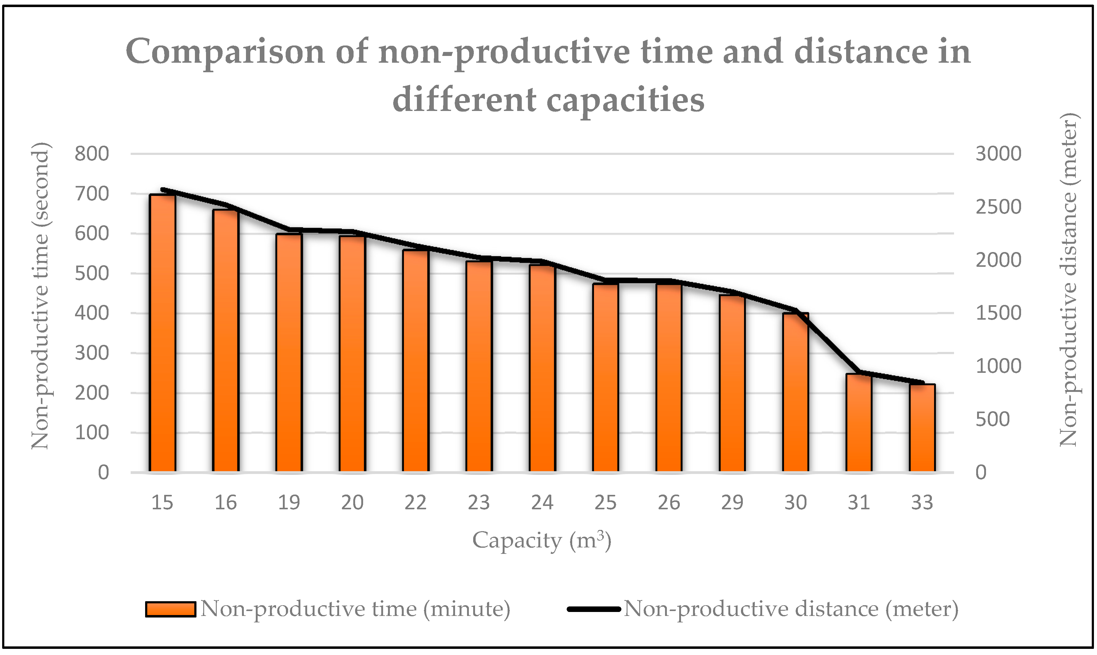
In order to make a strategic decision about the optimal capacity of the slurry distributor, the optimization and simulation model was applied to a range of capacities to find out in which capacity there is an optimal solution for the target field and the amount of non-working time/distance calculated for those solutions.

Table 9. The results of the optimal solution for possible capacities.

Capacity of Slurry Tank (L)	Weight (tons)	Non-Productive Time (min)	Non-Productive Distance (m)	Required Tractor’s Power Take Off (PTO) (hp)
15,000	18	11.6344	2667	180
16,000	19.2	11.002	2522	200
19,000	22.8	9.9852	2289	240
20,000	24	9.9066	2271	260
22,000	26.4	9.3193	2136	280
23,000	27.6	8.841	2026	300
24,000	28.8	8.6836	1990	300
25,000	30	7.9044	1812	320
26,000	31.2	7.8946	1809	340
29,000	34.8	7.433	1704	380
30,000	36	6.6692	1529	380
31,000	37.2	4.1349	948	400
33,000	39.6	3.6942	847	420

presents the average values of running the optimization and simulation model for five times for each possible capacity. The non-working time and distance were calculated based on the location of the field’s gate.

The following diagram (Figure 10) shows the values of non-productive time and distance related to each capacity that the optimization algorithm has found a solution for that. The comparison demonstrates that the capacity equal to 33 (m³) has less non-working time and distance as compared to the other options.

Two more factors, the weight of the slurry tank and the required amount of tractor’s horsepower for pulling the distributor were considered to make a better decision for choosing the proper capacity of the slurry tanker. Indeed, the weight of the distributer affects the soil compaction, and in turn, conceivably the crop yield [31,32,33]. To generalize this problem, the weighted sum model (WSM) [34] method was applied. According to this method, when there are $m$ alternatives and $n$ criteria, the best alternative is the one that satisfies (in the minimization case) the following expression:

$$A_{WSM-score}^{\ast }=\underset{i}{\min }{{\displaystyle \sum }}_{j=1}^n{a}_{ij}{w}_j , for i=1,2,3,\dots ,m.$$

(15)

In this expression, the $A_{WSM-score }^{\ast }$ is the WSM score of the best alternative, $n$ is the number of decision criteria, $a_{ij}$ is the actual value of the $i^{th}$ alternative in terms of the $j^{th}$ criterion, and $w_j$ is the weight of importance of the $j^{th}$ criterion.

According to Table 9, there are 13 alternatives and 4 criteria and the only things that need to be defined are the weight of each criterion. In this study, the significance of the criteria defined as the following matrix (

Table 10. The weight matrix (non-productive distance: the highest significance).

Weight (tons)	Non-Productive Time (min)	Non-Productive Distance (m)	Required Tractor PTO (hp)
$W_1$	$W_2$	$W_3$	$W_4$
2	3	4	1

):

For simplicity, the values of Table 9 can be normalized before calculating the amount of $A_{WSM-score }^{\ast }$. Calculation shows that $A_{WSM-score }^{\ast }$ equal to 5.223 related to the capacity 33,000 L is the minimum score among all the alternatives. Therefore, based on the defined weights in Table 10, the proper capacity to cover the target field is 33,000 L.

Based on the defined significance of the criteria by the farmer, the selected capacity can change. For instance, if the soil compaction get the highest weight and the weight matrix changes as follow: (W1 = 4, W2 = 1, W3 = 2, W4 = 3), as a result, the value of $A_{WSM-score }^{\ast }$ would be equal to 6.104 which is the score of the capacity 15,000 L. Moreover, if we consider the same weight for all the criteria equal to one then, the proper capacity would be 31,000 L with the score equal to 2.603.

4. Discussion

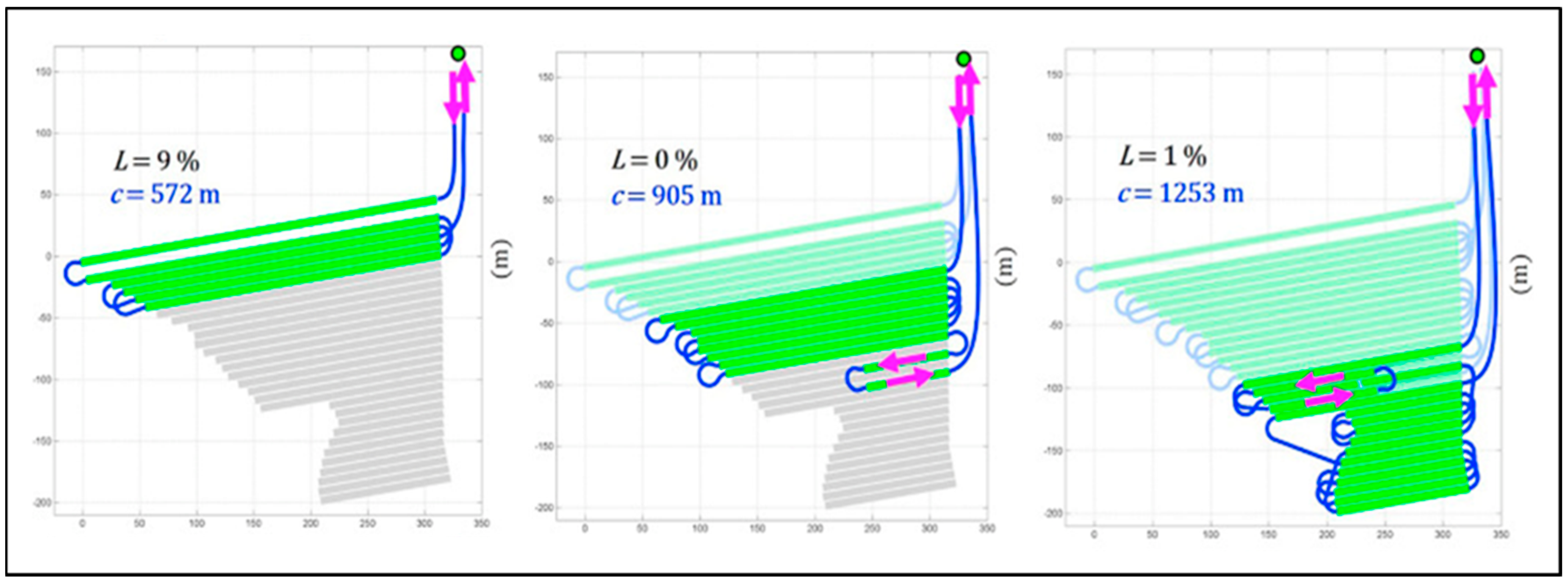
Coverage planning for capacitated operation (such as fertilization) is presented in other studies [22,35]. In order to compare the presented method in this study with other techniques, another approach for coverage planning of capacitated field operations was considered to show the advantages or drawbacks of the proposed approach. According to the study by [26] (Jensen, Bochtis, and Sørensen, 2015), they applied an algorithmic approach for the optimization of liquid fertilizing operation. Their method is based on the state-space search and the output solution is a sequence of pre-defined driving actions to change an initial state to a goal state by minimizing the non-working traveled distance in the target field. The soil injection fertilizing operation A was considered in this part for comparison. All the input data regarding the operation A were presented in the following table (

Table 11. Information regarding the fertilizing operation A.

Location	$\mathbf{Tan}\mathbf{k}\mathbf{Capacity}\left({\mathit{m}}^3\right)$	Working Width (m)	Dosage (t/ha)	Number of Tracks	Turning Radius (m)
Latitude: 55°29’19” N Longitude: 11°59’32” E	25	7.5	17	30	9

).

Figure 11 demonstrates the optimized coverage plan for operation A. Based on the results, the total amount of non-productive distance can be determined by accumulating the non-working distance for each route, equal to 2730 m.

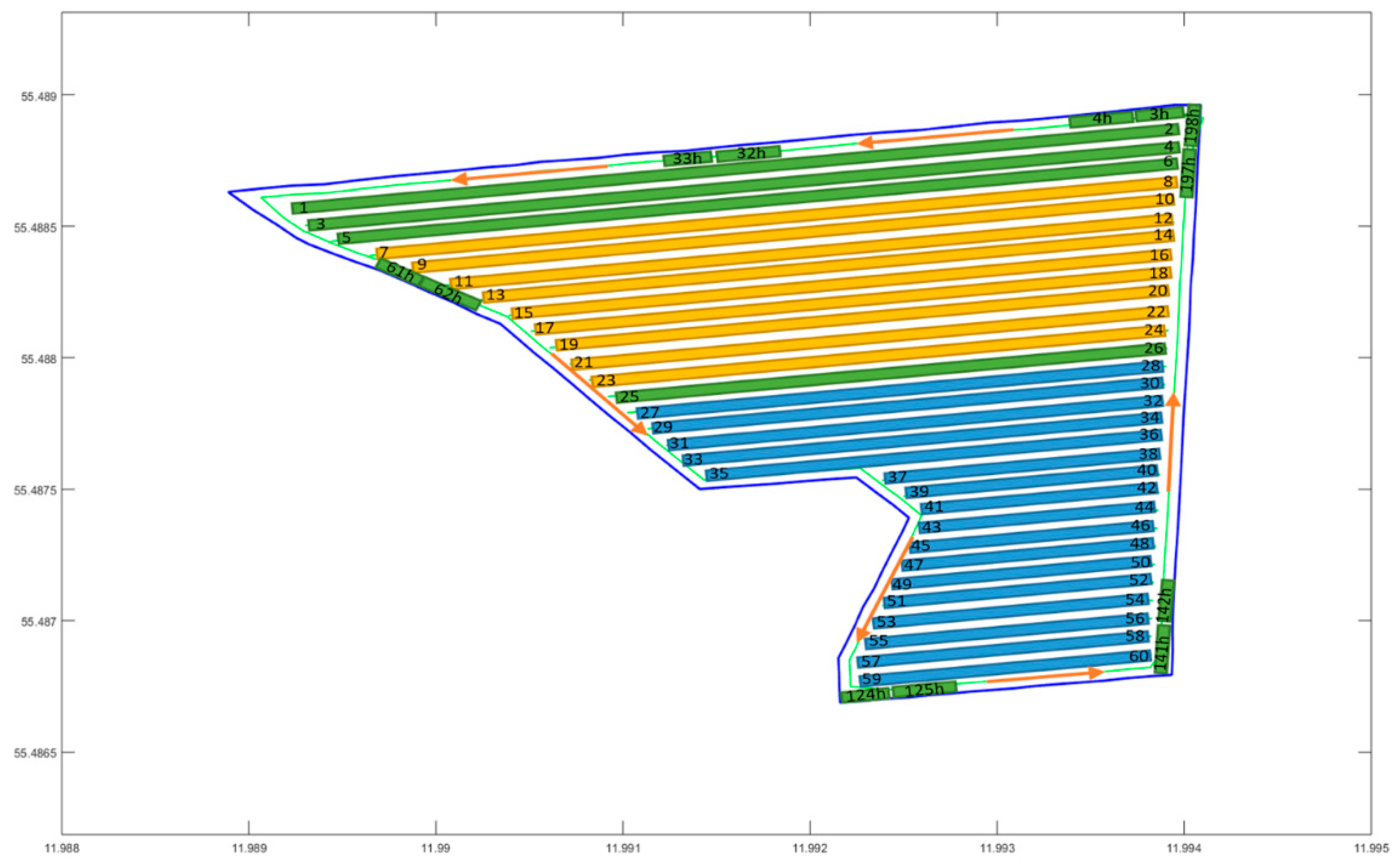
The information presented in Table 11 was applied in the optimization and simulation model as input data and as a result, an optimized solution generated and provided in the following table (

Table 12. The optimized plan for operation A, based on the proposed method in this study.

Optimized Solution	<0, 12, 9, 8, 13, 20, 21, 24, 17, 16, 0, 30, 31, 54, 55, 58, 59, 51, 50, 47, 44, 41, 40, 45, 36, 37, 34, 27, 0, 4, 1, 6, 25, 3 h, 4 h, 5 h, 6 h, 7 h, 8 h, 9 h, 10 h, 11 h, 12 h, 13 h, 14 h, 15 h, …, 198 h, 199 h, 0>
Non-Working Distance (m)	2788

). Moreover, the list of optimized application rate for all the work rows generated and demonstrated in

Table A2. List of application rates for operation A.

Node/Edge ID	Application Rate (L/m2)	Node/Edge ID	Application Rate (L/m2)
1	1.439959	86 h	1.43994
4	1.439959	87 h	1.439942
6	1.439959	88 h	1.439989
8	1.599644	89 h	1.439958
9	1.599644	90 h	1.439965
12	1.599644	91 h	1.439978
13	1.599644	92 h	1.440023
16	1.599644	93 h	1.439989
17	1.599644	94 h	1.439952
20	1.599644	95 h	1.439937
21	1.599644	96 h	1.439989
24	1.599644	97 h	1.439981
25	1.439959	98 h	1.44
27	1.721439	99 h	1.439989
30	1.721439	100 h	1.439959
31	1.721439	101 h	1.439927
34	1.721439	102 h	1.439989
36	1.721439	103 h	1.439955
37	1.721439	104 h	1.439967
40	1.721439	105 h	1.439963
41	1.721439	106 h	1.43996
44	1.721439	107 h	1.439985
45	1.721439	108 h	1.439963
47	1.721439	109 h	1.439968
50	1.721439	110 h	1.43997
51	1.721439	111 h	1.439975
54	1.721439	112 h	1.439972
55	1.721439	113 h	1.439939
58	1.721439	114 h	1.439967
59	1.721439	115 h	1.439931
3 h	1.440067	116 h	1.439964
4 h	1.439989	117 h	1.439948
5 h	1.439989	118 h	1.439949
6 h	1.439951	119 h	1.439972
7 h	1.439945	120 h	1.439955
8 h	1.439989	121 h	1.439954
9 h	1.43996	122 h	1.439951
10 h	1.439894	123 h	1.439888
11 h	1.439948	124 h	1.439945
12 h	1.439989	125 h	1.439949
13 h	1.439961	126 h	1.439974
14 h	1.439948	127 h	1.439974
15 h	1.439941	128 h	1.439942
16 h	1.439973	129 h	1.439959
17 h	1.439989	130 h	1.439966
18 h	1.439948	131 h	1.439989
19 h	1.439976	132 h	1.43996
20 h	1.439952	133 h	1.439964
21 h	1.439948	134 h	1.439966
22 h	1.439908	135 h	1.439959
23 h	1.439969	136 h	1.439958
24 h	1.439989	137 h	1.439964
25 h	1.439967	138 h	1.439955
26 h	1.439935	139 h	1.439967
27 h	1.439948	140 h	1.439967
28 h	1.439978	141 h	1.439958
29 h	1.439959	142 h	1.439989
30 h	1.439948	143 h	1.43996
31 h	1.439941	144 h	1.439966
32 h	1.439972	145 h	1.439973
33 h	1.439989	146 h	1.439964
34 h	1.439948	147 h	1.439976
35 h	1.43999	148 h	1.439989
36 h	1.439987	149 h	1.439993
37 h	1.439989	150 h	1.439949
38 h	1.439948	151 h	1.439926
39 h	1.439996	152 h	1.439957
40 h	1.439942	153 h	1.439959
41 h	1.439989	154 h	1.440004
42 h	1.439944	155 h	1.439945
43 h	1.439958	156 h	1.439952
44 h	1.439948	157 h	1.440043
45 h	1.439989	158 h	1.439968
46 h	1.439968	159 h	1.439962
47 h	1.439964	160 h	1.439934
48 h	1.439948	161 h	1.439948
49 h	1.439948	162 h	1.439947
50 h	1.43995	163 h	1.439969
51 h	1.439948	164 h	1.439989
52 h	1.439941	165 h	1.439996
53 h	1.439952	166 h	1.439955
54 h	1.439989	167 h	1.439953
55 h	1.439965	168 h	1.439963
56 h	1.439915	169 h	1.439955
57 h	1.439948	170 h	1.439964
58 h	1.440012	171 h	1.439957
59 h	1.439963	172 h	1.439961
60 h	1.439948	173 h	1.439958
61 h	1.439946	174 h	1.43997
62 h	1.439957	175 h	1.43996
63 h	1.439948	176 h	1.439964
64 h	1.439986	177 h	1.439964
65 h	1.439933	178 h	1.439966
66 h	1.43994	179 h	1.439963
67 h	1.43996	180 h	1.439954
68 h	1.439961	181 h	1.439963
69 h	1.439946	182 h	1.439967
70 h	1.439949	183 h	1.439963
71 h	1.43997	184 h	1.439961
72 h	1.439944	185 h	1.43996
73 h	1.439958	186 h	1.439957
74 h	1.439943	187 h	1.439964
75 h	1.439949	188 h	1.439965
76 h	1.439968	189 h	1.439966
77 h	1.439969	190 h	1.439953
78 h	1.439972	191 h	1.43996
79 h	1.43996	192 h	1.43996
80 h	1.439948	193 h	1.439955
81 h	1.439985	194 h	1.439953
82 h	1.43994	195 h	1.439946
83 h	1.439953	196 h	1.439989
84 h	1.439938	197 h	1.439948
85 h	1.439989	198 h	1.439942

in Appendix A part. The amount of traveled non-working distance based on the presented method in this study is slightly (58 m) more than the approach provided by [26] (Jensen, Bochtis, and Sørensen, 2015). However, the presented solution in this study avoids all the turning through the main crop area of the field, and in this way, there is less soil compaction in comparison with the method provided by [26] (Jensen, Bochtis, and Sørensen, 2015). Figure 12 shows the optimized coverage plan for operation A based on the proposed method in this study.

5. Conclusions

A coverage-planning algorithm was developed for capacitated field operations such as slurry applications in agricultural fields. The meta-heuristic algorithm simulated annealing (SA) was applied to find the optimal traversal sequence of fieldwork tracks under the criterion of minimizing the non-working traveled distance during the headland turnings together with an adapted application rate for each track. Furthermore, a simulation model was developed to generate the segmentation of the task time and traveled distance for each element (productive/non-productive) of the operation.

The operations efficiency of the optimized plans generated by the proposed method in this paper were compared with conventional non-optimized methods used by farmers. The results showed that applying this new method could accomplish 18.6% and 28.1% reduction in the non-working traveled distance and the non-working time, respectively.

The proposed algorithm could be used as part of a tool to support strategic decisions about the capacity of the machine in capacitated operations such as slurry applications. Four factors (the weight of slurry tanker, non-productive time/distance, and required tractor’s hp) were considered for comparison between different capacities to find the proper one.

Future research will focus on a method to find the optimal coverage plan for a target field by specific configurations of the machine (such as capacity). In this case, the algorithm will be able to find an optimal coverage plan for a sample field with any defined capacity of the slurry tank.

References

- Sørensen, C.; Jacobsen, B.; Sommer, S. An Assessment Tool applied to Manure Management Systems using Innovative Technologies. Biosyst. Eng. 2003, 86, 315–325. [Google Scholar] [CrossRef]
- Sørensen, C. Technologies and logistics for handling, transport and distribution of animal manures. In Animal Manure Recycling: Treatment And Management, 1st ed.; Sommer, S.G., Christensen, M.L., Schmidt, T., Stoumann Jensen, L., Eds.; John Wiley & Sons Ltd.: Chichester, West Sussex, UK, 2013; pp. 211–236. [Google Scholar]
- Huijsmans, J. Effect of application method, manure characteristics, weather and field conditions on ammonia volatilization from manure applied to arable land. Atmos. Environ. 2003, 37, 3669–3680. [Google Scholar] [CrossRef]
- Jensen, M.; Nørremark, M.; Busato, P.; Sørensen, C.; Bochtis, D. Coverage planning for capacitated field operations, Part I: Task decomposition. Biosyst. Eng. 2015, 139, 136–148. [Google Scholar] [CrossRef]
- Edwards, G.; Jensen, M.; Bochtis, D. Coverage planning for capacitated field operations under spatial variability. Int. J. Sustain. Agric. Manag. Inform. 2015, 1, 120. [Google Scholar] [CrossRef]
- Hameed, I.; la Cour-Harbo, A.; Osen, O. Side-to-side 3D coverage path planning approach for agricultural robots to minimize skip/overlap areas between swaths. Robot. Auton. Syst. 2016, 76, 36–45. [Google Scholar] [CrossRef]
- Bochtis, D.; Vougioukas, S. Minimising the non-working distance travelled by machines operating in a headland field pattern. Biosyst. Eng. 2008, 101, 1–12. [Google Scholar] [CrossRef]
- Bochtis, D.; Sørensen, C. The vehicle routing problem in field logistics part I. Biosyst Eng. 2009, 104, 447–457. [Google Scholar] [CrossRef]
- Rodias, E.; Berruto, R.; Busato, P.; Bochtis, D.; Sørensen, C.; Zhou, K. Energy Savings from Optimised In-Field Route Planning for Agricultural Machinery. Sustainability 2017, 9, 1956. [Google Scholar] [CrossRef] [Green Version]
- Bochtis, D.; Sørensen, C.; Busato, P.; Berruto, R. Benefits from optimal route planning based on B-patterns. Biosyst Eng. 2013, 115, 389–395. [Google Scholar] [CrossRef]
- Ho, W.; Ho, G.; Ji, P.; Lau, H. A hybrid genetic algorithm for the multi-depot vehicle routing problem. Eng. Appl. Artif. Intell. 2008, 21, 548–557. [Google Scholar] [CrossRef]
- Toth, P.; Vigo, D. The Vehicle Routing Problem; Society for Industrial and Applied Mathematics: Philadelphia, PA, USA, 2002. [Google Scholar]
- Shen, J.; Shigeoka, K.; Ino, F.; Hagihara, K. GPU-based branch-and-bound method to solve large 0-1 knapsack problems with data-centric strategies. Concurr. Comput. Pract. Exp. 2018, 31. [Google Scholar] [CrossRef]
- Cao, C.; Li, C.; Yang, Q.; Zhang, F. Multi-Objective Optimization Model of Emergency Organization Allocation for Sustainable Disaster Supply Chain. Sustainability 2017, 9, 2103. [Google Scholar] [CrossRef] [Green Version]
- Yuliza, E.; Puspita, F. The Branch and Cut Method for Solving Capacitated Vehicle Routing Problem (CVRP) Model of LPG Gas Distribution Routes. Sci. Technol. Indones. 2019, 4, 105. [Google Scholar] [CrossRef] [Green Version]
- Pamosoaji, A.; Dewa, P.; Krisnanta, J. Proposed Modified Clarke-Wright Saving Algorithm for Capacitated Vehicle Routing Problem. Int. J. Ind. Eng. Eng. Manag. 2019, 1, 9. [Google Scholar] [CrossRef]
- Simultaneous Multi-Start Simulated Annealing for Capacitated Vehicle Routing Problem. WSEAS Trans. Comput. Res. 2020, 8. [CrossRef]
- Chokanat, P.; Pitakaso, R.; Sethanan, K. Methodology to Solve a Special Case of the Vehicle Routing Problem: A Case Study in the Raw Milk Transportation System. AgriEngineering 2019, 1, 75–93. [Google Scholar] [CrossRef] [Green Version]
- Sbai, I.; Limam, O.; Krichen, S. An effective genetic algorithm for solving the capacitated vehicle routing problem with two-dimensional loading constraint. Int. J. Comput. Intell. Stud. 2020, 9, 85. [Google Scholar] [CrossRef]
- Akbar, M.; Aurachmana, R. Hybrid genetic–tabu search algorithm to optimize the route for capacitated vehicle routing problem with time window. Int. J. Ind. Optim. 2020, 1, 15. [Google Scholar] [CrossRef] [Green Version]
- Kanso, B. Hybrid ANT Colony Algorithm for the Multi-depot Periodic Open Capacitated Arc Routing Problem. Int. J. Artif. Intell. Appl. 2020, 11. [Google Scholar] [CrossRef] [Green Version]
- Bochtis, D.; Sørensen, C.; Green, O. A DSS for planning of soil-sensitive field operations. Decis. Support Syst. 2012, 53, 66–75. [Google Scholar] [CrossRef]
- Oksanen, T.; Visala, A. Coverage path planning algorithms for agricultural field machines. J. Field Robot. 2009, 26, 651–668. [Google Scholar] [CrossRef]
- Spekken, M.; de Bruin, S. Optimized routing on agricultural fields by minimizing maneuvering and servicing time. Precis. Agric. 2012, 14, 224–244. [Google Scholar] [CrossRef]
- Ali, O.; Verlinden, B.; Van Oudheusden, D. Infield logistics planning for crop-harvesting operations. Eng. Optim. 2009, 41, 183–197. [Google Scholar] [CrossRef] [Green Version]
- Jensen, M.; Bochtis, D.; Sørensen, C. Coverage planning for capacitated field operations, part II: Optimisation. Biosyst. Eng. 2015, 139, 149–164. [Google Scholar] [CrossRef]
- Overview of the Danish Regulation of Nutrients in Agriculture; Ministry of Agriculture and Food in Denmark: Copenhagen, Denmark, 2017.
- Python Programming Language. Python Software Foundation. Available online: https://www.python.org (accessed on 1 April 2020).
- Conesa-Muñoz, J.; Bengochea-Guevara, J.; Andujar, D.; Ribeiro, A. Route planning for agricultural tasks: A general approach for fleets of autonomous vehicles in site-specific herbicide applications. Comput. Electron. Agric. 2016, 127, 204–220. [Google Scholar] [CrossRef]
- MATLAB® Technical Programming Language; The MathWorks, Inc.: Natick, MA, USA, 1994–2020.
- Gasso, V.; Sørensen, C.; Oudshoorn, F.; Green, O. Controlled traffic farming: A review of the environmental impacts. Eur. J. Agron. 2013, 48, 66–73. [Google Scholar] [CrossRef]
- Keller, T.; Sandin, M.; Colombi, T.; Horn, R.; Or, D. Historical increase in agricultural machinery weights enhanced soil stress levels and adversely affected soil functioning. Soil Tillage Res. 2019, 194, 104293. [Google Scholar] [CrossRef]
- Raper, R. Agricultural traffic impacts on soil. J. Terramech. 2005, 42, 259–280. [Google Scholar] [CrossRef]
- Budiharjo, A.; Muhammad, A. Comparison of Weighted Sum Model and Multi Attribute Decision Making Weighted Product Methods in Selecting the Best Elementary School in Indonesia. Int. J. Softw. Eng. Its Appl. 2017, 11, 69–90. [Google Scholar] [CrossRef]
- Bochtis, D.; Sørensen, C.; Green, O.; Moshou, D.; Olesen, J. Effect of controlled traffic on field efficiency. Biosyst. Eng. 2010, 106, 14–25. [Google Scholar] [CrossRef]