Estimating Plant Pasture Biomass and Quality from UAV Imaging across Queensland’s Rangelands


1
Grazing Land Systems/Remote Sensing Centre, Queensland Department of Environment and Science, Eco-sciences Precinct, Dutton Park, Brisbane 4102, Queensland, Australia
2
Joint Remote Sensing Research Centre, University of Queensland, St Lucia, Brisbane 4072, Queensland, Australia
3
International Centre for Applied Climate Sciences, University of Southern Queensland, Toowoomba 4350, Queensland, Australia
*
Author to whom correspondence should be addressed.
AgriEngineering 2020, 2(4), 523-543; https://0-doi-org.brum.beds.ac.uk/10.3390/agriengineering2040035
Submission received: 27 September 2020
/
Revised: 24 October 2020
/
Accepted: 30 October 2020
/
Published: 5 November 2020
(This article belongs to the Special Issue Digital Agriculture: Latest Advances and Prospects)
Abstract
:The aim of this research was to test recent developments in the use of Remotely Piloted Aircraft Systems or Unmanned Aerial Vehicles (UAV)/drones to map both pasture quantity as biomass yield and pasture quality as the proportions of key pasture nutrients, across a selected range of field sites throughout the rangelands of Queensland. Improved pasture management begins with an understanding of the state of the resource base, UAV based methods can potentially achieve this at improved spatial and temporal scales. This study developed machine learning based predictive models of both pasture measures. UAV-based structure from motion photogrammetry provided a measure of yield from overlapping high resolution visible colour imagery. Pasture nutrient composition was estimated from the spectral signatures of visible near infrared hyperspectral UAV sensing. An automated pasture height surface modelling technique was developed, tested and used along with field site measurements to predict further estimates across each field site. Both prior knowledge and automated predictive modelling techniques were employed to predict yield and nutrition. Pasture height surface modelling was assessed against field measurements using a rising plate meter, results reported correlation coefficients () ranging from 0.2 to 0.4 for both woodland and grassland field sites. Accuracy of the predictive modelling was determined from further field measurements of yield and on average indicated an error of 0.8 t ha−1 in grasslands and 1.3 t ha−1 in mixed woodlands across both modelling approaches. Correlation analyses between measures of pasture quality, acid detergent fibre and crude protein (ADF, CP), and spectral reflectance data indicated the visible red (651 nm) and red-edge (759 nm) regions were highly correlated (ADF R2 = 0.9 and CP R2 = 0.5 mean values). These findings agreed with previous studies linking specific absorption features with grass chemical composition. These results conclude that the practical application of such techniques, to efficiently and accurately map pasture yield and quality, is possible at the field site scale; however, further research is needed, in particular further field sampling of both yield and nutrient elements across such a diverse landscape, with the potential to scale up to a satellite platform for broader scale monitoring.
1. Introduction
Queensland’s rangelands occupy over 80% of the state and are extensively grazed by sheep and cattle, estimates in excess of 20 million exist [1]. The value of this industry to the state and national economy is estimated at over $5 billion per-annum [2]. Native pastures account for the majority of the feed-base of this industry. The climate of these native pastures is highly variable. The initial antecedent climatic conditions, including the existing soil, water and pasture growth state, is an often-overlooked aspect of systems thinking for managing climate variability [3]. This simple concept provides the starting point to any future projection of productivity driven by how the future seasonal climate may unfold. Even if no formulated forecast position is taken, and median conditions (climatology) or persistence of the current situation might be assumed, any future projection of pasture growth still requires a current system state. Pasture resource assessment, that is current pasture biomass (growing, senescing and dead), pasture quality and grazing land condition, is the key to setting sustainable livestock numbers. Describing the ambient antecedent condition of Queensland pasture resources is problematic due to the heterogeneous nature of grazing landscapes at micro and macro spatial scale over the year.
Queensland has one of the most variable climates in the world, frequented by episodic droughts, floods, wildfires and tropical cyclones [4]. This highly variable climate results in a wide range of seasonal pasture production of varying quality. Therefore, the matching of livestock numbers to the available pasture resource requires continual observation and fine-tuning of herbivore density [1,5]. Overgrazing of the pasture resource results in loss of grass cover, development of bare patches of ground which can become highly erodible, unfavourable changes in palatable pasture species composition and phenotype and increases in woody vegetation [6]. The effect of degradation causes a loss in productivity and potentially more overgrazing to compensate, further development of erosion gullies from accelerated runoff and loss of sediment into waterways and in some cases into the Great Barrier Reef lagoon [7].
The estimation of stocking rates depends on the assessment of the available and future pasture biomass and its quality. There are various methods for making these assessments, including (1) manual collections of pasture biomass along defined transects using quadrat harvests or estimations [8], (2) collecting well-calibrated rising-plate measurements also along established transects [9], (3) optical satellite-based observations such as Landsat, Sentinel and Modis [10], (4) through simulation modelling of pasture production, hybrid satellite-pasture simulation approaches [11], and more recently, (5) drones or UAVs used to assess pasture growth and pasture quality [12,13]. Benefits and limitations exist with all techniques, but UAVs whether alone or in fusion with other techniques promise to be a major enabling technology. The scientific literature over the past few years shows emerging benefits from UAV-captured photogrammetric, multispectral and hyperspectral imaging of pasture condition with examples from the USA, Brazil, Europe, Australia and South Africa [13,14,15,16]. An optimum solution using data fusion possibly exists, combining the best aspects of all technologies. Support of the simulation can be bolstered by incorporation of satellite-based remote sensing imagery and local field measurements; however, achieving sufficient calibration observations over a large area requires intensive field data. The introduction and evolution of sophisticated drone or UAV platforms are a great promise for bridging this gap. For example, UAVs can observe at centimetre resolution with photogrammetric, multispectral and hyperspectral techniques.
This study aims to build upon recent advancements in UAV technologies, to develop and test a method to map and monitor pasture resources across the large and heterogeneous rangelands of Queensland, Australia. It aims to be a method that can be applied at a range of spatial and temporal scales as an important component of both long-term broad-scale pasture monitoring programs, as well as a stand alone or complimentary onground decision support tool. It aims to do this by way of developing similar measures of pasture yield and nutrient composition to that of traditional plot based field sampling techniques in a more efficient and spatially explicit manner. This will improve integration into satellite-derived products to scale beyond the extents of a field site as a key component to broad scale monitoring and reporting. In addition, onground decision makers will also be able to precisely assess the state of the pasture resource at a finer submetre spatial resolution, building further confidence in remotely sensed data. Improved confidence and adoption of satellite derived pasture resource estimations through access and use of finer scale UAV imagery and associated pasture state estimations, aims to provide the necessary tools for setting more sustainable long-term livestock numbers by graziers.
Pasture biomass estimation from a UAV platform is a relatively new technique. To date the majority of published research has been undertaken in other countries in either improved or cultivated pastures. Natural pastures in Australia remain largely under-studied. UAV photogrammetry Structure from Motion (SfM) is one of two methods used to determine vegetation height, the other being Light Detection and Ranging (LiDAR). LiDAR uses laser technology in an active manner to measure the distances from the device to the object, whereas photogrammetry SfM is a method of measuring height and mass from many overlapping photographs [17]. Pasture biomass has been mostly determined from the latter technique as it is a considerably less expensive technology and pastures are more likely to be in environments that are not obstructed by other vegetation such as tall or dense tree canopies. Linear modelling of the relationship between pasture height and biomass is a well established method [18,19]. Modelling of this relationship with UAV SfM is becoming more popular and several studies have reported strong correlation between UAV derived imagery and ground-based estimates. [13,14] reported average values as high as 0.78 and 0.81 in both the native pastures of Arizona, USA and a cultivated pasture in northern Germany. This case study over a number of dominant grasslands and woodlands of the rangelands of Queensland, attempted to develop a similar technique that, as previously stated, could be both used to potentially cross calibrate satellite imagery for broader applications across the rangelands of Queensland and as a standalone measure of pasture biomass at the field, paddock and property scales for improved pasture management.
Sustainable livestock grazing, through improved matching of stocking rates to pasture resources, depends not only on the amount of pasture biomass but importantly both its species composition and nutrient status. Adequate crude protein in the diet of livestock is essential for their maintenance, growth, lactation and reproduction [20]. Pasture digestibility becomes limiting to livestock growth and reproduction when it reaches certain levels. Acid detergent fibre (ADF) is an inverse measure of pasture digestibility. The importance of crude protein in livestock diets has been studied for many decades [21]. The use of remote sensing, field and laboratory spectroscopy is also well established in the literature [22,23,24]. Pasture nutrient status is a field of study that has recently re-emerged since the development and affordability of UAV technologies. In comparison to past airborne/satellite and field based systems, UAV hyperspectral remote sensing provides a more cost-effective and spatially explicit means of measuring known plant chemical components. Such components are useful as indicators of pasture nutrition and digestibility for livestock grazing. Crude protein and ADF are two commonly used indicators of pasture digestion. Recent UAV studies have demonstrated the use of hyperspectral sensing in detecting both crude protein and ADF in the natural pastures of other countries [15]. UAV hyperspectral sensors are not low-cost; however, for nutrient estimation they are essential. The aim of this study will be to demonstrate the use of UAV hyperspectral remote sensing to detect both crude protein and ADF in a range of native pastures across the rangelands of Queensland.
Study Area
The study area illustrated in Figure 1a encompasses most of Queensland’s rangelands, an area of approximately one million square kilometres. It is a mix of both dry tropical to subtropical rangelands in the north and along the coast and arid to semiarid rangelands throughout the interior. Annual average rainfall ranges from 1800 mm on the north east coast down to 1400 mm on the south east coast and 1000 mm in the north west interior to below 200 mm in the south west interior [25]. Field sites were established in a mix of woodland and grassland communities to sample a range of pasture biomass, heights and nutrient compositions. Sites in each community were further stratified to characterise both rainfall gradients and pasture compositions. Table 1 details the number of sites in each community and category along with the dates of each field sampling campaign. Figure 1a illustrates the location and spatial distribution of the field sites across the study area. Figure 1b also presents examples of several field sites seen through high-resolution UAV imagery, illustrating the mixtures of vegetation composition, structure and pasture biomass.
2. Materials and Methods
2.1. Field Site Sampling
Nineteen field sites were established using the methods and protocols developed by [26]. Each field site encompassed an area of approximately one hectare, within which three 100 m transects were established. Pasture biomass was sampled from eighteen individual 0.25 m2 quadrats, placed adjacent to each transect at set intervals of 15 metres apart. Prior to pasture biomass removal, a rising plate meter was used to record pasture height (PHrp) in mm at the centre of each 0.25 m2 sample quadrat. The Jenquip EC20TM Bluetooth electronic plate-meter was used to record pasture height along with the open-source Open-Data-Kit (ODK) app to collect and send the field data, for management and storage, to the Australian Terrestrial Ecosystem Research Network field-data database [27]. All standing herbaceous vegetative material was removed by electric shears to a height of approximately 2 cm above the ground. Each individual quadrat sample was placed into a bar-coded paper bag, the GPS location recorded, a pre and post cut photograph taken and the sample bag scanned using the ODK app. Each sample was then oven-dried for a period of 72 h at 65 degrees Celsius and then weighed to determine Total Standing Dry Matter (TSDM) in tonnes per hectare (t ha−1) per each 0.25 m2 sample quadrat. TSDM samples were further processed to determine nutrient composition. All eighteen quadrat samples from each field site were first combined, mixed and a subsample extracted. Subsamples were ground through a 2mm screen using a centrifugal mill. Each subsample was then sent for traditional chemistry analysis at the University of Queensland—School of Agriculture and Food Science laboratory. Firstly organic matter and ash content of each sample was determined after combustion at 550 degrees Celsius for eight hours. The percent of ash-free Acid Detergent Fibre (ADF) was then determined using an Ankom fibre digestion unit, using procedures described by the manufacturer. Percent crude protein was then determined using the methods developed by [28]. Laboratory processing was only conducted on a subset of 10 grassland sites, 8 of which were located in the Mitchell grasslands and 2 in the arid grasslands.
2.2. UAV Data Capture
2.2.1. Mission Planning and Execution
UAV imagery was collected at each field site following the establishment of ground control targets, sampling transects and quadrats but prior to field measurements. The UgCS mission planning software version 2.0TM was used to program each autonomous flight. The average flight mission parameters and the equipment used for both photogrammetric and hyperspectral missions are detailed in Table 2. All flights were conducted between the hours of 10:00 to 14:00 h local time to reduce shadowing and each campaign was flown in clear to minimal cloud.
2.2.2. Ground Control
Submetre geographic position and elevation accuracy of each UAV capture was achieved by way of the deployment of Ground Control Point (GCP) targets across each field site. Each GCP consisted of a Propeller AeroPointTM ground control point that was used in the correction of UAV imagery. A minimum of four hours of differential GPS data was collected for each target, submetre accuracy of each target was achieved through either correction to the Propeller AeroPointTM network, or where it was not available, each target was corrected to a Septentrio Altus NR3TM GNSS receiver that was established as a base-station for each survey. The base-station position was established through the Australian AUSCORS network [29] online processing tool. The GCP positions utilising the Propeller correction network was assessed against established coordinates for a field site. A Leica TS50TM robotic total station along with Topcon HiPer SRTM GNSS receivers were used to conduct a combined GNSS and terrestrial observation survey of each of eight GCP targets to a precision of less than 0.6 mm + 1 ppm distance and 0.5 (Hz&V) angular measurements.
2.3. Data Processing and Analysis
2.3.1. UAV DSLR RGB Imagery
Image processing of the DSLR RGB images was performed with the Pix4D commercial software [30]. As [31] states, numerous studies have assessed this software for the generation of surface modelling and the estimation of plant height, including [32,33]. Ref. [31] further explains the use of computer vision methods including Structure-from-Motion (SfM) for the automated/simultaneous estimation of the interior and exterior orientation parameters and coordinates of a sparse point cloud from many overlapping individual images. This study employed such techniques including the integration of ground control targets as an important component for planimetry and altimetry accuracy [34] in [31]. Applying the SfM methods in Pix4D with the RGB images and GCP targets a Digital Surface Model (DSM) was generated over each field site. The processing parameters and resources are presented in Table 3 and the steps involved are summarised in Figure 2. Pasture height () was next calculated as the difference between each DSM elevation pixel value and the minimum surrounding elevation value, that aims to represent the ground surface elevation. A moving window of a set size was used to determine the value of each window’s central focus pixel. An appropriate window size was determined through testing the linear relationships of each field site’s rising plate measurements () with their calculated for many window sizes. A maximum window size of five metres was chosen, as beyond this the slope of the site was assumed to influence an accurate measurement of . The correlation coefficient of each incremented window size from one centimetre up to five metres was calculated in single pixel increments. The highest coefficient was then used to determine the optimum window size for each field site. Processing of large window sizes is computationally resource intensive, the python package geo-wombat [35] employs a number of parallel and block processing tools that were tested and successfully deployed on both a Linux based high performance compute facility and a standalone alone high-specification desktop PC. Maximum was next extracted from each field site’s individual quadrats across each image and matched with the same field and measurements. The strength of the relationship was then tested through least squares linear modelling. Maximum was chosen to closely match that of the rising plate measure settling height. This was carried out in a GIS by way of identifying each quadrat in the UAV orthomosaic image of each field site. A polygon around each quadrat was manually digitised then utilised to extract the maximum height values of each quadrat from each field site surface image. In the instance that an individual quadrat was occluded or partially occluded by tree or shrub cover, it was excluded from further analysis. Quadrats that were identified to be in the shadow of associated tree and shrub cover were not excluded from further analyses.
2.3.2. UAV Hyperspectral Imagery
The ReSe PARGETM orthorectification and the Harris ENVITM image analysis software were used to perform image correction, orthorectification and atmospheric calibration of each UAV hyperspectral imaging campaign. To begin with the Corning MicroHSITM hyperspectral sensors onboard dark target calibration and Non-Uniformity Correction (NUC) was applied to each raw scan by default. Further image processing utilised the NUC corrected imagery. Next, each scan was imported into the PARGE software and an orthorectification completed. Pixel-wise direct geo-referencing was conducted based on the interpolation of the sensors onboard coordinate position, elevation and attitude information for each scan-line position in a parametric geo-coding approach. The input and output parameters of the rectification are detailed in Table 3. Radiometric calibration was next carried out to further reduce atmospheric effects and derive relative surface reflectance () from the orthorectified data cube. Areas of flat homogeneous reflectance in the imagery were determined from an ASD handheld2TM AVNIR spectrometer. The surfaces of the Propeller AeroPointsTM ground control point targets were tested and determined to be suitable flat spectra. Using the ENVI image analysis software Region of Interest (ROI) tool the orthorectified image spectra across the surface of each GCP target was sampled and used in the flat field normalisation procedure in ENVI. The surface reflectance value of each image pixel was calculated according to Equation (1).
where i, j and represent image row, column and band; DN is the microHSI sensor dark target and NUC corrected digital number and WR is the aero-point white reference target averaged spectral value.
Spectra from each field site’s individual quadrat were next sampled from the imagery in a similar manner to that of the normalisation target selection. The field sampled pastures within each quadrat were digitised as polygons with the ROI tool. A false colour near-infrared colour composite of the imagery was produced to enable interpretation of pastures from background soils and other nonvegetative material. The average spatial spectral response from all 18 quadrat polygons for each spectral band was calculated and matched to the same laboratory measured proportions of acid detergent fibre and crude protein, for further statistical analysis. Each stage in the hyperspectral image processing is further summarised in Figure 2.
2.4. Statistical Analysis
2.4.1. Pasture Biomass
Two approaches to estimating pasture biomass through predictive modelling were developed and compared. The first approach utilised a selected statistical model based on prior knowledge of its suitability to the modelling task. The second utilised an automated process, termed “automatic ML” or automated machine learning. The first approach involved the use of a Random Sample Consensus (RANSAC) robust linear regression modelling technique. The aim of this method is to improve the fit of the model based on subsets of the data that is determined as inliers and outliers. It was chosen based on its performance with noisy data problems [36]. The second automatic ML approach involved the use of the Tree-based Pipeline Optimisation Tool (TPOT). TPOT is a python automated machine learning tool that optimises machine learning pipelines using genetic programming [37]. A number of input parameters are chosen to initialise the TPOT process and are summarised in Table 4. The default TPOT ten fold cross-validation procedure using a 75/25 split was employed to train and test 10,000 model configurations to find the most suitable model and its associated parameters.
Preprocessing of both the interdependent variable and dependant variable involved an assessment of potential erroneous outliers. This involved calculation of each variable’s Z-score or signed number of standard deviations above or below its mean value. A filter of 2.5 deviations was set and those records above and below were flagged for further error assessment. The TSDM harvest weight of each identified quadrat, along with the associated field sites pasture and landscape variables, i.e., dominant vegetation and soil types, was used to select a corresponding pasture standard photograph from an archive of available pasture photograph standards [38]. The matching standard photograph was then compared with the quadrat photograph taken prior to harvest, a visual assessment of the likelihood of the quadrat photograph matching the standard photograph and its associated yield was made and the quadrat record either removed from further analysis or included. Matching photographs in this manner was only indicative as the standard photographs were taken at an oblique angle and the quadrat photographs in a nadir position above each quadrat, where the visual error assessment was not obvious the record was not excluded from further analysis. A total of 12 samples were removed from further analysis in this manner from an overall sample of 242 records. Further preprocessing of the dependant variable included its normalisation using the Box & Cox power transformation [39]. Following both modelling procedures, an evaluation of each was performed. A Monte-Carlo simulation, similar to the resampling technique evaluated by [40], was run for several thousand iterations, with each iteration randomly selecting training and testing data sets. In each iteration the model developed from both RANSAC and the TPOT optimisation was fitted with 75% of the data and a prediction tested with the remaining 25%. The Root Mean Square Error (RMSE) of each iteration of each model was calculated and stored. The distribution of the overall RMSE from all of the iterations was then used to illustrate the stability of both modelling processes and the variability of the methods ability to predict . As an illustration of the two modelling processes, each output model was then applied to an independent grassland field sites image and the spatially averaged of the image across each sample quadrat compared to the average field sampled values.
2.4.2. Pasture Nutrient Estimation
In a similar approach to [15], correlation analysis was first conducted to determine the relationship between ADF and CP in the field sampled with that of the corresponding sampled spectra. Normalisation of was carried out using the vector transformation of Equation (2) [15] where is the spectral vector for i = 1, 2,..., n.
The first derivative of the normalisation function was also calculated as a means of potentially revealing further spectral characteristics. The spectral ratio (SR) and normalisation difference spectral indices (NDSI) were calculated as additional metrics to be tested for correlation with the field measurements of pasture quality. Least-squares linear regression modelling was then used to test the correlation. The coefficient of determination values of both the transformations and spectral features and the original spectra, were then used to determine the optimal method, ratio or indices, based on the highest average correlation coefficient value. Following the correlation analysis, further statistical modelling was constrained by the limited sampling size of only 10 field site pasture quality measurements. The aim of this study was to explore the application of the methods developed by [15] to identify similar wavelength correlations with the same pasture quality measures in a landscape of very different vegetation to their study. The same robust regression modelling procedure used in the pasture yield modelling of this study was next applied to the imagery of an independent Mitchell grassland field site in the study area. Based on the results of the correlation analysis, the most suitable wavelength was selected and used to model both pasture quality measures across the field site.
3. Results
3.1. Ground Control Accuracy
The accuracy of the Propeller AeroPointTM GCP’s utilising their base station network solution was tested against a combined GNSS/terrestrial theodolite survey. Results of the survey and discrepancies between them and their estimated position and elevation are presented in Table 5.
3.2. Field Site Sample Results
Results of both pasture biomass yield and wet chemistry analyses are illustrated in Figure 3. Pasture yield has been grouped by vegetation subcategory, biomass is highest for the Mitchell grassland category with an average of 1.5 t ha−1 and lowest 0.4 t ha−1 for the Arid grasslands. Yield of the two woodland categories were 1.4 t ha−1 and 0.8 t ha−1. Pasture nutrient analyses are presented by individual grassland field sites Figure 3b. Protein is relatively low across all sites with an average of only 9%. Differences between sites is also low with an average of only 1%. Acid detergent fibre is, however, distinctively different with a much higher overall average of 41% and a higher average difference of 4% between field sites.
3.3. Pasture Height Comparisons
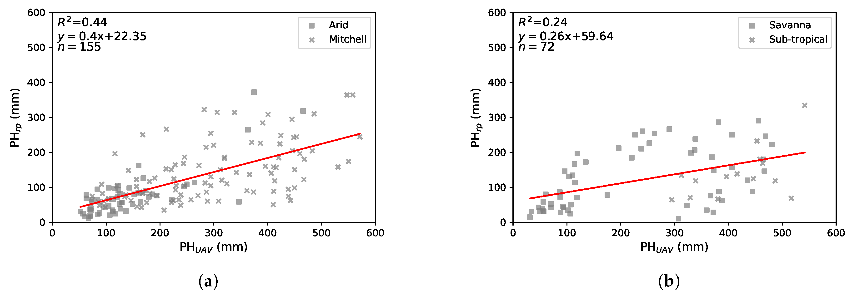
Comparisons of a linear least-squares regression between and are illustrated for all four subcategories in Figure 4. The two woodland subcategories had the lowest levels of precision with an overall value of 0.24. The two grassland subcategories demonstrated higher precision with an overall precision of 0.44. The linear relationship between and decreased as height increased for both broad categories. Individual measurements in the majority of cases were less than that of their associated measurement. Figure 5 illustrates some of the constraints of the pasture height modelling method including occlusion and shadowing of individual sample quadrats by tree and shrub cover.
3.4. Predictive Modelling
3.4.1. Pasture Biomass
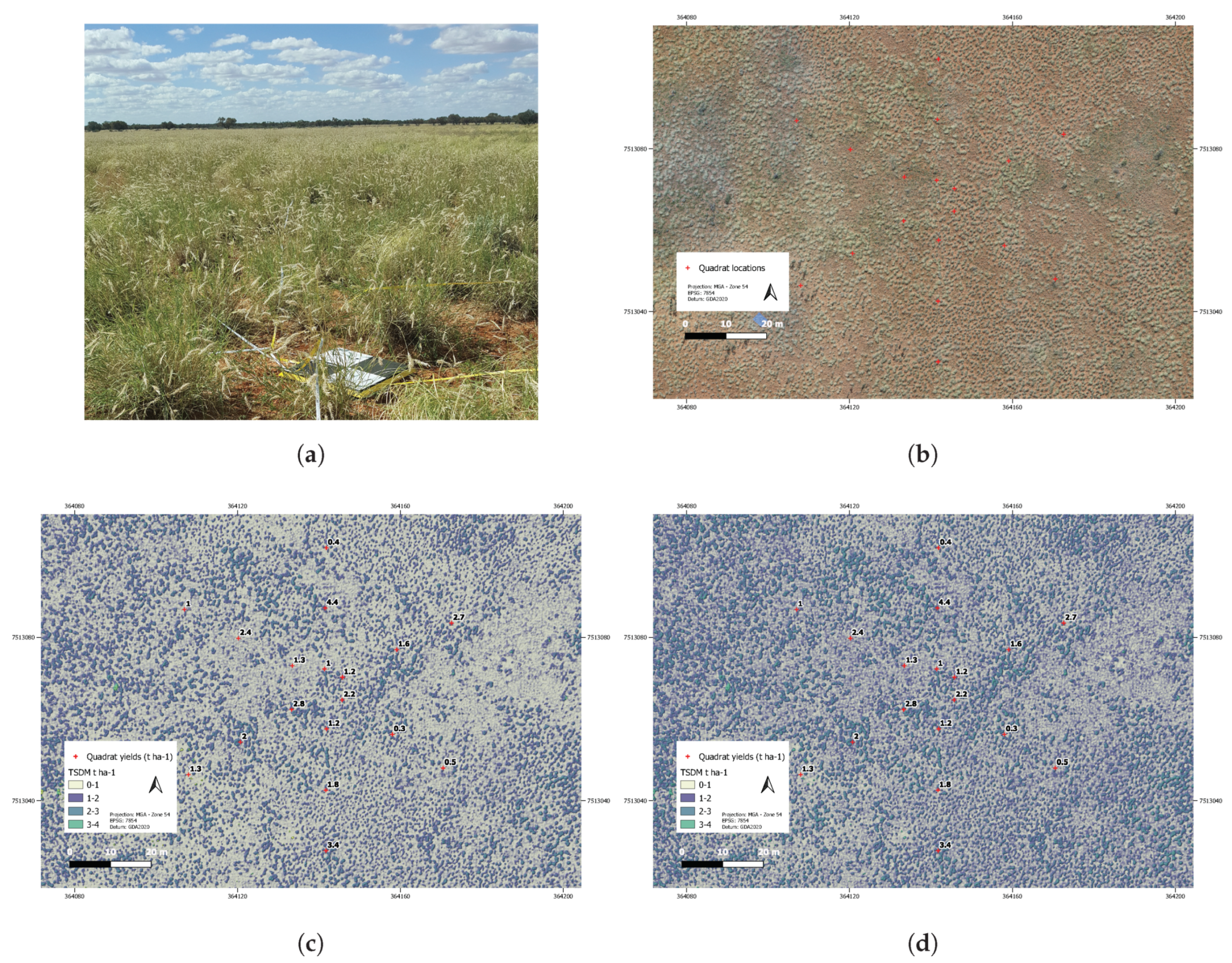
The application of both modelling procedures to an independent field site is first illustrated in Figure 6. Plate (a) provides a photograph of the field site illustrating the pastures of the site from an oblique perspective and map (b), an orthomosaic image of the site from the photogrammetry survey, provides an aerial perspective. Map (c) illustrates the automated ML model and map (d) the robust regression model. Slight differences can be seen between the models whereby map (d), the robust regression model has a higher overall yield. This is confirmed in comparing the field measured yields against each modelled yield. The automated ML TSDM yield was calculated on average across all 18 quadrats at 0.96 t ha−1 compared to the field measured average TSDM of 1.84 t ha−1. The robust regression was in comparison closer to the field measurement at 1.23 t ha−1, a difference of only 0.61 t ha−1.
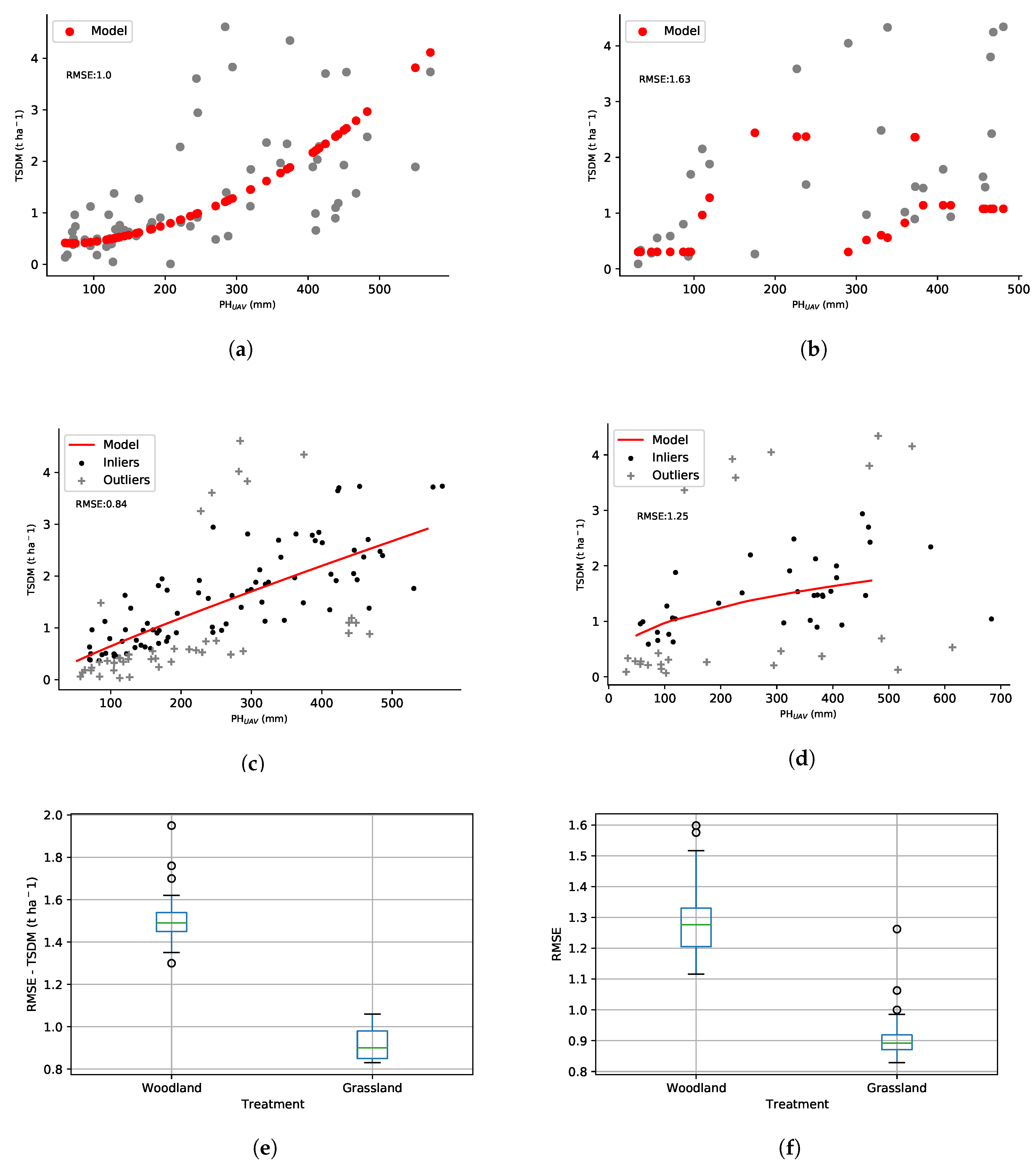
The results of both the prior knowledge robust regression model and automated ML learning procedure are next presented. The automated ML procedure resulted in the selection of an XGB regressor model for the woodlands training data set and a SGD regressor model for the grassland training data set. The results of the testing data set are next presented in Figure 7. The automated ML models have a slighter higher RMSE error and therefore lower accuracy than the robust regression modelling, as seen in both the individual plots of each model for each category (a–d) and in the results of the accuracy assessment (e and f). The accuracy of both modelling procedures is higher for the grassland category than the woodland and in the case of the woodland automated ML algorithm, model overfitting has occurred as seen in Figure 7b.
3.4.2. Pasture Quality
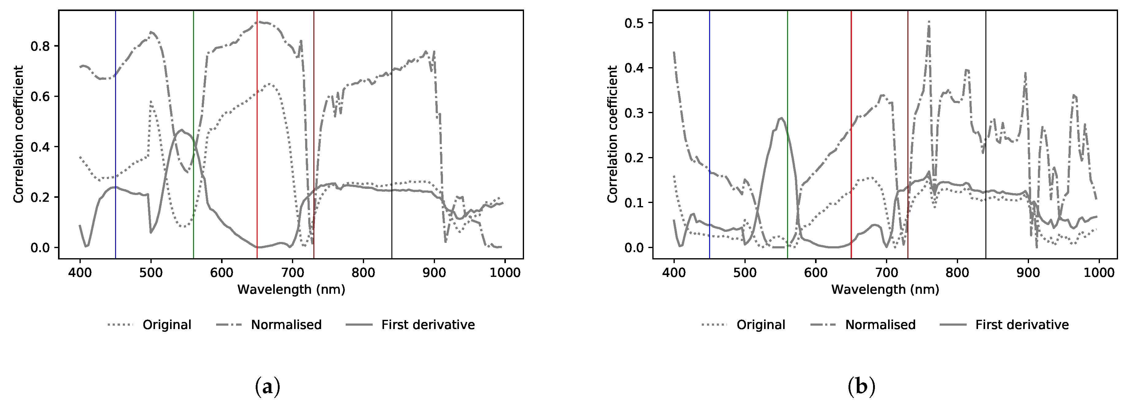
The results of the correlation of each of the 150 spectral bands with that of the field sampled acid detergent fibre and crude protein are presented in the form of a correlogram. Figure 8 illustrates these relationships and Table 6 further details and identifies the strongest correlations. The normalised transformation appears to have the strongest correlation. The single band, ratio and NDSI index are all relatively similar for each pasture quality measure with the exception of the single band spectral feature for the crude protein measure. Acid detergent fibre has a strong correlation in the visible red portion of the spectrum and crude protein has a distinctive peak past the red edge portion of the spectrum.
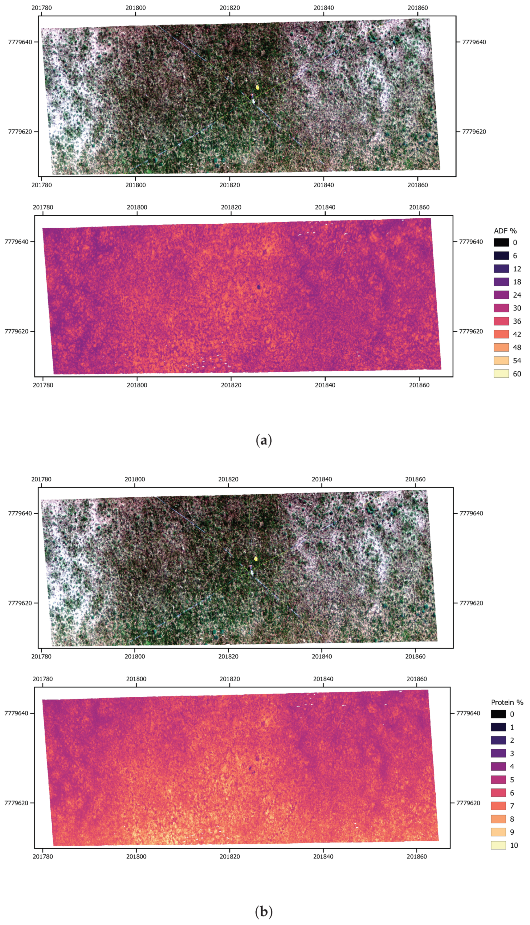
The two example images in Figure 9 illustrate the application of the robust regression modelling to an area of Mitchell grassland utilising the normalised single-band spectral feature for the acid detergent fibre measure and the simple ratio for the crude protein measure. The spatial distribution of both acid detergent fibre and crude protein can be seen across the field site. The crude protein element appears to be visually higher than the acid detergent fibre both in its overall proportion and spatial distribution.
4. Discussion
Survey accurate ground control was important to this study for the matching of field observations with UAV imagery, processing of the SfM photogrammetry and in the orthorectification of the hyperspectral scan imagery. Survey accuracy at each field site varied depending on the base station solution. As described in the methods section the Propeller AeroPointTM network solution was used where it was available, and a portable base station solution, corrected through the AUSCORS network [29], was utilised in more remote locations. Submetre accuracy of both solutions was achieved but likely varied between one another; however, in the absence of an extensive base station network across the vast rangelands of Australia this was still considered an acceptable level of accuracy.
Field sampling of pasture height, yield and quality is not without its own sampling error. Previous studies have used other methods such as terrestrial laser scanning and hand-held spectroscopy [22,41], although these methods were initially trialled in this study, a simple and direct means of collecting field measurements was chosen. Limitations of each method exist, in this study these included the ability of the rising plate method to accurately measure pasture height across rough and undulating ground surfaces, often resulting in erroneous pasture heights due to the rising plate base not accurately contacting with the true ground surface. Pasture yield harvesting of TSDM also has limitations, including the ability to physically harvest low sample sizes such as in arid and sparse grasslands. Other limitations in sampling efforts included the amount of samples collected that would adequately represent the variability of each metric in both their statistical and spatial distributions. Limitations in time and resources meant a smaller overall field sample set was collected than would likely be needed to definitively model each metric across the diverse range of landscapes of the study area. However, this research was able to demonstrate the applicability of the various field sampling techniques and methods to both compare and calibrate the UAV-borne imagery and associated metrics.
The UAV pasture height model () was compared with the rising plate field measurements () (see Figure 4). Results of the comparisons across all four pasture subcategories illustrate the potential of this method. Both grassland categories showed on average a strong correlation in the lower pasture height range that weakened as height increased. This was also present in the woodland categories, however not as distinctively. Pasture heights of most grasslands of the study area were relatively low, on average less than 70 cm tall. Taller pasture may become problematic using the rising plate field measurement method. A number of limitations of the method were discovered. The presence of tree and shrub-cover limits the ability to accurately determine the pasture sward height both in the physical obstruction or occlusion of the pasture sward by tree and/or shrub canopy cover as well as the effects of shadowing from the canopy layer and its effects on the calculation of the elevation and pasture height surfaces. An example of such a field site is illustrated in Figure 5 and the degree of these effects upon the accurate determination of both and the resultant modelled TSDM t ha−1 estimates is seen in both the robust and automated ML modelling outputs. In the case of the automated ML output, spurious estimates of have resulted in an overfitting of the model. The robust regression modelling approach, however, is able to exclude some of these potential outliers and provide a better fit. Further to this limitation, the chosen window size used in determining the ground surface elevation has a significant impact on the overall accuracy of the surface. An iterative process was chosen whereby the strength of the correlation of and was used to determine the most suitable window size. Although this showed potential, its practical application may be limited, particularly in the problematic landscapes for accurate measurement. Automated ground layer determination is problematic in high resolution photogrammetry based digital elevation or terrain modelling, particularly in finer scale (<5 cm) imagery. Numerous tree and forestry based point cloud filtering methods exist, including [42,43]; however, application at a finer scale becomes computationally resource intensive. This becomes further problematic in dense pastures of sloping terrain, whereby a true measure of the ground surface elevation is difficult to determine for each pixel. Several recent studies such as [13,31] have physically selected and/or surveyed ground surface elevations used in the calculation of a digital terrain model to then determine the pasture or canopy height surface. This approach was considered impractical in this study and problematic in the often sloping terrains of the study area. Although a number of limitations exist in the field and UAV measurement of pasture height exist, a least-squares linear regression of both the field and UAV derived measures in this study indicated the potential of the UAV based method to replace the manual method, with enough ongoing validation across a range of pasture heights, swards and species.
The ability to develop accurate UAV based models of pasture yield have been demonstrated in this study. The estimation of pasture yield or biomass was explored with both a prior knowledge robust regression modelling approach and an automatic machine learning method. Both approaches proved successful with reasonable levels of accuracy. The robust regression approach performed slightly better, likely due to its ability to deal with some of the before mentioned erroneous field measurements through its classification and weighting of statistical outliers. Although this approach could potentially reduce valid outliers, it was deemed a useful technique. The stratification of the field measurements of pasture yield and the development of separate models for both woodland and grassland pasture groups improved each model’s performance. The grassland model performed better than the woodland, likely the result of the before mentioned limitations of modelling pasture height in mixed tree and grassland pastures. The robust regression again performed better than the auto ML model in both the grassland and woodland separate models. This was particularly evident in the woodland group whereby overfitting of the model occurred as discussed previously. The accuracy assessments of each modelling method and its associated stratification shows a similar trend in that the variability of the accuracy of each model increases for the woodland group and to some degree the auto ML method. Improvements to the auto ML modelling method’s output accuracy could include optimisation and potentially weighting models in the selection procedure to include those with advanced procedures in removing or weighting outliers. The calibration of further predictive modelling of pasture yield will likely need further field measurements. The models developed in this study provide a basis for further modelling.
High correlation between specific bands of the UAV hyperspectral imaging with that of the proportions of acid detergent fibre and crude protein, in predominantly the Mitchell grassland pastures of the study area, has been demonstrated in this study. In a study with similar pastures, [22] reported crude protein absorption features of a moist grassland in South Africa, to be in the wavelength range between 720 to 745 nm of the red edge portion of the spectrum. This study reported a similar distinctive peak in correlation of the single-band spectral feature at 759.85 nm (see Figure 8). However, this study reported a stronger correlation with both the simple-ratio and normalised index at the 939.92 and 947.92 nm portions of the spectrum, also referred to as the third overtone absorption mechanism [44], whereby plant tissue oil and protein compounds are absorbed; however, it is more commonly associated with the short wave near infrared portion of the spectrum. Regression of acid detergent fibre was also different to [22] but similar to [15] in that the best correlation was in the visible portion of the spectrum for the single-band spectral feature, specifically visible red at 651.81 nm. The visible red (651.81 nm) and protein absorption/near-infrared portions (919.91 and 939.92 nm) illustrated the highest correlation for the simple ratio and normalised index. These results, although slightly dissimilar to other studies with similar techniques, illustrate the potential for further research utilising these techniques, into the pastures of the study area. In particular, these results show the sensitivities of this type of visible near infra-red hyperspectral imaging to accurately estimate the proportions of crude protein and acid detergent fibre in the pastures of the study area in differing growth stages and/or states of pasture decay or senescence, whereby the short-wave near-infrared portion of the spectrum has been more commonly used.
A number of difficulties in accurately mapping both measures were encountered including the successful orthorectification of UAV hyperspectral imagery. Although an area that covered the majority of each field site in a single scan was used in the analysis, subsequent adjacent scans were not, due to difficulties in accurately aligning each scan. Onboard post processing differential GPS position data that can be matched to the hyperspectral sensors IMU positioning is a potential solution to improve the geometric accuracy of each flight scan. Further sensor spectral calibration is the other consideration for ongoing mapping efforts. The UAV hyperspectral sensor used in this study was factory calibrated and will likely need recalibration to ensure spectral measurements are of the highest grade. Only 10 field samples were used to develop a robust regression model of both pasture quality measures; these samples were, however, across a vast geographic range of similar mostly native rangeland pastures and provides a basis for further research. Demonstration of the modelling across an area of Mitchell grassland captured with the same hyperspectral sensor used in this study, provides a basis for further work. This includes the development and testing of further modelling to predict changes in both crude protein and ADF under differing pasture management regimes and pasture growth stages. Ongoing research and development from this initial case study will provide innovative and improved predictions of pasture quality to further develop, inform and improve sustainable grazing decision-making systems.
5. Conclusions and Further Work
The aim of this study was to develop an accurate and spatially explicit measure of pasture biomass and nutrient composition that can be used for both scaling up to satellite-borne imagery for long term broad scale pasture resource monitoring as well as a fine scale measure for improved onground pasture resource management. A number of challenges still exist as already discussed; previous studies using similar techniques have mostly been undertaken in cropped pastures. This study has demonstrated that these techniques can be applied with rigour across the rangelands of Queensland, providing further opportunities to both integrate UAV imaging into satellite-derived products and importantly as standalone measures of real-time pasture state at the paddock and potentially property scales. Improved spatial and temporal measures of pasture state, utilising the methods developed in this study, provide new opportunities for improved pasture management. The existing GRASP pasture growth simulation modelling, developed by [45] and implemented across Queensland’s rangelands by [46], has traditionally utilised point based measurements of climate and pasture state. Integration of both the field scale measures developed in this study and future satellite integrated measures, could provide a more efficient and spatially explicit system, providing producers with further tools to adopt more resilient and longer-term grazing strategies in an increasingly variable climate.
The limitations found in this study lead to a number of key recommendations for further improvements including; (1) further assessment of potential spatial inaccuracies of a differential GPS solution utilising a portable base station versus the Propeller AeroPointTM correction network and the potential impacts of any differences upon down stream photogrammetry processing, (2) improvements to the orthorectification of hyperspectral image products through the incorporation of onboard UAV post processing differential GPS corrections, (3) testing the suitability and practicality of more sophisticated methods of collecting coincidental field measurements for ongoing UAV pasture model calibration and validation including terrestrial laser scanning and both AVNIR and SWIR field spectroscopy, (4) development and incorporation of a tree and shrub canopy and shadow image segmentation, (5) exploration of further automated methods to efficiently and accurately determine ground elevations in fine-scale photogrammetric digital surface modelling, (6) investigation of improvements to pasture yield modelling through further testing and optimising of automated machine learning techniques and importantly further field sampling in areas of poor model performance, including tall and sparse pastures, and lastly (7) further field sampling of pasture quality measurements to enable further sophisticated pasture quality modelling with a larger data set and in a broader range of pasture types in varying stages of growth.
In addition to specific improvements to the methods used in this study, to more accurately model and map both pasture quantity and quality at the field, paddock and potentially property scales, further development of methods to scale each UAV based measure up to satellite derived imagery is needed. This could begin with high to medium spatial resolution platforms such as the Dove Planet and the Copernicus Sentinel constellations of optical and radar satellites. Scaling from centimetre UAV imagery up to one to 10 metre resolution imagery would provide the first steps in understanding the challenges in integrating both platforms. A number of challenges will likely exist, such as differences in radiometric and geometric calibrations between platforms and the effects these differences may have upon the scaling of measurements from one platform to another. However, such efforts will provide further opportunities to apply accurate and efficient field scale measurements to satellite borne imagery for long term/broader scale monitoring. Similar earth observation studies, including [47,48], have begun to explore UAV to satellite imagery integration and along with this research provide a basis for further development in the native pastures of the Queensland rangelands.
Author Contributions
J.B. conducted the research and wrote the paper. S.P. and P.S. provided support, advice and supervision as PhD advisors of the primary author. All authors have read and agreed to the published version of the manuscript.
Funding
This research received no external funding.
Acknowledgments
The anonymous reviewers for their review and feedback of the manuscript. The owners, their families and staff of the numerous pastoral properties that kindly provided support and access to their properties. Support from the Australian Government Research Training Program Scholarship. Support and funding from the University of Queensland Joint Remote Sensing Research Program. Support and funding from the QLD Department of Environment and Science and the Department of Agriculture and Fisheries—Drought and Climate Adaptation Program, staff at the Eco-sciences Precinct Remote Sensing Centre for assistance, support, training, and advice including: Ken Brook, Christina Jones, Jacqui Willcocks, John Carter, Leo Hardke, Jordan Graesser, Rebecca Trevithick and Robert Denham, and assistance in collecting and management of field data from Rebecca Farrell, Al Healy, Grant Stone and Grant Fraser. The University of Southern Queensland’s International Centre for Applied Climate Sciences for hosting the position of the first author.
Conflicts of Interest
The authors declare no conflict of interest.
References
- Johnston, P.; McKeon, G.; Buxton, R.; Cobon, D.; Day, K.; Hall, W.; Scanlan, J. Managing Climatic Variability in Queensland’s Grazing Lands—New Approaches. In Applications of Seasonal Climate Forecasting in Agricultural and Natural Ecosystems; Springer: Dordrecht, The Netherlands, 2010; Chapter III; pp. 197–226. [Google Scholar]
- Department of Agriculture and Fisheries. Queensland Agriculture Snapshot. 2018. Available online: https://www.publications.qld.gov.au/dataset/state-of-queensland-agriculture-report-june-2014/resource/1c4ac429-da34-464d-845c-f3ad536588f8 (accessed on 1 May 2020).
- Schmoldt, D.L. Building Knowledge-Based Systems for Natural Resource Management, 1st ed.; Springer: Boston, MA, USA, 1996. [Google Scholar]
- McKeon, G.; Hall, W.; Henry, B.; Stone, G.; Watson, I. Pasture Degradation and Recovery in Australia’s Rangelands: Learning from History; Queensland Department of Natural Resources, Mines and Energy: Brisbane, Australia, 2004.
- McKeon, G.M.; Day, K.A.; Howden, S.M.; Mott, J.J.; Orr, D.M.; Scattini, W.J.; Weston, E.J. Northern Australian Savannas: Management for Pastoral Production. J. Biogeogr. 1990, 17, 355–372. [Google Scholar] [CrossRef]
- Pickup, G.; Chewings, V.H. A grazing gradient approach to land degradation assessment in arid areas from remotely-sensed data. Int. J. Remote Sens. 1994, 15, 597–617. [Google Scholar] [CrossRef]
- Bartley, R.; Corfield, J.P.; Hawdon, A.A.; Kinsey-Henderson, A.E.; Abbott, B.N.; Wilkinson, S.N.; Keen, R.J. Can changes to pasture management reduce runoff and sediment loss to the Great Barrier Reef? The results of a 10-year study in the Burdekin catchment, Australia. Rangel. J. 2014, 36, 67–84. [Google Scholar] [CrossRef]
- Mannetje, L.; Haydock, K.P. The dry-weight-rank method for the Botanical analysis of pasture. Grass Forage Sci. 1963, 18, 268–275. [Google Scholar] [CrossRef]
- Stockdale, C.R. Evaluation of techniques for estimating the yield of irrigated pastures intensively grazed by dairy cows. 2. The rising plate meter. Aust. J. Exp. Agric. 1984, 24, 305–311. [Google Scholar] [CrossRef]
- Lugassi, R.; Zaady, E.; Goldshleger, N.; Shoshany, M.; Chudnovsky, A. Spatial and Temporal Monitoring of Pasture Ecological Quality: Sentinel-2-Based Estimation of Crude Protein and Neutral Detergent Fiber Contents. Remote Sens. 2019, 11, 799. [Google Scholar] [CrossRef] [Green Version]
- Wang, J.; Xiao, X.; Bajgain, R.; Starks, P.; Steiner, J.; Doughty, R.B.; Chang, Q. Estimating leaf area index and aboveground biomass of grazing pastures using Sentinel-1, Sentinel-2 and Landsat images. ISPRS J. Photogramm. Remote Sens. 2019, 154, 189–201. [Google Scholar] [CrossRef] [Green Version]
- Viljanen, N.; Honkavaara, E.; Näsi, R.; Hakala, T.; Niemeläinen, O.; Kaivosoja, J. A Novel Machine Learning Method for Estimating Biomass of Grass Swards Using a Photogrammetric Canopy Height Model, Images and Vegetation Indices Captured by a Drone. Agriculture 2018, 8, 70. [Google Scholar] [CrossRef] [Green Version]
- Grüner, E.; Astor, T.; Wachendorf, M. Biomass prediction of heterogeneous temperate grasslands using an SFM approach based on UAV imaging. Agronomy 2019, 9, 54. [Google Scholar] [CrossRef] [Green Version]
- Gillan, J.K.; McClaran, M.P.; Swetnam, T.L.; Heilman, P. Estimating Forage Utilization with Drone-Based Photogrammetric Point Clouds. Rangel. Ecol. Manag. 2019, 72, 575–585. [Google Scholar] [CrossRef]
- Wijesingha, J.; Astor, T.; Schulze-Brüninghoff, D.; Wengert, M.; Wachendorf, M. Predicting Forage Quality of Grasslands Using UAV-Borne Imaging Spectroscopy. Remote Sens. 2020, 12, 126. [Google Scholar] [CrossRef] [Green Version]
- Liu, H.; Dahlgren, R.; Larsen, R.; Devine, S.; Roche, L.; O’ Geen, A.; Wong, A.; Covello, S.; Jin, Y. Estimating Rangeland Forage Production Using Remote Sensing Data from a Small Unmanned Aerial System (sUAS) and PlanetScope Satellite. Remote Sens. 2019, 11, 595. [Google Scholar] [CrossRef] [Green Version]
- Fonstad, M.A.; Dietrich, J.T.; Courville, B.C.; Jensen, J.L.; Carbonneau, P.E. Topographic structure from motion: a new development in photogrammetric measurement. Earth Surf. Process. Landf. 2013, 38, 421–430. [Google Scholar] [CrossRef] [Green Version]
- O’Sullivan, M.; O’Keeffe, W.F.; Flynn, M.J. The Value of Pasture Height in the Measurement of Dry Matter Yield. Ir. J.Agric. Res. 1987, 26, 63–68. [Google Scholar]
- Harmoney, K.R.; Moore, K.J.; George, J.R.; Brummer, E.C.; Russell, J.R. Determination of Pasture Biomass Using Four Indirect Methods. Agron. J. 1997, 89, 665–672. [Google Scholar] [CrossRef]
- Oldham, J.; Smith, T. 7-Protein-energy interrelationships for growing and for lactating cattle. In Protein Contribution of Feedstuffs for Ruminants; Miller, E., Pike, I., Eds.; Butterworth-Heinemann: Oxford, UK, 1982; pp. 103–130. [Google Scholar] [CrossRef]
- Elliott, R.C.; Topps, J.H. Studies of protein requirements of ruminants: 2. Protein requirement for maintenance of three breeds of cattle. Br. J. Nutr. 1963, 17, 549–556. [Google Scholar] [CrossRef] [Green Version]
- Singh, L.; Mutanga, O.; Mafongoya, P.; Peerbhay, K. Remote sensing of key grassland nutrients using hyperspectral techniques in KwaZulu-Natal, South Africa. J. Appl. Remote Sens. 2017, 11, 036005. [Google Scholar] [CrossRef]
- Villamuelas, M.; Serrano, E.; Espunyes, J.; Fernández, N.; López-Olvera, J.R.; Garel, M.; Santos, J.; Parra-Aguado, M.Á.; Ramanzin, M.; Fernández-Aguilar, X.; et al. Predicting herbivore faecal nitrogen using a multispecies near-infrared reflectance spectroscopy calibration. PLoS ONE 2017, 12, e0176635. [Google Scholar] [CrossRef] [PubMed] [Green Version]
- Ramoelo, A.; Cho, M. Explaining Leaf Nitrogen Distribution in a Semi-Arid Environment Predicted on Sentinel-2 Imagery Using a Field Spectroscopy Derived Model. Remote Sens. 2018, 10, 269. [Google Scholar] [CrossRef] [Green Version]
- Bureau of Meteorology. Climate Data Online. 2020. Available online: http://www.bom.gov.au/climate/data/ (accessed on 1 June 2020).
- Muir, J.; Schmidt, M.; Tindall, D.; Trevithick, R.; Scarth, P.; Stewart, J. Field Measurement of Fractional Ground Cover: A Technical Handbook Supporting Ground Cover Monitoring for Australia; Technical Report; The Queensland Department of Environment and Resource Management in collaboration with the Australian Bureau of Agricultural and Resource Economics and Sciences: Canberra, Australia, 2011.
- Terrestrial Ecosystem Research Network. Australian Data Discovery Portal. 2012. Available online: https://portal.tern.org.au/#/adba0b85 (accessed on 1 July 2020).
- Möller, J. Cereals, cereals-based products and animal feeding stuffs – determination of crude fat and total fat content by the Randall extraction method: a collaborative study. Qual. Assur. Saf. Crops Foods 2010, 2, 197–202. [Google Scholar] [CrossRef]
- Geoscience Australia. International GNSS Network. 2020. Available online: http://auscors.ga.gov.au/status/ (accessed on 30 July 2020).
- Pix4D. Pix4Dmapper Software Program. 2020. Available online: https://www.pix4d.com/ (accessed on 28 February 2020).
- Batistoti, J.; Marcato Junior, J.; Ítavo, L.; Matsubara, E.; Gomes, E.; Oliveira, B.; Souza, M.; Siqueira, H.; Salgado Filho, G.; Akiyama, T.; et al. Estimating Pasture Biomass and Canopy Height in Brazilian Savanna Using UAV Photogrammetry. Remote Sens. 2019, 11, 2447. [Google Scholar] [CrossRef] [Green Version]
- Leitão, J.P.; Moy de Vitry, M.; Scheidegger, A.; Rieckermann, J. Assessing the quality of digital elevation models obtained from mini unmanned aerial vehicles for overland flow modelling in urban areas. Hydrol. Earth Syst. Sci. 2016, 20, 1637–1653. [Google Scholar] [CrossRef] [Green Version]
- Malambo, L.; Popescu, S.; Murray, S.; Putman, E.; Pugh, N.; Horne, D.; Richardson, G.; Sheridan, R.; Rooney, W.; Avant, R.; et al. Multitemporal field-based plant height estimation using 3D point clouds generated from small unmanned aerial systems high-resolution imagery. Int. J. Appl. Earth Obs. Geoinf. 2018, 64, 31–42. [Google Scholar] [CrossRef]
- Martínez-Carricondo, P.; Agüera-Vega, F.; Carvajal-Ramírez, F.; Mesas-Carrascosa, F.J.; García-Ferrer, A.; Pérez-Porras, F.J. Assessment of UAV-photogrammetric mapping accuracy based on variation of ground control points. Int. J. Appl. Earth Obs. Geoinf. 2018, 72, 1–10. [Google Scholar] [CrossRef]
- Graesser, J. GeoWombat Python Computer Language Package. 2020. Available online: https://github.com/jgrss/geowombat (accessed on 30 May 2020).
- Meer, P.; Mintz, D.; Rosenfeld, A.; Kim, D.Y. Robust regression methods for computer vision: A review. Int. J. Comput. Vis. 1991, 6, 59–70. [Google Scholar] [CrossRef]
- Olson, R.S.; Bartley, N.; Urbanowicz, R.J.; Moore, J.H. Evaluation of a Tree-Based Pipeline Optimization Tool for Automating Data Science. In Proceedings of the Genetic and Evolutionary Computation Conference 2016; Association for Computing Machinery: New York, NY, USA, 2016; pp. 485–492. [Google Scholar] [CrossRef] [Green Version]
- Department of Agriculture and Fisheries. Pasture Photo Standards. 2020. Available online: https://futurebeef.com.au/knowledge-centre/pasture-photo-standards/ (accessed on 30 June 2020).
- Daimon, T. Box–Cox Transformation. In International Encyclopedia of Statistical Science; Lovric, M., Ed.; Springer: Berlin/Heidelberg, Germany, 2011; pp. 176–178. [Google Scholar] [CrossRef]
- Lyons, M.B.; Keith, D.A.; Phinn, S.R.; Mason, T.J.; Elith, J. A comparison of resampling methods for remote sensing classification and accuracy assessment. Remote Sens. Environ. 2018, 208, 145–153. [Google Scholar] [CrossRef]
- Cooper, S.; Roy, D.; Schaaf, C.; Paynter, I. Examination of the Potential of Terrestrial Laser Scanning and Structure-from-Motion Photogrammetry for Rapid Nondestructive Field Measurement of Grass Biomass. Remote Sens. 2017, 9, 531. [Google Scholar] [CrossRef] [Green Version]
- Muir, J.; Goodwin, N.; Armston, J.; Phinn, S.; Scarth, P. An Accuracy Assessment of Derived Digital Elevation Models from Terrestrial Laser Scanning in a Sub-Tropical Forested Environment. Remote Sens. 2017, 9, 843. [Google Scholar] [CrossRef] [Green Version]
- Meng, X.; Currit, N.; Zhao, K. Ground Filtering Algorithms for Airborne LiDAR Data: A Review of Critical Issues. Remote Sens. 2010, 2, 833–860. [Google Scholar] [CrossRef] [Green Version]
- Ustin, S. Manual Of Remote Sensing/Remote Sensing For Natural Resource Management And Environmental Monitoring; Wiley: Hoboken, NJ, USA, 2004. [Google Scholar]
- Rickert, K.; Stuth, J.; McKeon, G. Modelling Pasture and Animal Production. In Field and Laboratory Methods for Grassland and Animal Production Research; CABI Publishing: New York, NY, USA, 2000; Chapter 3; pp. 29–66. [Google Scholar] [CrossRef]
- McKeon, G.; Ash, A.; Hall, W.; Smith, M.S. Simulation of Grazing Strategies for Beef Production in North-East Queensland. In Applications of Seasonal Climate Forecasting in Agricultural and Natural Ecosystems; Hammer, G.L., Nicholls, N., Mitchell, C., Eds.; Springer: Dordrecht, The Netherlands, 2000; pp. 227–252. [Google Scholar] [CrossRef]
- Puliti, S.; Saarela, S.; Gobakken, T.; Ståhl, G.; Næsset, E. Combining UAV and Sentinel-2 auxiliary data for forest growing stock volume estimation through hierarchical model-based inference. Remote Sens. Environ. 2018, 204, 485–497. [Google Scholar] [CrossRef]
- Navarro, J.A.; Algeet, N.; Fernández-Landa, A.; Esteban, J.; Rodríguez-Noriega, P.; Guillén-Climent, M.L. Integration of UAV, Sentinel-1, and Sentinel-2 Data for Mangrove Plantation Aboveground Biomass Monitoring in Senegal. Remote Sens. 2019, 11, 77. [Google Scholar] [CrossRef] [Green Version]
Figure 1.
Locations of field sites (a), across the study area and their vegetation community and type. High-resolution Unmanned Aerial Vehicles (UAV) imagery examples (b) of each type including the arid grasslands (AG), Mitchell grasslands (MG), subtropical woodlands (STW) and (SW) savanna woodlands.
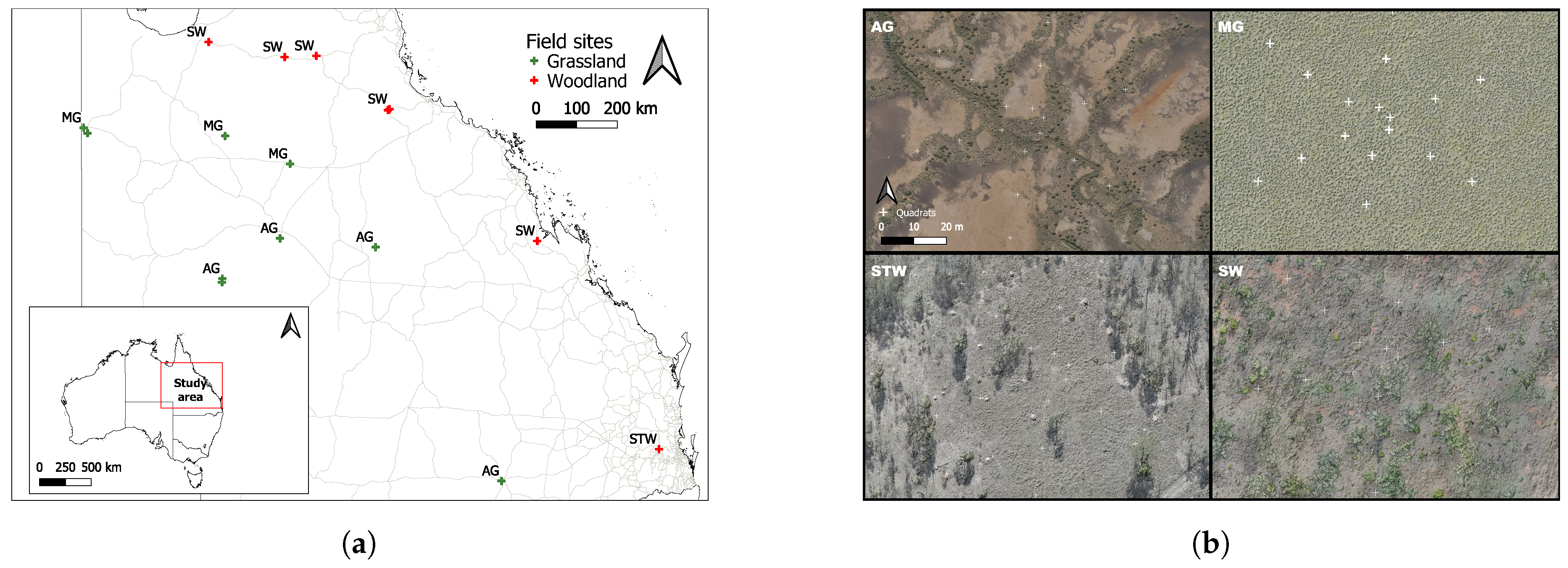
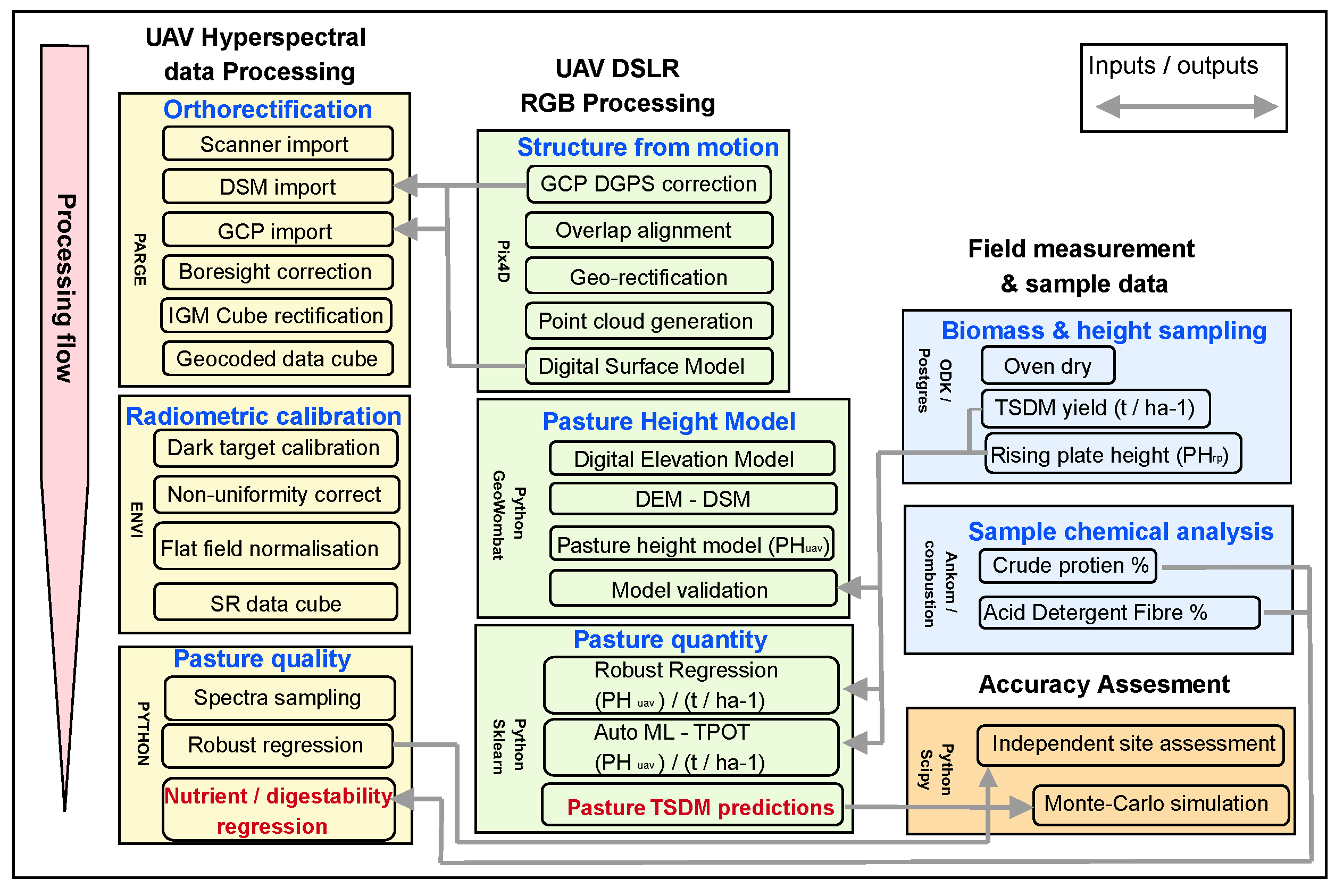
Figure 2.
Flow-diagram of each of the three image and field sample processing streams. Acronyms: DSM—Digital Surface Model, GCP—Ground Control Point, IGM—Input Geometry Method, SR—Surface Reflectance, Auto ML—Automatic Machine Learning, DSLR—Digital Single-lens Reflex camera, TPOT—Tree-based Pipeline Optimisation Tool, TSDM—Total Standing Dry Matter.

Figure 3.
Pasture yield (a) and acid detergent fibre and crude protein laboratory results (b).
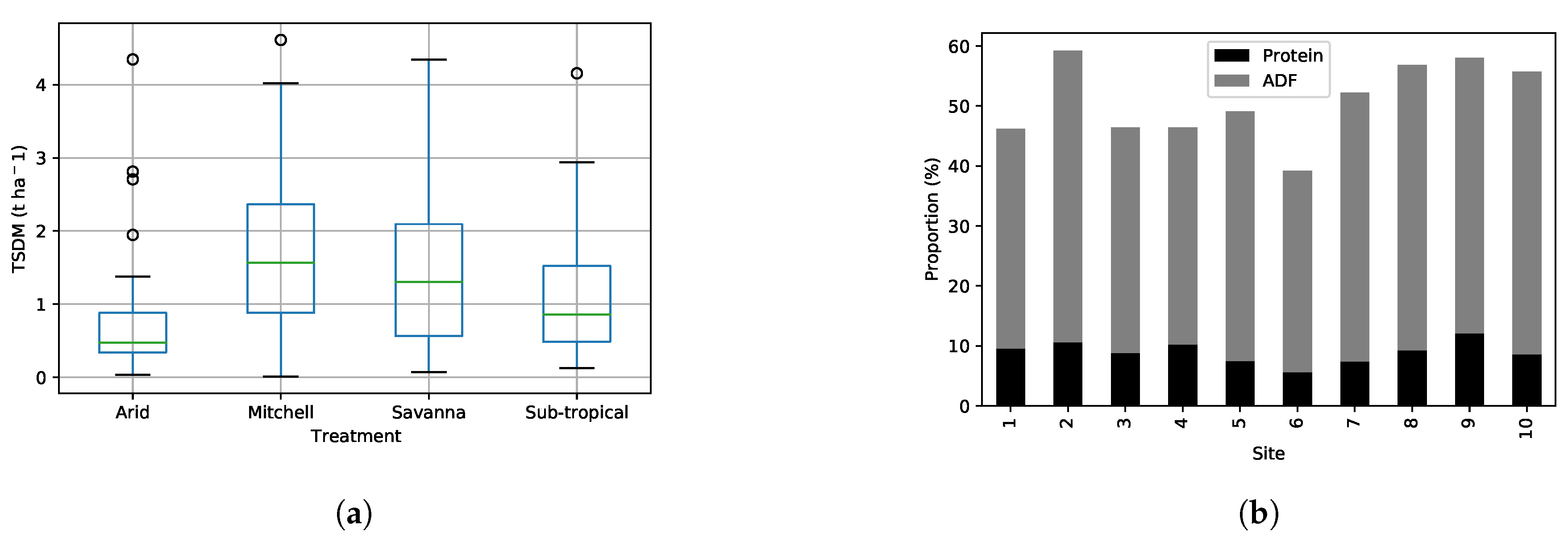
Figure 4.
Least squares linear relationship between pasture height from UAV-based RGB imaging (PHUAV) and manual rising plate meter measurements (PHrp) for both the grassland (a) and woodland (b) categories along with each of their associated subcategories
Figure 4.
Least squares linear relationship between pasture height from UAV-based RGB imaging (PHUAV) and manual rising plate meter measurements (PHrp) for both the grassland (a) and woodland (b) categories along with each of their associated subcategories

Figure 5.
Example orthomosaic imagery of a woodland field site to highlight the extent of tree and shrub cover. Occlusion of the sampling quadrats are illustrated as well as those quadrats that were in shadow at time of capture.
Figure 5.
Example orthomosaic imagery of a woodland field site to highlight the extent of tree and shrub cover. Occlusion of the sampling quadrats are illustrated as well as those quadrats that were in shadow at time of capture.
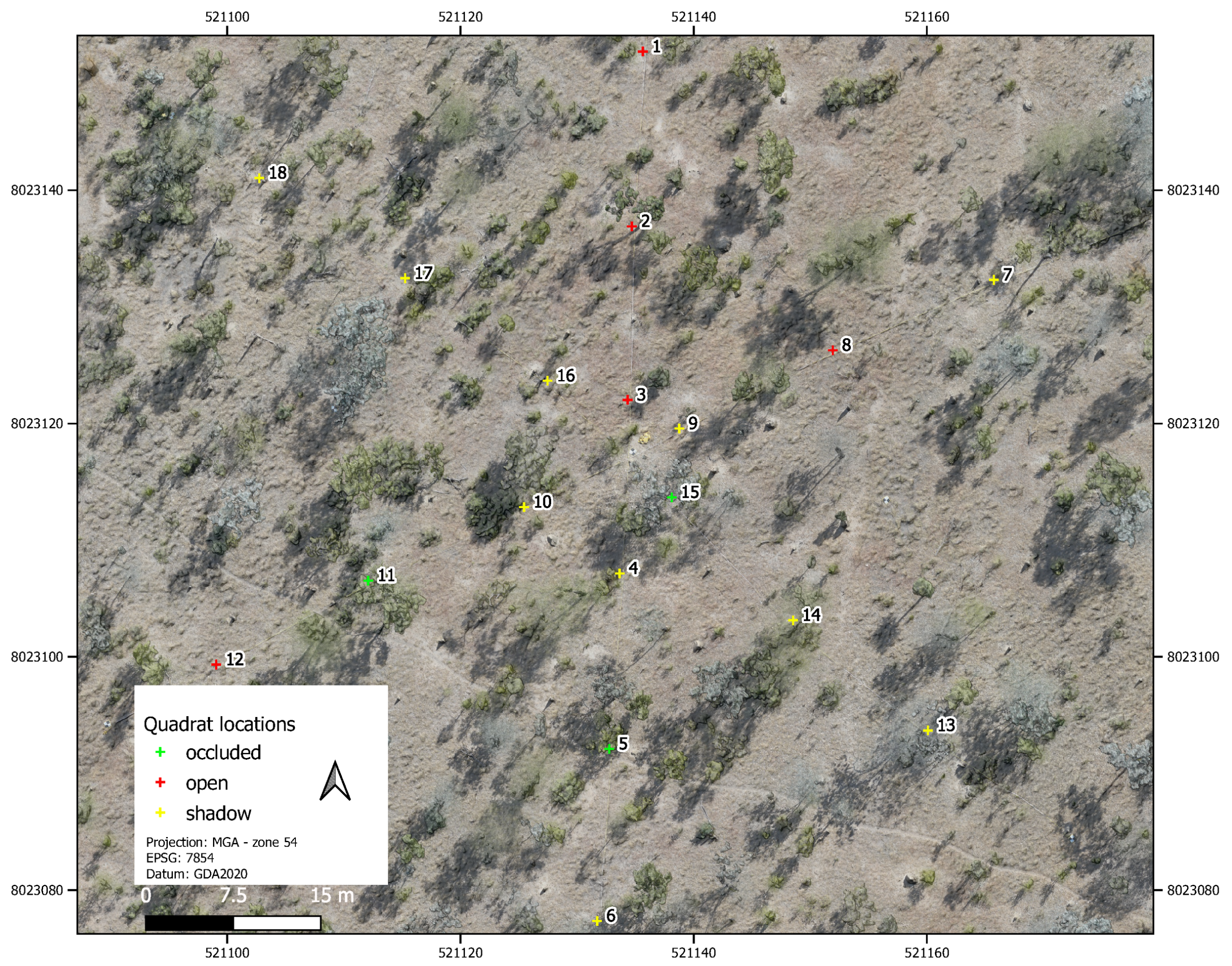
Figure 6.
Modelled TSDM yields for both modelling procedures at an independent grassland field site. Photograph (a) is first an example of the field sites pasture from its centre point, next map (b) illustrates the orthomosaic image of the field site and finally maps (c,d) illustrate the automatic ML and robust regression models of TSDM t ha−1 applied to the PHUAV modelled surface. Individual field sampled quadrats are further illustrated as red crosses across both maps (b,c) along with their field measured TSDM t ha−1.

Figure 7.
Robust regression and auto ML model results of pasture yield predictions for both the grassland and woodland categories. Auto ML regression model of the grassland (a) and woodland (b) categories, robust regression model of the grassland (c) and woodland (d) category and auto ML (e) and robust (f) regression modelling accuracy assessment results.

Figure 8.
Correlograms of both acid detergent fibre (a) and crude protein (b) with; 1. Original SRuav spectra, 2. Normalised SRuav and 3. the first derivative of the normalised SRuav spectra.
Figure 8.
Correlograms of both acid detergent fibre (a) and crude protein (b) with; 1. Original SRuav spectra, 2. Normalised SRuav and 3. the first derivative of the normalised SRuav spectra.

Figure 9.
Examples of robust regression modelling of acid detergent fibre (a) and crude protein (b) for an area of Mitchell grassland. The top map of each is a reference true colour orthomosaic image for context.
Figure 9.
Examples of robust regression modelling of acid detergent fibre (a) and crude protein (b) for an area of Mitchell grassland. The top map of each is a reference true colour orthomosaic image for context.


Table 1.
Field site characteristics.
| Woodlands | |
|---|---|
| Subcategories | Savanna (SW) & Subtropical woodlands (STW) |
| Common pasture species | Heteropogen sp., Bothriochloa sp., Eragrostis sp., Aristida sp., Chloris and Chrysopogon sp’s. |
| Associated vegetation | Eucalyptus melanophloia, E. crebra, E. maculata & E. teticornis |
| Soil types | Sandy loam to clay loam |
| No. of field sites | 9 |
| Grasslands | |
| Subcategories | Mitchell (MG) & Arid (AG) Grasslands |
| Common pasture species | Astebla sp. & Iseilema sp. (MG) & Enneapogon sp., Aristida sp. & Cenchrus sp. (AG) grass species |
| Associated vegetation | Various forbs and ephemeral grasses (MG) & numerous Acacia sps. most commonly A.aneura |
| Soil types | Dark cracking clay (MG) to sandy red earths (AG) |
| No. of field sites | 10 |
| Sampling campaigns | |
| Campaign 1 | 13, 16, 20, 22 March 2019 (4 sites) |
| Campaign 2 | 20, 25, 26 May 2019 (3 sites) |
| Campaign 3 | 20 June 2019 (1 site) |
| Campaign 4 | 6 August 2019 (1 site) |
| Campaign 5 | 14, 16 October 2019 (2 sites) |
| Campaign 6 | 25, 26 February 2020 & 6, 7, 12, 13, 16, 17 March 2020 (8 sites) |
Table 2.
UAV flight mission parameters.
| Equipment | |
|---|---|
| Aircraft | DJI M600ProTM |
| Gimbal | DJI Ronin-MXTM |
| Photogrammetry | |
| Camera | Sony Alpha 7R IITM |
| Trigger | intelliGTM wifi sync trigger |
| Lens | 24 mm; aperture priority |
| Sensor | 42 mpx; 35 mm full frame; RGB |
| Image format | JPEG file format; 15 MB per image; bit depth RGB (14) |
| Flying height | ∼50 m |
| Image size | 9-10 mm ground sampling; 75 × 50 m footprints |
| Ground speed | 1.5–2m/s |
| Image count | ∼270 per site at nadir |
| Image forward & side overlap | 85% |
| Flight time | 20–30 min |
| Flight pattern | Grid in north/south alignment; stop and turn at ends |
| Hyperspectral | |
| Sensor | Corning microHSI 410 SHARKTM |
| Trigger | Bounding area box |
| Pixel size | 9–10 mm ground sampling; 682 × 40000 pixel array |
| Swath width | 25.49 m |
| Flying height | ∼50 m |
| Oversampling | 1.0 |
| Spectral range | 400 to 1000 nm +/− 1% |
| Spectral bin size | 4 nm; 150 bands |
| Image format | 682 × 40,000 pixels; 15 GB; envi HSI image format |
| Frame rate | 160 Hz |
| Average exposure | 6000 |
| Lens | 16 mm; f-stop 1.4; zoom ∞ |
| Ground speed | 5.86 m/s |
| Flight time | 10–20 min |
| Flight pattern | Area scan in east/west alignment; 5 m end lead in distance & 5 m side overlap |
Table 3.
Photogrammetry SfM & Hyperspectral imagery processing parameters.
| Pix4D SfM photogrammetry | |
|---|---|
| Keypoints image scale | Full |
| Point cloud densification | Original image size |
| Minimum no. of matches | 3 |
| Point density | Optimal |
| Resolution | 1 × GSD |
| DSM filters | Noise filtering; sharp surface smoothing |
| Hyperspectral Ortho-rectification | |
| PARGE raw scan import | Conversion from BIL to BSQ |
| Raw navigation file | Non-DGPS GNSS L1 band receiver; Coordinate system: geographic; datum: WGS84 |
| IGM cube processing | Resampling method: Fast nearest neighbour; Exclusion/fill pixel distance: 1 pixel |
| Processing resources | |
| Desktop computing details | 128 GB RAM; 64 CPU threads; 1 × GeoForce RTX 2080 Ti GPU; 1TB M.2 SSD |
Table 4.
TPOT parameters.
| Parameter | |
|---|---|
| Generations | 1000 |
| No. of jobs | 5 |
| Population size | 100 |
| Random state | 42 |
| Config dictionary | default (all regression models) |
Table 5.
Results of Propeller AeroPointTM GCP comparison with terrestrial based survey (m).
| GCP | x1 | y1 | z1 | x2 | y2 | z2 | x3 | y3 | z3 |
|---|---|---|---|---|---|---|---|---|---|
| 1 | 456243.400 | 6974635.912 | 88.162 | 456243.445 | 6974635.937 | 88.137 | −0.044 | −0.024 | 0.025 |
| 2 | 456237.163 | 6974586.501 | 91.709 | 456237.187 | 6974586.475 | 91.672 | −0.023 | 0.026 | 0.037 |
| 3 | 456194.435 | 6974644.939 | 85.752 | 456194.468 | 6974644.965 | 85.753 | −0.032 | −0.025 | −0.001 |
| 4 | 456249.303 | 6974685.550 | 85.853 | 456249.312 | 6974685.553 | 85.915 | −0.008 | −0.002 | −0.062 |
| 5 | 456280.424 | 6974602.521 | 90.421 | 456280.444 | 6974602.505 | 90.477 | −0.019 | 0.016 | −0.056 |
| 6 | 456206.564 | 6974669.454 | 85.191 | 456206.622 | 6974669.448 | 85.242 | −0.057 | 0.006 | −0.051 |
| 7 | 456292.393 | 6974626.093 | 89.108 | 456292.419 | 6974626.051 | 89.16 | −0.025 | 0.042 | −0.052 |
| 8 | 456197.051 | 6974617.439 | 87.549 | 456197.095 | 6974617.413 | 87.629 | −0.043 | 0.026 | −0.08 |
| Average | - | - | — | - | - | — | −0.032 | 0.007 | −0.03 |
xyz1 = GCP coordinates & elevation. xyz2 = Survey coordinates & elevation. xyz3 = Differences. Coordinate projection: Map Grid of Australia zone 56. Datum: GDA2020.
Table 6.
Best linear regression models of both acid detergent fibre and crude protein for each spectral feature and data transformation including the raw spectral reflectance.
Table 6.
Best linear regression models of both acid detergent fibre and crude protein for each spectral feature and data transformation including the raw spectral reflectance.
| Nutrient Quality Measure | Spectral Feature | Transformation | B1 | B2 | r2 |
|---|---|---|---|---|---|
| ADF | Single-band | Original | 667.82 nm | - | 0.648 |
| Normalised | 651.81 nm | - | 0.896 | ||
| First derivative | 543.78 nm | - | 0.466 | ||
| CP | Single-band | Original | 759.85 nm | - | 0.160 |
| Normalised | 759.85 nm | - | 0.502 | ||
| First derivative | 551.78 nm | - | 0.287 | ||
| ADF | Simple ratio | Original | 655.82 nm | 919.91 nm | 0.897 |
| Normalised | 655.82 nm | 919.91 nm | 0.897 | ||
| First derivative | 667.82 nm | 475.75 nm | 0.794 | ||
| CP | Simple ratio | Original | 947.92 nm | 939.92 nm | 0.745 |
| Normalised | 947.92 nm | 939.92 nm | 0.745 | ||
| First derivative | 947.92 nm | 939.92 nm | 0.625 | ||
| ADF | NDSI | Original | 651.81 nm | 939.92 nm | 0.903 |
| Normalised | 651.81 nm | 939.92 nm | 0.903 | ||
| First derivative | 475.75 nm | 667.82 nm | 0.792 | ||
| CP | NDSI | Original | 939.92 nm | 947.92 nm | 0.742 |
| Normalised | 939.92 nm | 947.92 nm | 0.742 | ||
| First derivative | 939.92 nm | 947.92 nm | 0.624 |
Publisher’s Note: MDPI stays neutral with regard to jurisdictional claims in published maps and institutional affiliations. |
© 2020 by the authors. Licensee MDPI, Basel, Switzerland. This article is an open access article distributed under the terms and conditions of the Creative Commons Attribution (CC BY) license (http://creativecommons.org/licenses/by/4.0/).
Share and Cite
MDPI and ACS Style
Barnetson, J.; Phinn, S.; Scarth, P. Estimating Plant Pasture Biomass and Quality from UAV Imaging across Queensland’s Rangelands. AgriEngineering 2020, 2, 523-543. https://0-doi-org.brum.beds.ac.uk/10.3390/agriengineering2040035
AMA Style
Barnetson J, Phinn S, Scarth P. Estimating Plant Pasture Biomass and Quality from UAV Imaging across Queensland’s Rangelands. AgriEngineering. 2020; 2(4):523-543. https://0-doi-org.brum.beds.ac.uk/10.3390/agriengineering2040035
Chicago/Turabian StyleBarnetson, Jason, Stuart Phinn, and Peter Scarth. 2020. "Estimating Plant Pasture Biomass and Quality from UAV Imaging across Queensland’s Rangelands" AgriEngineering 2, no. 4: 523-543. https://0-doi-org.brum.beds.ac.uk/10.3390/agriengineering2040035