Mapping Wheat Dry Matter and Nitrogen Content Dynamics and Estimation of Wheat Yield Using UAV Multispectral Imagery Machine Learning and a Variety-Based Approach: Case Study of Morocco

Abstract

Our work aims to monitor wheat crop using a variety-based approach by taking into consideration four different phenological stages of wheat crop development. In addition to highlighting the contribution of Red-Edge vegetation indices in mapping wheat dry matter and nitrogen content dynamics, as well as using Random Forest regressor in the estimation of wheat yield, dry matter and nitrogen uptake relying on UAV (Unmanned Aerial Vehicle) multispectral imagery. The study was conducted on an experimental platform with 12 wheat varieties located in Sidi Slimane (Morocco). Several flight missions were conducted using eBee UAV with MultiSpec4C camera according to phenological growth stages of wheat. The proposed methodology is subdivided into two approaches, the first aims to find the most suitable vegetation index for wheat’s biophysical parameters estimation and the second to establish a global model regardless of the varieties to estimate the biophysical parameters of wheat: Dry matter and nitrogen uptake. The two approaches were conducted according to six main steps: (1) UAV flight missions and in-situ data acquisition during four phenological stages of wheat development, (2) Processing of UAV multispectral images which enabled us to elaborate the vegetation indices maps (RTVI, MTVI2, NDVI, NDRE, GNDVI, GNDRE, SR-RE et SR-NIR), (3) Automatic extraction of plots by Object-based image analysis approach and creating a spatial database combining the spectral information and wheat’s biophysical parameters, (4) Monitoring wheat growth by generating dry biomass and wheat’s nitrogen uptake model using exponential, polynomial and linear regression for each variety this step resumes the varietal approach, (5) Engendering a global model employing both linear regression and Random Forest technique, (6) Wheat yield estimation. The proposed method has allowed to predict from 1 up to 21% difference between actual and estimated yield when using both RTVI index and Random Forest technique as well as mapping wheat’s dry biomass and nitrogen uptake along with the nitrogen nutrition index (NNI) and therefore facilitate a careful monitoring of the health and the growth of wheat crop. Nevertheless, some wheat varieties have shown a significant difference in yield between 2.6 and 3.3 t/ha.

1. Introduction

Precision agriculture has demonstrated its potential by englobing advanced technologies to ensure efficiency gains and to alleviate food security allowing the implementation of modern management and decision tools [1]. As an ever-evolving discipline, precision agriculture has proven its efficiency when it comes to overcoming the major limits of research aiming to tackle climate variations along with excessive consumption. Therefore, analysts foresee an agro-technological revolution, where precision agriculture is believed to play a key role as an innovative production system, which relies on input management in a field based on actual crop needs while optimizing deployed resources [2,3]. For this purpose, it aims to control the production chain and the factors that influence it by exploiting new technologies such as GNSS (Global Navigation Satellite System) and remote sensing to manage crops and reduce the use of fertilizers, pesticides and water [4].

A recent study by Hexa Reports suggests that precision agriculture is expected to reach 43.4 billion dollars by 2025 [5]. Hence, it is viewed as a promising field in continued expansion, including the use of the remote sensing approach, which offers a viable alternative for determining crop status due to its ability to capture large areas at the same time [6] Especially with the widespread of the use of UAV technology allowing a low-altitude remote sensing and the ability to use various sensors thermal, hyperspectral and optical [7,8]. This discipline is ubiquitous in Morocco because of its predominantly agricultural economy, where the national production of cereals is highly exposed to climate fluctuations because it is concentrated mainly in arid and semi-arid areas with limited land and water resources [9].

Wheat is one of the most highly regarded crops for national monitoring because it has been an essential food source for the population for centuries [10]. Therefore, the prediction of its yield is a necessity since it is a tool of great interest for decision-making and the basis of measured planning [11]. Indeed, in order to ensure food security, yield prediction makes it possible to prepare for the consequences of an agricultural shortage, by reducing vulnerability to climatic hazards and to plan in advance aid to farmers and cereal imports. In the case of agricultural insurance, yield estimation quantifies the impacts of droughts when they occur to properly determine compensation. It also allows producers who commit to export their crops to plan their actions and decision based on the results of the prediction [12]. Thus, several studies have been conducted to predict wheat yield. We specify the study of Hassan et al. in 2018 [13], which was held in China specifically in Beijing and its objective is to estimate the agricultural yield of wheat for 32 varieties, six flight missions that correspond to the following phenological stages: heading, flowering, seed development (Beginning of the stadium milky, soft pasty stage and hard pasty) were made with flight heights between 30 m and 40 m in order to reach spatial resolutions of 2.5 cm to 2.8 cm by the Sequoia camera. Moreover, the data acquisition was conducted over two phases. Firstly, the extraction of the 9 m² plots allowed obtaining the following in-situ data: Number of grains per ear and number of ears for each plot. Secondly, the use of Sequoia multispectral camera and Pix4D Mapper for data post-processing allowed the use of the following vegetation indices: GNDVI, SR-NIR, RECI and NDRE. A correlation between the vegetation indices and the in-situ data using R package for linear regression gave a coefficient of determination R² greater than 0.80 in the soft pasty stage between the different vegetation indices and the in-situ collected data [10]. Similarly, and using the K-means model, Guan et al. in 2019 [14] has explained the use of unmanned aerial vehicle (UAV) and multispectral imagery in the agricultural field. Their work was to calculate the agricultural yield of wheat and rice. For wheat cultivation UAV flight missions have been programmed with a flight height ranging from 30 m to 100 m and using the Parrot Sequoia camera. 24 plots were collected between flowering and maturity phenological stages and having an area of 8 m × 14 m. The NDVI (Normalized Difference Vegetation Index) is the only vegetation index used, which resulted in a coefficient of determination of 0.81 with wheat yield during the grain development stage [13].

Throughout this study we aim to:

• Monitor wheat crop and estimate its yield using UAV technology multispectral imagery.
• Evaluate the use of the Red-Edge band in agricultural remote sensing applications.
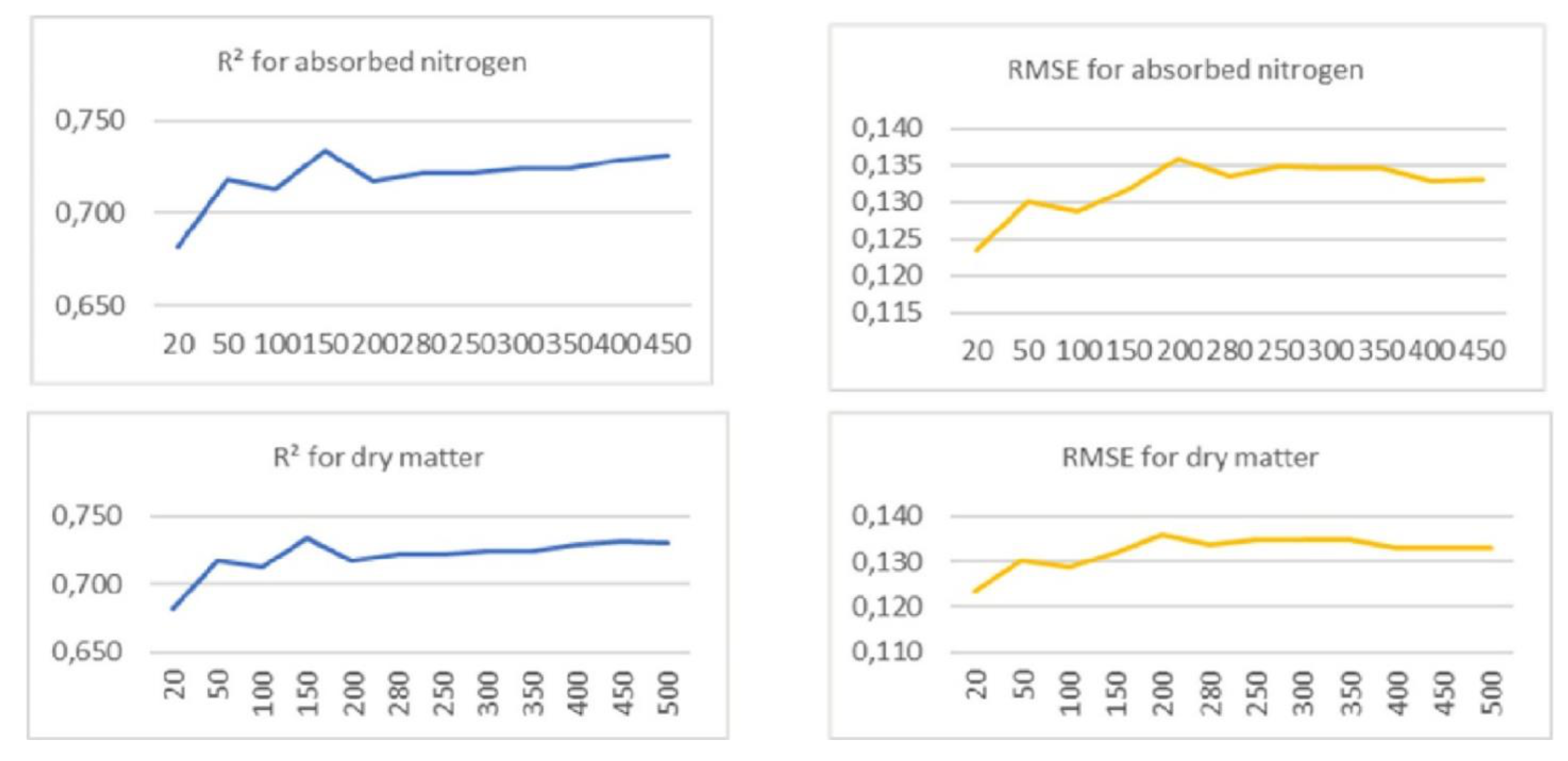
• Use of regression functions and Random Forest as a machine learning technique for prediction purposes in agriculture.
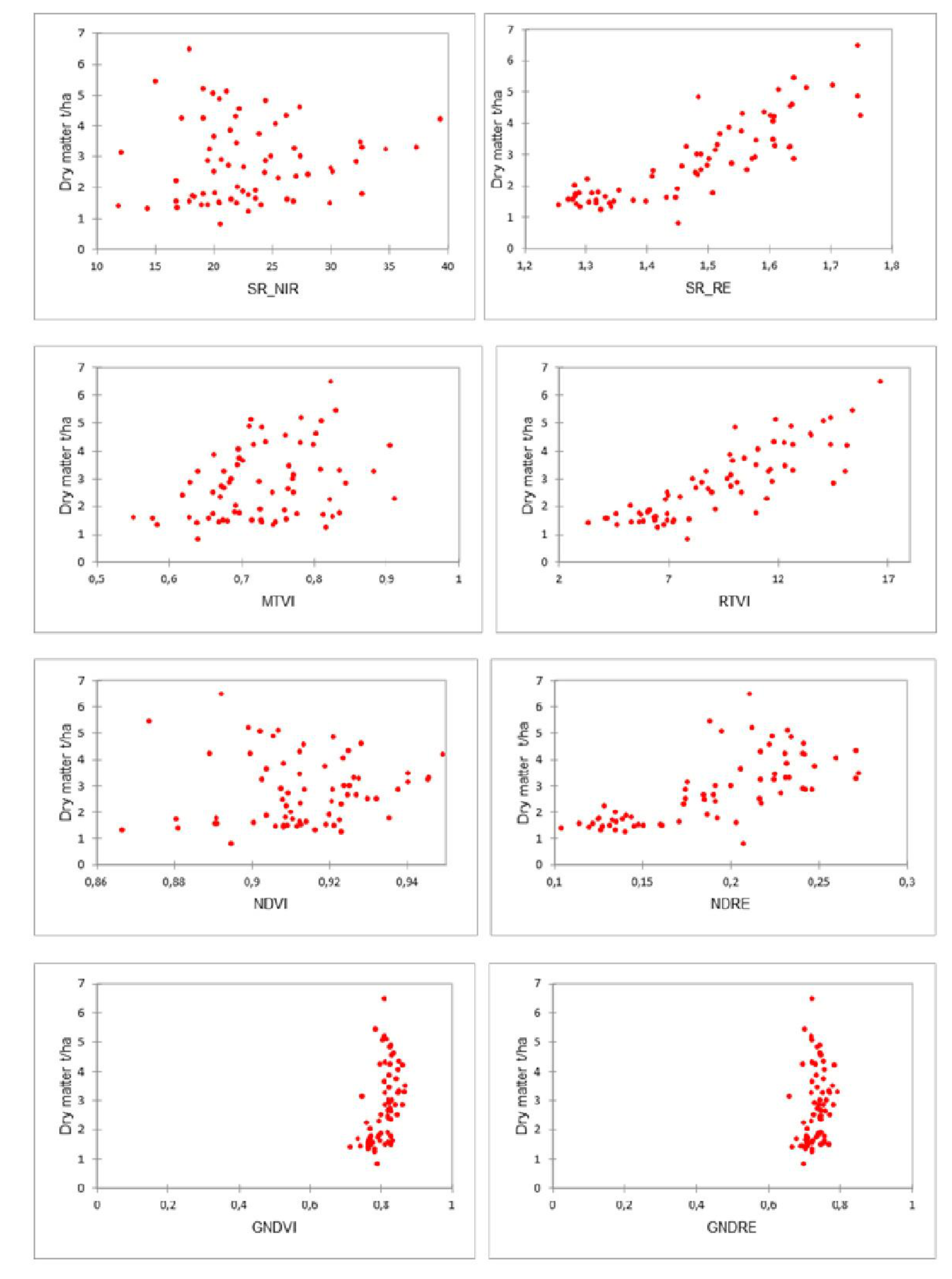
• Elucidate the ability of different vegetation indices to estimate the biophysical parameters of wheat crop, namely dry matter and nitrogen uptake considering wheat’s phenotypical diversity and phenological stages.

In the following paper, we will discuss three main sections: the first one enumerates the material and the methods used, the second is a presentation of the obtained results followed by a discussion. The last section is an overall conclusion and recommendations allowing a quick overview and confrontation of the present work with those to come.

2. Materials and Methods

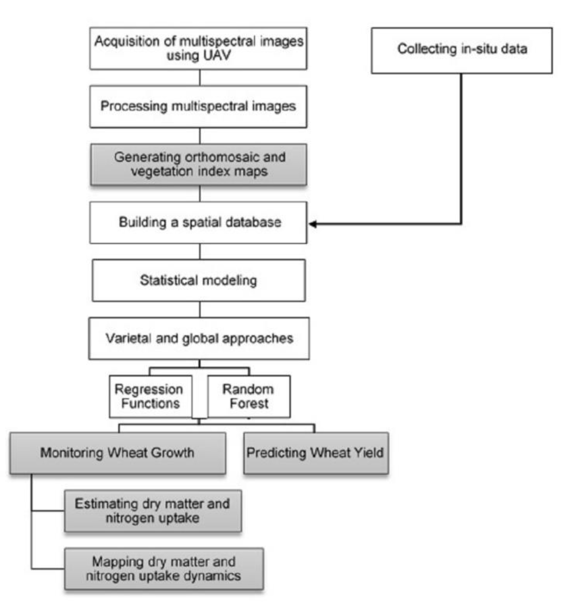
2.1. General Methodology

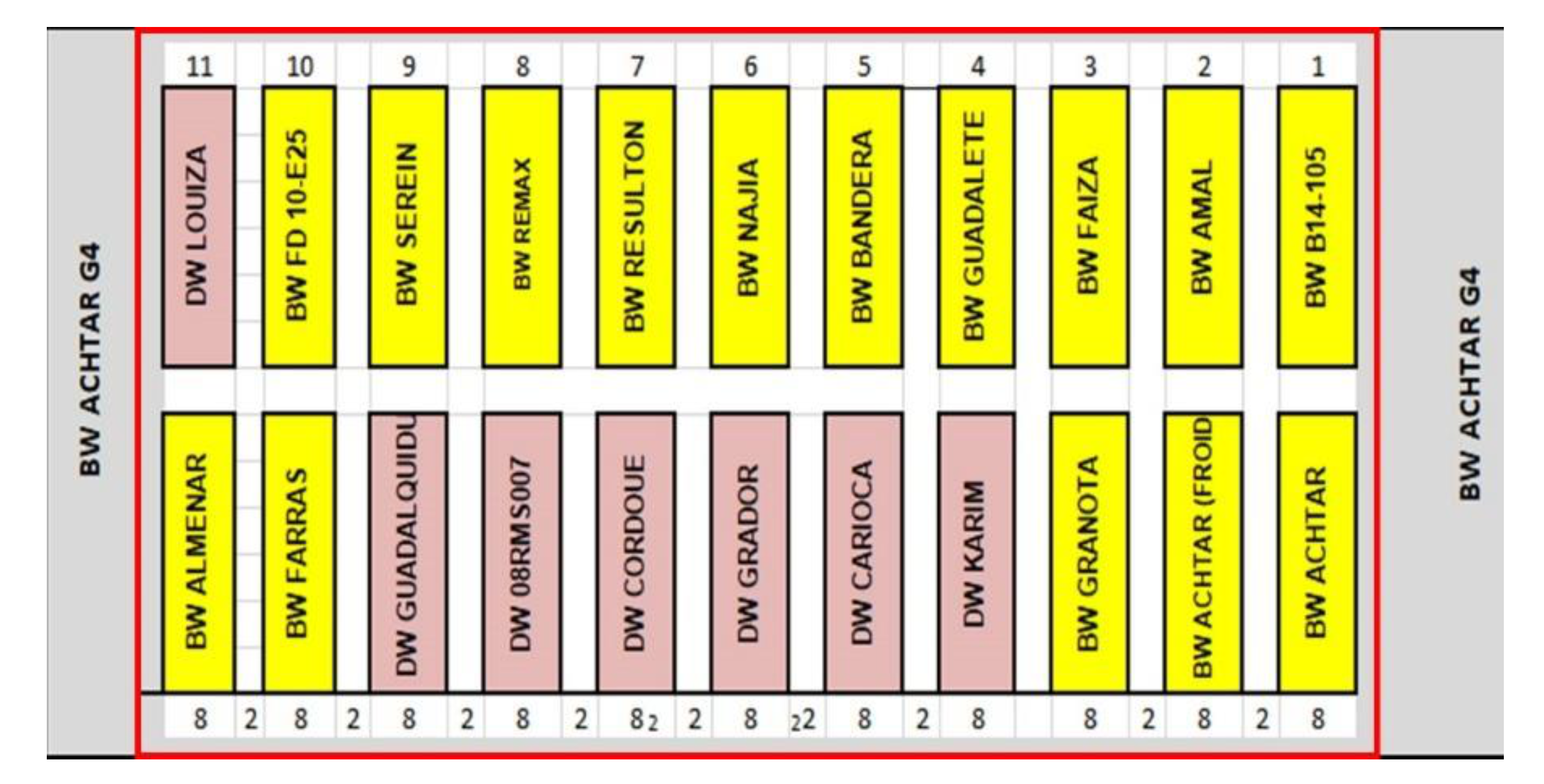
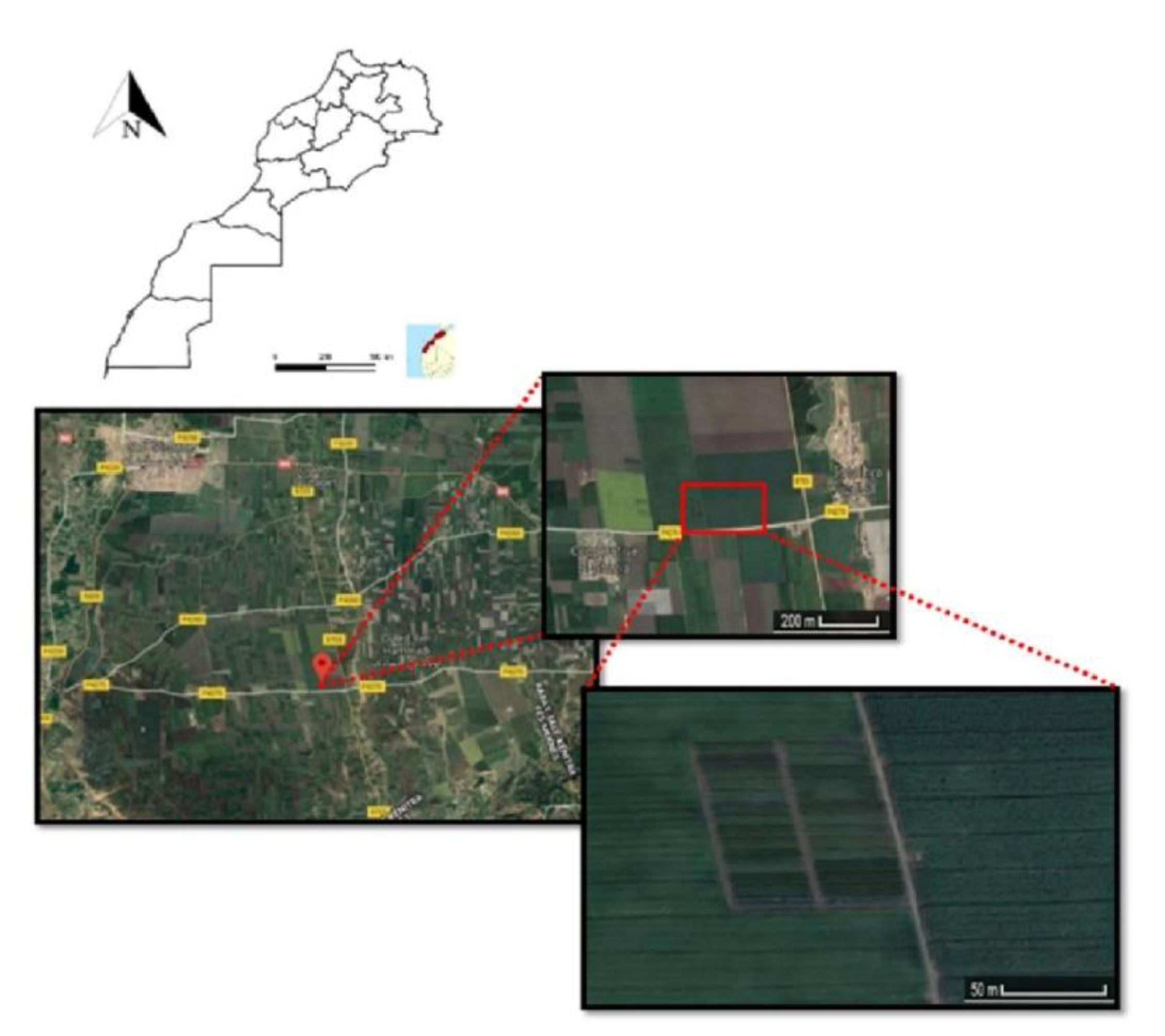
Having a multispectral camera as a payload, the use of UAV allowed the execution of several flight missions during various stages of wheat development, namely the end of tillering, two nodes, the flag leaf fully unrolled and during the ripening stage before and after extraction of the plots. The images resulting from the executed missions were post-processed and hence permitted the generation of the following outputs: orthomosaic and vegetation index maps: NDVI, NDRE, GNDVI, GNDRE, SR-RE, SR-NIR, RTVI and MTVI2. By using both UAV’s multispectral imagery and in-situ data, a database containing both vegetation index values and the biophysical parameters of wheat crop, dry matter and nitrogen uptake was created.

The approach adopted in this study (Figure 1) is primarily to analyze the response of each vegetation index to each wheat variety in order to decide on the hypothesis of variation of vegetation indices by genotype of wheat and according to the biophysical characteristics of each variety. After that, a general approach that consists of establishing a model utilizing firstly the Random Forest technique and secondly a linear regression. For UAV’s imagery we have used World Geodetic System 1984 or WGS84 before generating the UAV’s products. Therefore, during this whole study we have used Merchich North Morocco’s coordinate system for georeferenced orthomosaics, reflectance and vegetation indices maps.

2.2. Study Area

This study took place in Morocco at the experimental platform of the agricultural domain HAMMA located in the province of Sidi Slimane (Figure 2). The experimental platform used in our study is exploited essentially for durum and bread wheat crop cultivation. It is composed of 28 micro-platforms of 300 m² each with different varieties. The sowing date is 06 of December 2018. The general disposition of microplatforms upon the experimental platform is presented in Figure 3 where DW stands for durum wheat and BW stands for bread wheat.

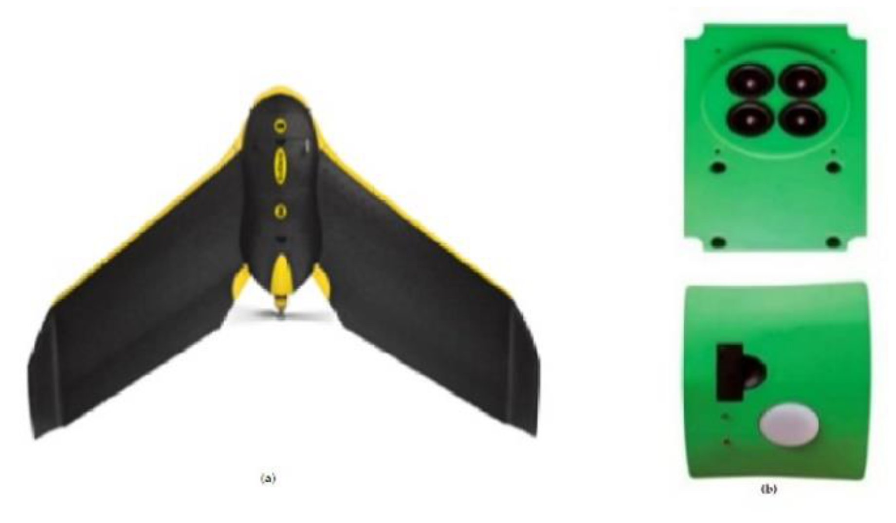
2.3. UAV and In-Situ Data Acquisition

2.3.1. Acquisition of UAV’s Multispectral Imagery

The used UAV platform was eBee Classic with MultiSPEC 4C camera as a payload (Figure 4).

Table 1. UAV and camera specifications.

UAV Specifications			Camera Specifications
UAV type	Fixed-wing	Sensor type	4 × 1/3″ CMOS
Weight (including battery and payload)	690 g	Acquisition bands	Green (550 nm)—Red (660 nm)—Red-Edge (735 nm)—NIR (790 nm)
Radio link range	3 km	Storage	SD card
Piloting	Automatic	Focal length	4 mm
Speed	40–90 km/h	F-number	f/1.8
Wind resistance	Up to 12 m/s	Shutter type	Global shutter
Nominal maximal flight time	50 min	Degrees of freedom	Nadiral acquisition only
Landing	Linear (precision of 5 m)	Weight	160 g
Absolute horizontal/vertical precision (using GCP)	Up to 3 cm/5 cm	Output image	4 Images in tif format with raw 10 bits
Absolute horizontal/vertical precision (without using GCP)	1–5 m	Ground/spatial resolutions	5–30 cm

presents some main characteristics of the used UAV platform and the multispectral camera. Seven flight missions were executed at different dates during different stages of wheat growth. At each phenological stage, two flights before and after the sampling are conducted. The objective of having two flights is to be able to find the location of the experimental plots after postprocessing the images. An individual final mission was done during the maturity stage. However, planning a UAV flight mission is a crucial step that conditions the spatial and spectral resolution of the resulting images [14]. And knowing that fixed-wing UAVs are more susceptible to external disturbances, we have taken into account the following parameters due to their importance in precision agriculture purposes: Flight altitude, wind speed, longitudinal and lateral overlaps as well as safe take-off and landing sites using the same ROI (Region of Interest) polygon of the experimental platform [15,16].

The characteristics of each mission by phenological stage are presented in the

Table 2. Characteristics of UAV’s flight missions during different stages of wheat growth.

	Flight 1	Flight 2	Flight 3	Flight 4	Flight 5	Flight 6	Flight 7
Duration	10 min	10 min	10 min	10 min	10 min	10 min	10 min
Flight altitude	60 m	60 m	60 m	60 m	60 m	60 m	60 m
GSD	6 cm	6 cm	6 cm	6 cm	6 cm	6 cm	6 cm
Lateral overlap	70%	70%	70%	70%	70%	70%	70%
Longitudinal overlap	80%	80%	80%	80%	80%	80%	80%
Covered area	6 ha	6 ha	6 ha	6 ha	6 ha	6 ha	6 ha
Mission date	12 February 2019		22 February 2019		14 March 2019		15 May 2019
Phenological stage	End of tillering		Two nodes		Flag leaf fully unrolled		Ripening

.

Before executing the flight missions using the MultiSPEC 4C camera, radiometric calibration images must be taken. This calibration is performed to obtain reflectance measurements from the acquired images. It is performed using a calibration target provided by the manufacturer. To succeed the calibration process, the lighting conditions of the sensor of multiSPEC 4C camera and the calibration target must be identical to the lighting conditions encountered by the eBee during its mission (Figure 5). Thus, the target must be exposed to the sky and clear of shadows during the calibration procedure. The UAV must be placed above the target, it must be horizontal, with a minimum distance of 50 cm and maximum of 1 m (Technical Guide MultiSPEC 4C). Once placed, the camera automatically takes several calibration images, with a pause of about 3 s between each image.

2.3.2. Collecting In-Situ Data

During plant growth, field samples are taken at the end of tillering stage (BBCH (Biologische Bundesanstalt bunderssortenamt and CHemical industry) 29–30), two nodes (BBCH 32) and flag leaf fully unrolled (BBCH 39). These samples count three plots of 0.5 m × 0.5 m each, chosen so that they can reveal the state of the whole microplatform. Measurements are made on each plot, which enables quantitative and qualitative data to be collected on the state and development of the crop. The objective of this step is to quantify the biophysical parameters and nutrient uptake of wheat for each variety. It is thus enrolled on two phases:

• Field phase:

The data collected directly from the field, at the level of each plot and at each stage are: Length of the stem, presence of pests, weeds and diseases, state of the plant and weight of the sample.

• Laboratory phase:

Samples of 50 to 100 plants are collected and sent to the laboratory to extract the following results: Fresh matter, dry matter and total nitrogen content. The quantity of fresh and dry matter is estimated by measuring the weight of the sample of the collected plants with a balance (fresh weight) then dried for 24 to 48 h at 80 °C (constant weight), cooled and weighed again (weight dry). For the nitrogen content Dumas combustion method was used [17].

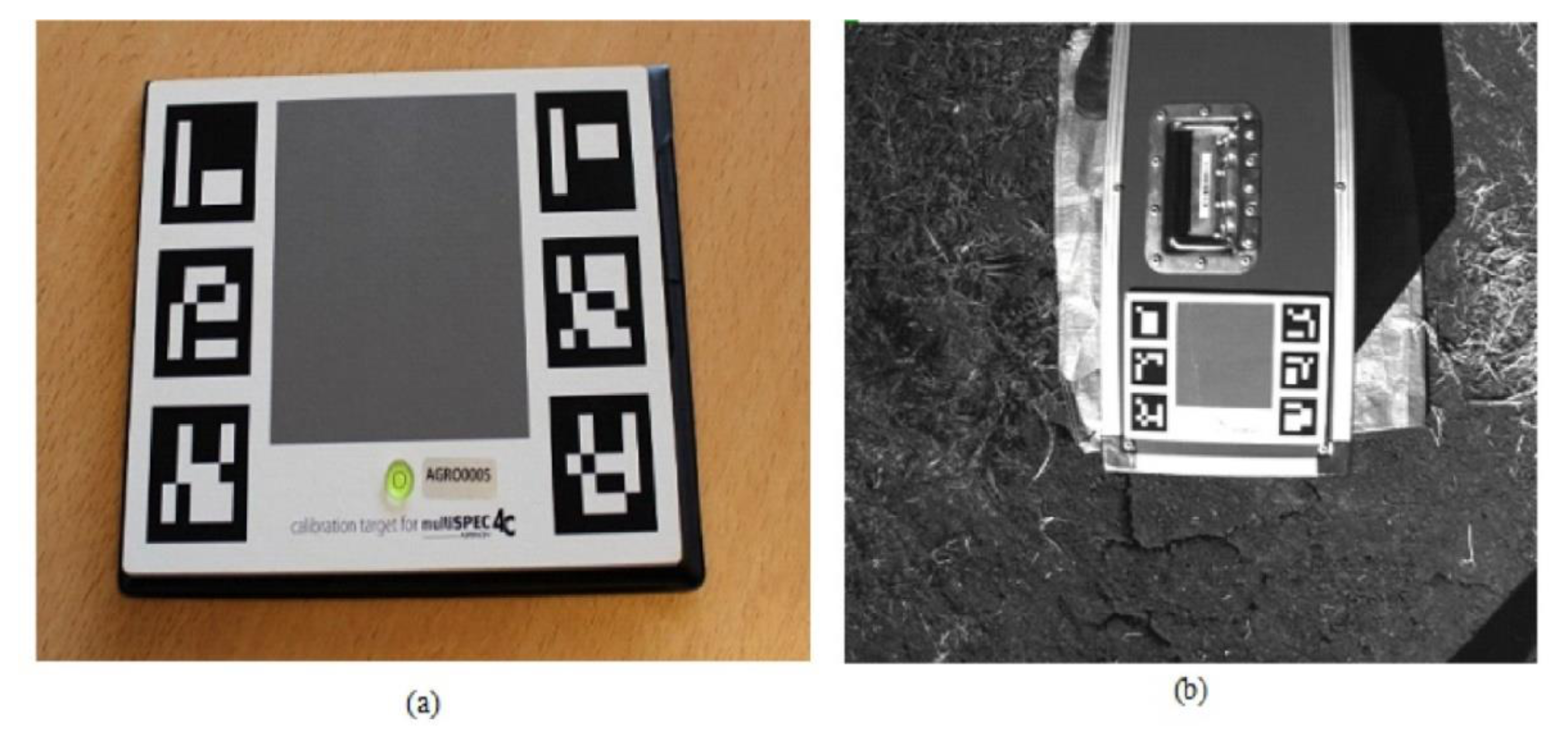
2.4. Multispectral UAV Images Processing

First, the acquired images were preprocessed and geolocated using the trajectory data contained in the EXIF and Log files. The radiometric calibration of the images was also performed while automatically selecting the coefficients resulting from the calibration targets (Airinov Aircalib used in our case is included among the targets detected automatically by Pix4D) performed using the calibration images acquired before each flight and for each multispectral band [18]. The use of a radiometric calibration target makes it possible to calibrate and correct the radiance values of the pixels according to the values given by the calibration target by taking into account the lighting conditions on the date, at the same time and location of the image capture [19].

The processing of acquired UAV images was conducted for each flight mission. We used Pix4D [20] solution for this purpose. The workflow consists of three main steps: Initial processing, generating dense point clouds and generating digital surface models (DSM), orthomosaics and reflectance maps [21]. During the initial processing, the position of the matching points is calculated. These points are used to consolidate the correspondence between images. Subsequently, an AAT (Automatic Aerial Triangulation) and a bundle block adjustment (BBA) are executed which allow the calculation of the 3D position of the camera at each capture as well as the coordinates of the matching points. Finally, automatic matching points are created and thus constituting the basis for the next processing steps (Pix4D support). The next step is the generation of a dense point cloud where additional tie points are created based on the automatic connection points that result in a dense point cloud and a 3D textured mesh which can be created using the dense point cloud. The final step aims to create a digital surface model (DSM) that allows the generation of orthomosaic and reflectance maps.

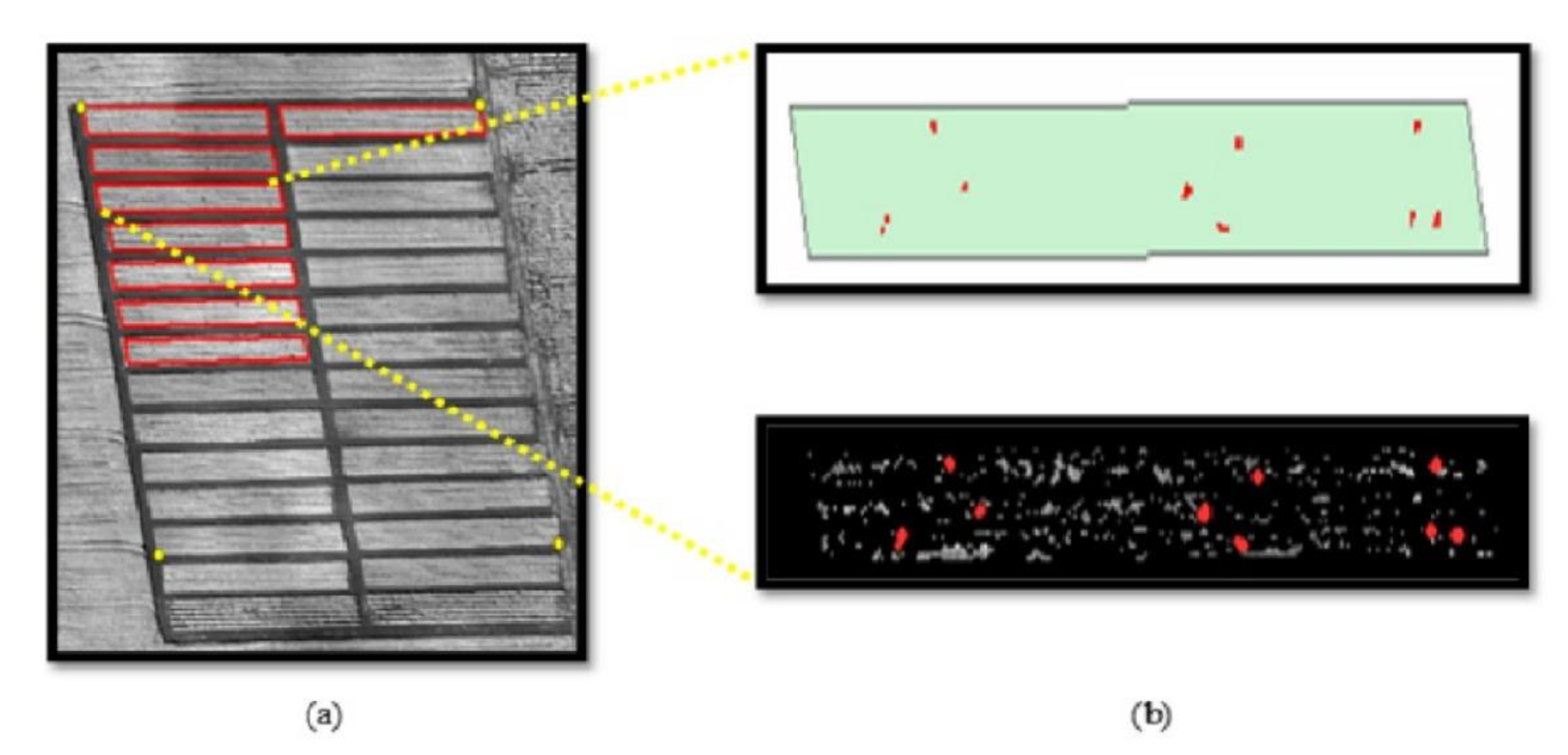
2.5. Automatic Extraction of Plots

The objective of this step is to extract the field plots during each phenological stage from the corresponding UAV imagery (Figure 6). First, the orthomosaics of each band (NIR, Red, Green and Red-Edge) were readjusted before and after sampling using calibration points. In order to eliminate soil surrounding the experimental plots, one mask of each microplatform was then created per multispectral band for the flag leaf fully unrolled stage orthomosaic. And in order to automatically extract the experimental plots, we used an object-based image analysis approach (eCognition [22]). We first conducted a chessboard segmentation to create objects which size is equal to that of pixels, followed by a spectral difference segmentation based on a merging algorithm in which neighboring objects where the spectral average is below a given threshold (maximum spectrum difference in our case 13) will be merged to produce the final objects. To use the latter algorithm, a prior segmentation was necessary [23]. After which multiresolution segmentation was performed having as parameters a scale of 100, 0.9 for shape and 0.9 for compactness. We finally performed a classification step enabling the extraction of the plots’ positions and their reflectance values.

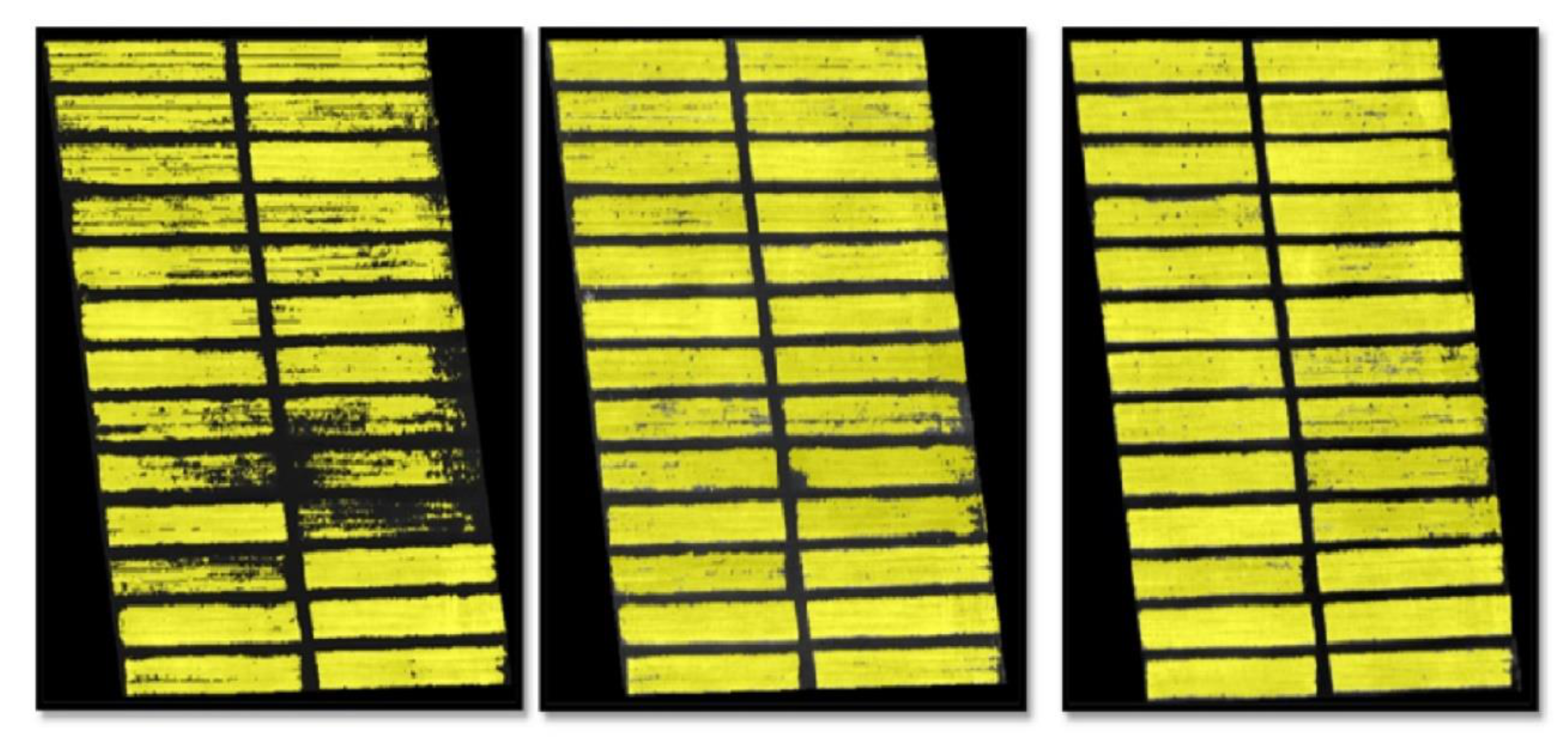
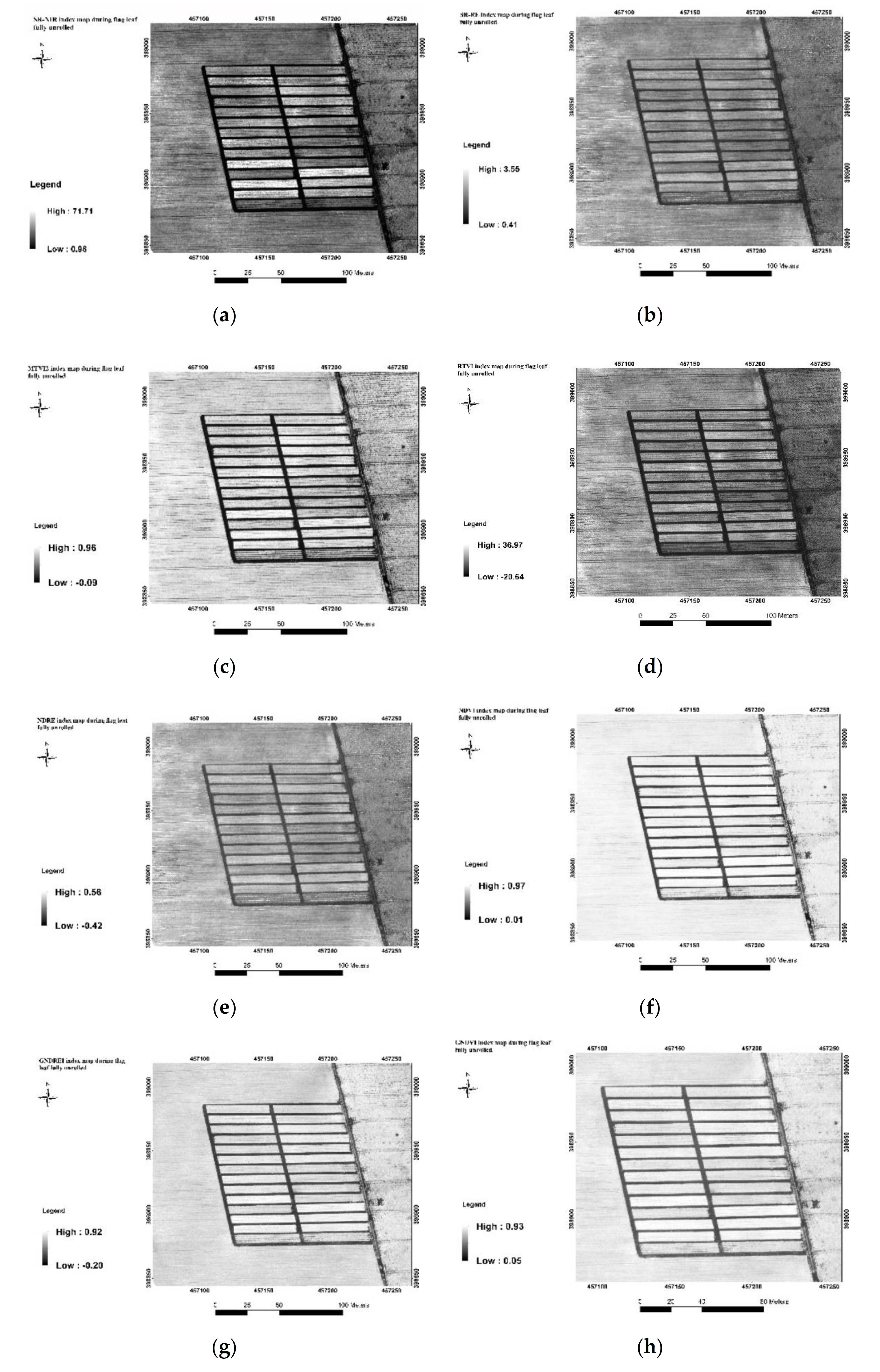
2.6. Generation of Vegetation Index Maps

We then calculated the vegetation indices maps in which the value of each pixel is calculated using a formula combining different bands of reflectance maps. Throughout this study, we used eight vegetation indices. We chose indices that used different spectral bands to evaluate the effect of integrating the Red-Edge band. Other criteria upon which we built our choice is the nature of the combination and the number of bands used by the index.

Table 3. Vegetation indices formulas and references.

Index	Formula	Reference
Simple Ratio	${\mathrm{R}}_{\mathrm{NIR}}$$/{\mathrm{R}}_{\mathrm{Red}}$	Birth et al. (1968)
Simple Ratio Red Edge	${\mathrm{R}}_{\mathrm{NIR}}$$/{\mathrm{R}}_{\mathrm{RedEdge}}$	Zacro-Teiada et al. (1999)
NDVI	$({\mathrm{R}}_{\mathrm{NIR}}$$-$${\mathrm{R}}_{\mathrm{Red}})/({\mathrm{R}}_{\mathrm{NIR}}$$+{\mathrm{R}}_{\mathrm{Red}})$	Rouse et al. (1974)
NDRE	$({\mathrm{R}}_{\mathrm{NIR}}-{\mathrm{R}}_{\mathrm{RedEdge}})/({\mathrm{R}}_{\mathrm{NIR}}$$+{\mathrm{R}}_{\mathrm{RedEdge}})$	Fitzgerald et al. (2010)
GNDVI	$({\mathrm{R}}_{\mathrm{NIR}}$$-$${\mathrm{R}}_{\mathrm{Green}})/({\mathrm{R}}_{\mathrm{NIR}}$$+{\mathrm{R}}_{\mathrm{Green}})$	Gitelson et al. (1996)
GNDRE	$({\mathrm{R}}_{\mathrm{RedEdge}}$$-$${\mathrm{R}}_{\mathrm{Green}})/({\mathrm{R}}_{\mathrm{RedEdge}}$$+{\mathrm{R}}_{\mathrm{Green}})$	Cao et al. (2013)
MTVI2	$\frac{1.5\times \left(1.2\times \left({\mathrm{R}}_{\mathrm{NIR}}-{\mathrm{R}}_{\mathrm{Green}}\right)-2.5\times \left({\mathrm{R}}_{\mathrm{Red}}-{\mathrm{R}}_{\mathrm{Green}}\right)\right)}{\sqrt{((\left(2\times {\mathrm{R}}_{\mathrm{NIR}}+1\right)^2)-(6\times {\mathrm{R}}_{\mathrm{NIR}}-5\times \sqrt{({\mathrm{R}}_{\mathrm{Red}})}-0.5))}}$	Haboudane et al. (2004)
RTVI	$100({\mathrm{R}}_{\mathrm{NIR}}$$-$${\mathrm{R}}_{\mathrm{RedEdge}})$$-10({\mathrm{R}}_{\mathrm{NIR}}$$-$${\mathrm{R}}_{\mathrm{Green}}$)	Chen et al. (2010)

presents the indices used in this study.

2.7. Building a Spatial Database for the Experimental Platform

The extraction of experimental plots during each flight allowed the attribution of in-situ data by establishing a database combining both the geographic information contained in the result of the extraction and the biophysical parameters of each plot using an attribute table. Moreover, the extraction of spectral information of each plot was performed using vegetation index maps and added to the attribute table. Similarly, extracting microplatforms was necessary so as to quantify dry biomass and nitrogen content and prevent the soil component from being considered during the modeling phase. A rule set was implemented on eCognition for each stage of wheat development and using the selected vegetation index from the varietal approach using both segmentation and classification methods. The obtained mask was subsequently exported in .tif format and then applied (Figure 7).

2.8. Monitoring Wheat Growth

Monitoring wheat growth was performed using two biophysical parameters of wheat: the nitrogen uptake and the amount of dry matter. This step consists of determining the statistical models that will allow the calculation of the two biophysical parameters of wheat from the vegetation indices mentioned previously. To do this, we adopted two approaches: Varietal approach and general approach.

2.8.1. Varietal Approach

To take into consideration the genetic difference between the different varieties of wheat, a modeling exercise was carried out for each of the eight microplatforms where the in-situ data were taken. The purpose of this approach is to evaluate the response of each vegetation index to the diversity of wheat varieties and its ability to estimate the dry matter and nitrogen uptake using the following regression models: linear regression, second order polynomial regression and exponential regression. The result of this step is the calculation of the determination parameters (R² and RMSE) of each regression model that expresses dry biomass (t/ha) and nitrogen uptake (Unit/ha) as a function of each vegetation index. This approach also allowed us to select and determine the best-suited vegetation index and the regression model to express the nitrogen uptake and the dry matter for each variety using RMSE and R² metrics.

2.8.2. General Approach

This approach consists in generalizing the statistical modeling for all the varieties of our experimental platform, in order to be able to estimate wheat yield for the all present wheat varieties given the absence of in-situ data for these microplatforms. The generalization of the model was based on the selected vegetation index using a prior varietal approach. On the first hand, the model was generalized using regression functions after which the model presenting a high value of R² and a low RMSE was maintained. On the other hand, the estimation of wheat yield and biophysical parameters for plots using the machine learning method Random Forest (RF) which is an ensemble learning method that uses multiple decision trees, with the ability to obtain a good fit and reduce noise. Where the final estimation result is obtained by voting [24]. RF was performed given its satisfactory results when used to predict biophysical parameters of different plant varieties, particularly wheat [25,26]. Random Forest was employed using Scikit-Learn library and Spyder IDE on Anaconda [27,28]. A python script was developed to model the amount of dry matter and nitrogen uptake thus estimate these parameters for each microplatform.

One of the important parameters of the RF regression is n_estimators (Number of estimators) defined as the number of trees in the random forest [29]. We conducted a set of tests to see how RF works, a sequence of numbers of the estimators has been produced from 20 up to 500. The final value of the n-estimators parameter was fixed iteratively and according to the coefficient of determination R² and RMSE (Maximize the value of R² and minimize that of the RMSE) (Figure 8). For each new choice of parameters, the value of the Random_State parameter is set to 0, which makes the output of the model replicable for the same inputs. By analyzing the obtained results, we notice that a number of estimators equal to 150 for the nitrogen uptake shows a high R² values and a low RMSE from which a stagnation of R² as well as a stationary variation of the RMSE are observed. Similarly, the R² curve peaks at the value 150 of the number of dry matter estimators, which justifies the adoption of this value for the training of the random forest regression model.

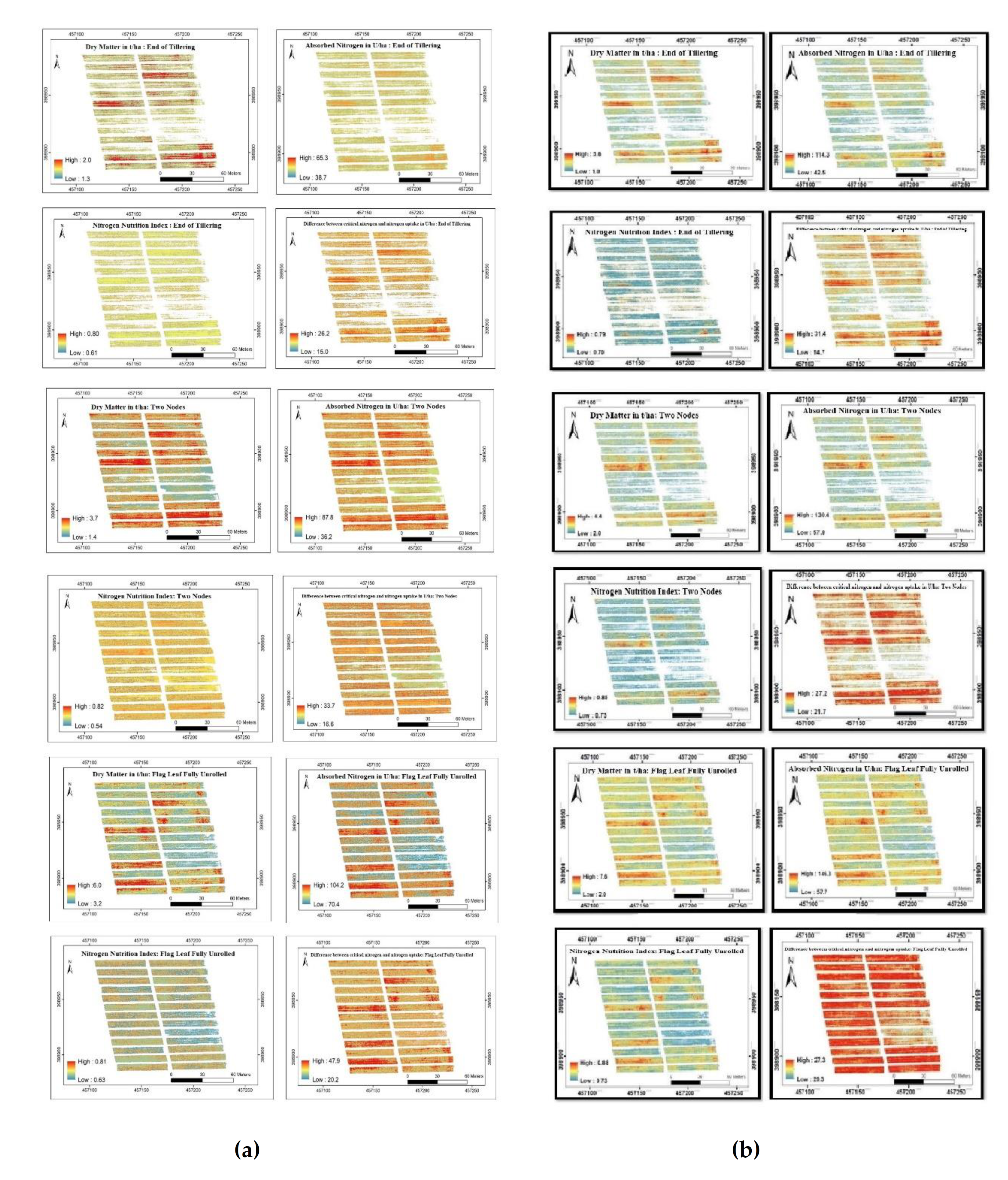
2.9. Mapping Critical Nitrogen, Dry Biomass and Nitrogen Nutrition Index

The difference between critical nitrogen and nitrogen uptake maps indicates the required nitrogen need to be added for the plant to ensure its normal development and maximize dry matter production. The values of the map of the difference between critical nitrogen and nitrogen uptake are in units of nitrogen per hectare. Whereas the model used to quantify the critical nitrogen value is the one of Justes et al. (1995) [30], which states:

$$\left\{\begin{array}{l}\mathrm{if}\mathrm{DM}>1.5\mathrm{t}/\mathrm{ha}\mathrm{then}\mathrm{N}\%=5.35{\mathrm{DM}}^{-0.442}\\ \mathrm{if}\mathrm{DM}<1.5\mathrm{t}/\mathrm{ha}\mathrm{then}\mathrm{N}\%=4.4\end{array}\right.$$

(1)

where DM is the dry matter expressed in t/ha and N (%) the total concentration of nitrogen.

For mapping the nitrogen nutrition index (NNI), we used following model [31]:

$$\mathrm{NNI}=\frac{\mathrm{N}(\%)}{{\mathrm{N}}_{\mathrm{critical}}(\%)}$$

(2)

where:

N (%): the total concentration of nitrogen

N_critical (%): The critical concentration of nitrogen

The NNI values are comprised between 0 and 1, from which a wheat’s nitrogen nutrition diagnostic can be deduced:

$$\left\{\begin{array}{l}\mathrm{NNI}<1:\mathrm{Deficient}\mathrm{nutrition}\\ \mathrm{NNI}=1:\mathrm{Optimal}\mathrm{nutrition}\\ \mathrm{NNI}<1:\mathrm{Excess}\mathrm{nutrition}\end{array}\right.$$

(3)

2.10. Wheat Yield Estimation Model

Several models of yield estimation have been addressed by several authors, namely Raun et al. in 2001 and readjusted annually [32], particularly in 2018, the model developed by Rehman et al. in 2018 [10], Zhang et al. in 2012 [33] as well as French & Schultz model in 2008 [34]. Given the unavailability of certain data such as the number of grains per ear, the soil moisture and the water use efficiency calculated as the rate of assimilation of CO2 divided by the rate of plant transpiration, the indirect estimation of wheat yield was adopted using dry matter and vegetation indices.

Therefore, the prediction of yield for wheat (WY) was based essentially on the model of Zhang et al. (2012):

$${\mathrm{WY}=\mathrm{ABG}\text{ × }\mathrm{HI}}_{\mathrm{NDVI}}$$

(4)

$${\mathrm{HI}}_{\mathrm{NDVI}}{=\mathrm{HI}}_{\mathrm{Max}}-{\mathrm{HI}}_{\mathrm{Range}}\text{ × }(1-\frac{{\sum }_{\mathrm{post}}\mathrm{NDVI}}{{\sum }_{\mathrm{Pre}}\mathrm{NDVI}})$$

(5)

where:

HI: Harvest index

ABG: Aboveground biomass

${\sum }_{\mathrm{post}}\mathrm{NDVI}$: Accumulated NDVI value from heading until maturity stage.

${\sum }_{\mathrm{pre}}\mathrm{NDVI}$: Accumulated NDVI value from leaf development until heading.

The Equations (4) and (5) were then readjusted to fit our experimental platform specifications. While taking into consideration that the harvest index of modernized cereal crops is between 0.63 and 0.75 [35] and therefore the values HI_Max and HI_Range have been chosen as follows: HI_Max = 0.82 And HI _Range = 0.12. Considering the results of our varietal and general approaches, we were interested in replacing NDVI by the RTVI index in the formula, since the RTVI vegetation index showed a maximum coefficient of determination with biomass throughout the stages of wheat development. The adjusted model when taking into account available data and UAV’s missions timing is then expressed as:

$${\mathrm{HI}}_{\mathrm{RTVI}}{=\mathrm{HI}}_{\mathrm{Max}}-{\mathrm{HI}}_{\mathrm{Range}}\text{ × }(1-\frac{{\mathrm{RTVI}}_{\mathrm{Maturity}}}{{\mathrm{RTVI}}_{\mathrm{Flag}\mathrm{leaf}\mathrm{fully}\mathrm{unrolled}}})$$

(6)

Thus, wheat yield is expressed using RTVI as follows:

$${\mathrm{WY}=\mathrm{ABG}\text{ × }\mathrm{HI}}_{\mathrm{RTVI}}$$

(7)

3. Results and Discussion

3.1. Vegetation Indices Maps and Reflectance Maps

Figure 9 illustrates the generated vegetation index maps for NDVI, NDRE, GNDVI, GNDRE, SR-RE, SR-NIR, MTVI2 and RTVI during the last leaf stage before plots are collected. The indices NDVI, SR-NIR and MTVI2 allowed to follow the growth and the evolution of the dry matter but with a nonlinear rate which leads to a saturation of index starting from a certain value of dry matter (Figure 10). As a result, it is found that they take almost equal values for different values of the dry matter so these indices are insensitive to the variation of the dry matter from a certain value. This insensitivity is mainly due to the nature of the combinations of the bands used in the formula of the vegetation index which does not allow a variation of the indices adapted to the variation of the dry matter.

The integration of the red-edge band makes it possible to linearize the relation between the index and the characteristics of the vegetation such as the dry matter. The RTVI, SR-RE and NDRE indices showed an improved correlation compared to other indices that do not integrate the red-edge band. This improvement strongly depends on the type of combination and the number of used bands. For NDRE the red-edge band did not add any improvement to the correlation contrary to the SR-RE and RTVI indices for which the correlation with the dry matter is strong. We have noticed that the use of the green band instead of the red one for the GNDVI and GNDRE indices did not satisfy the needs and objectives of the current study. The GNDVI and GNDRE indices did not allow the monitoring of the biophysical parameters of wheat crop in our case of study. This will also be shown in the results of R² and RMSE.

The vegetation indices tested in this study were selected to assess the contribution of the RedEdge band and the influence of number of bands and nature of the combination used by the index on its performance, by evaluating its correlation with the biophysical parameters of the wheat crop and plotting dry matter by each vegetation index.

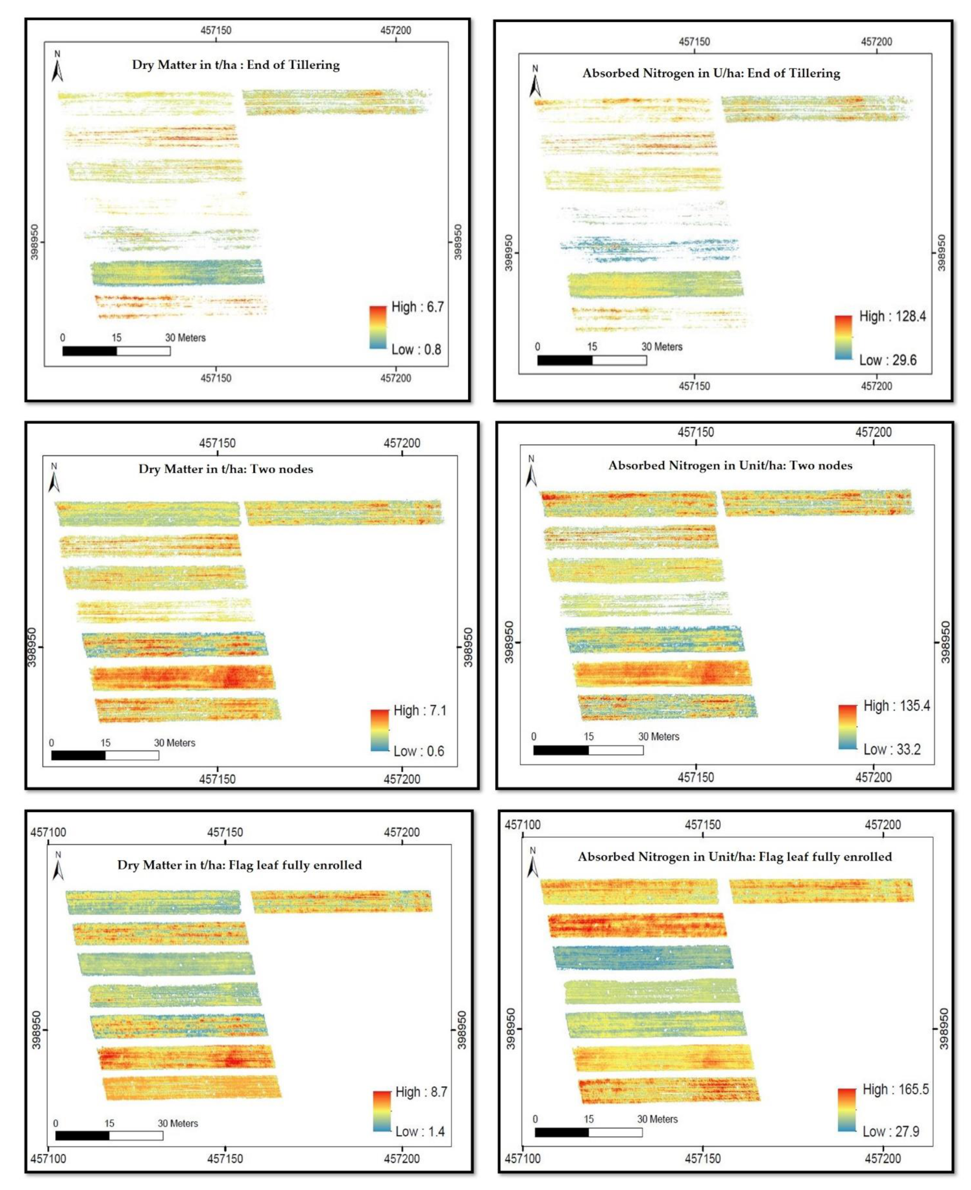
3.2. Statistical Modeling and Wheat’s Biophysical Parameters Mapping

Using the selected models of the varietal approach, maps of dry biomass, nitrogen uptake, the NNI and the difference between critical and nitrogen uptake were generated for each of the following varieties: ACHTAR, RESULTON, NAJIA, RAHMA, GUADALETTE, FAIZA, BANDERA, REMAX.

Table 4. Average of the R² and RMSE coefficients, at the level of each variety and for each index.

Vegetation Index	Linear Model				2nd Order Polynomial Model				Exponential Model
	Dry Matter		Nitrogen Uptake		Dry Matter		Nitrogen Uptake		DRY Matter		Nitrogen Uptake
	R2	RMSE	R2	RMSE	R2	RMSE	R2	RMSE	R2	RMSE	R2	RMSE
NDVI	0.229	1.182	0.240	18.795	0.511	1.012	0.478	17.479	0.337	1.115	0.172	20.899
NDRE	0.554	1.175	0.520	14.566	0.760	0.710	0.581	16.097	0.666	0.761	0.538	13.911
GNDVI	0.398	1.000	0.268	16.849	0.552	1.092	0.489	16.639	0.482	0.959	0.325	17.104
GNDRE	0.225	3.940	0.219	20.416	0.308	4.111	0.391	21.129	0.351	3.966	0.215	19.645
MTVI	0.185	1.244	0.147	20.914	0.364	1.191	0.258	19.981	0.103	1.348	0.133	18.648
RTVI	0.774	0.625	0.687	11.581	0.824	0.655	0.700	13.755	0.795	0.614	0.585	13.742
SR_NIR	0.189	1.514	0.162	20.560	0.444	1.172	0.435	18.543	0.167	1.327	0.239	19.893
SR_RE	0.736	0.661	0.619	13.055	0.794	0.651	0.702	12.349	0.763	0.659	0.600	12.138

summarizes the results of modeling determinants for each variety to estimate dry matter and nitrogen uptake by all three types of models. It represents the average of the R² and RMSE coefficients, at the level of each variety and for each index. In terms of dry matter and nitrogen uptake modeling, the RTVI index presents the best average values of R² and RMSE compared to the results of the other indices. This is interpreted by the fact that the RTVI is the more suitable index for the dry matter and nitrogen modeling operation for all the studied varieties. Therefore, RTVI is the index selected to establish the models for estimating wheat biophysical parameters studied at this project. Maps of dry matter, nitrogen uptake, NNI and the difference between critical nitrogen and nitrogen uptake were established using the vegetation index and a model selected based on R² and RMSE metrics RMSE (Figure 11).

By considering the general approach, the dry matter and nitrogen uptake models for all the varieties of the platform were estimated using linear, 2nd order polynomial and exponential regression functions considering the RTVI index. The following table (

Table 5. Values of R² and RMSE by general approach using linear and non-linear regression.

Dependent Variables	Linear Model		2nd Order Polynomial Model		Exponential Model
	R2	RMSE	R2	RMSE	R2	RMSE
Dry matter	0.761	0.63	0.741	0.67	0.690	0.67
Nitrogen uptake	0.638	12.86	0.635	12.81	0.576	14.00

) shows the R² and RMSE determination parameters for each regression model. The linear model provides the highest correlation value between the RTVI index and the dry matter as well as for the nitrogen uptake variable. Based on these models (

Table 6. Mathematical linear models of dry matter and nitrogen uptake and values of R² and RMSE by general approach.

Dependent Variables	Model	R2	RMSE
Dry matter	$0.33\times \mathrm{RTVI}-0.352$	0.761	0.63
Nitrogen uptake	$5.126\times \mathrm{RTVI}+22.202$	0.638	12.86

), the dry matter and nitrogen uptake maps were generated for all varieties at the platform and from this the Nitrogen Nutrition Index and the difference between nitrogen uptake and critical nitrogen have been established (Figure 11). When using Random Forest technique at each stage of development of wheat, we were able to retrieve R² and RMSE for the test set described in

Table 7. Values of R² and RMSE by general approach using Random Forest.

Dependent Variables	End of Tillering		Two Nodes		Last Leaf Flag Unrolled
	R2	RMSE	R2	RMSE	R2	RMSE
Dry matter	0.717	0.136	0.779	0.600	0.781	0.789
Nitrogen uptake	0.632	7.284	0.742	15.148	0.669	17.329

. Dry matter and nitrogen uptake maps were generated for the whole platform the Nitrogen Nutrition Index and the difference between nitrogen uptake and critical nitrogen were thus calculated (Figure 12).

3.3. Wheat Yield Prediction

One of the preliminary results for yield prediction is the harvest index for all the plots (Equation (6)). Thus, Figure 13 presents a diagram that compares the values of predicted yield according to both varietal and general approaches and allows to examine the differences from the harvested yield. By considering the varieties, the model allowed to estimate the yield up to 32% of the difference between the actual yield and a minimum difference of 7%. Furthermore, when using the general approach, Random Forest allowed a minimum difference of 1% and a maximum of 21% compared to the linear regression where a minimum gap of 0.2% and maximum of 29% are reached. Whereas

Table 8. Predicted wheat yield using varietal approach.

Variety	Predicted Yield (t/ha)
ACHTAR	2.934
REMAX	2.887
BANDERA	2.262
FAIZA	2.316
GUADALETTE	3.351
RAHMA	2.612
NAJIA	2.373
RESULTON	3.175

and

Table 9. Predicted wheat yield using general approach.

Variety	Harvested Yield (t/ha)	Predicted Yield (t/ha)
		Random Forest	Linear Regression
3A GHARIME BD	3.400	2.866	2.495
ACHTAR	2.754	2.828	2.248
ALBIANO	0.782	2.684	2.756
ALMANER	3.570	2.773	2.657
ATLAS	2.720	2.595	1.958
BANDERA	3.264	2.901	2.541
BT V2	4.114	3.170	2.849
BT V3	4.488	3.040	2.704
FAIZA	3.400	2.923	2.586
FARRAGE BD	3.230	3.493	3.174
FARRAS	4.624	3.281	2.946
FEELIN	1.292	2.970	2.577
GUADALETTE	2.822	2.730	2.286
GUADALIQ BD	3.740	3.011	2.667
ICAVERVE BD	3.366	3.574	3.233
IDAN 39	4.658	3.104	2.767
MARGHARITA	3.230	2.948	2.583
NACHIT BD	4.658	3.129	2.802
NAJIA	3.944	3.479	3.149
RAHMA	3.672	2.918	2.555
REMAX	3.400	2.944	2.606
RESULTON	3.570	2.869	2.500
TERBOL	2.856	2.674	2.147
TESFA	2.890	2.637	2.076

represent the values of predicted yield of wheat using both varietal and general approach as well as the actual harvested yield in t/ha.

Random Forest technique helped shorten the gap between the actual yield values and the predicted ones. The varietal approach for yield prediction did not have a large impact on the predicted values given the microplatforms size (300 m²) and therefore the limited number of extracted plots during each period (2 to 3). However, the yield prediction model can be improved by increasing the number of flights acquired from wheat leaf development (BBCH1) to heading (BBCH5) and also from heading to maturity (BBCH8). This will allow the use of the cumulative RTVI values from each flight [33]. Moreover, the HImax parameter of the model adjusted to our experimental platform can be readjusted by generalizing the extraction of the plots in order to consider the platforms having a maximum yield among all the platforms present and not only those where plots were extracted. As a result, some late varieties have a gap of up to 2.4 t/ha and others are affected by the dry year confirmed by the Ministry of Agriculture [36].

The flight schedule was related to the phenological stages of wheat development that correspond to the BBCH scale at stages 29–30, 32 and 39, respectively. These stages make it possible to monitor the accumulation of wheat’s dry matter and to ensure convenable nitrogen nutrition. Moreover, the late tillering is the stage for which the plant is able to produce tillers and therefore it can play an important role in the survival of wheat. During this stage, a strong relationship between the vegetation indices and the crop concerned is observed [37]. Additionally, flights during the two-node, last leaf flag unrolled stages allow estimation of wheat yield and dry matter [38]. However, the use of a fixed-wing drone requires a terrain with adequate take-off and landing sites. If there are obstacles in the area of the flight, safety measures must be taken to properly identify the landing locations.

4. Conclusions

The current study presents an example of the contribution of geospatial technologies in precision agriculture where UAV’s multispectral imagery is considered as an important component in monitoring and estimating crop yield. Data acquisition phase can be described as an important step within our approach based essentially on the use of UAV’s multitemporal and multispectral images as well as in-situ data, during five different phenological stages of wheat growth.

The proposed methodology aims to predict wheat’s biophysical parameters namely, dry matter, nitrogen uptake and wheat yield. By establishing statistical models, using regression and Random Forest along with RTVI vegetation index. RTVI was selected based on the results of a varietal analysis considering 12 wheat varieties and 8 vegetation indices in which it presented better results in terms of RMSE and R² values and had a better correlation with wheat biophysical parameters. Furthermore, the current methodology has enabled us to estimate a difference between actual and predicted yield of about 1 to 21% for some varieties using Random Forest technique. The difference depends mainly on both variety and the used modeling technique. However, some wheat varieties have shown a significant difference in yield between 2.6 and 3.3 t/ha.

We highlighted the role of Red-Edge band and Machine Learning techniques in the estimation of agronomic parameters of different varieties of wheat. However, certain technical and general aspects regarding the above methodology need to be considered as recommendations for future works and studies. Namely, the integration of soil parameters such as soil type, runoff, drainage and meteorological parameters such as temperature, precipitation, humidity and evapotranspiration in the estimation model in order to refine its results. We also recommend to explore and compare alternative models for direct yield estimation to increase the precision of the model in terms of difference between ground-truth yield and estimated yield values as well as to generate a model adapted to the context of national agriculture.

References

1. OECD/FAO. OECD-FAO Agricultural Outlook 2020–2029; OCDE: Paris, France; FAO: Rome, Italy, 2020. [Google Scholar] [CrossRef]
2. Ahmad, L.; Mahdi, S.S. Components of Precision Agriculture. In Satellite Farming; Springer: Berlin/Heidelberg, Germany, 2018. [Google Scholar] [CrossRef]
3. King, A. Technology: The Future of Agriculture. Nature 2017. [Google Scholar] [CrossRef] [PubMed] [Green Version]
4. Innovation—Feeding the World. Available online: http://www.fao.org/family-farming/detail/fr/c/340600/ (accessed on 29 March 2019).
5. Precision Agriculture Market Analysis by Component (Hardware, Software & Services), By Technology (Variable Rate Technology, Remote sensing, Guidance Systems), By Application, By Region, And Segment Forecasts, 2014–2025. Available online: http://www.hexareports.com/report/precision-agriculture-market (accessed on 17 April 2019).
6. Wahab, I.; Hall, O.; Jirström, M. Remote sensing of yields: Application of UAV imagery-derived ndvi for estimating maize vigor and yields in complex farming systems in Sub-Saharan Africa. Drones 2018, 2, 28. [Google Scholar] [CrossRef] [Green Version]
7. Messina, G.; Modica, G. Applications of UAV Thermal Imagery in Precision Agriculture: State of the Art and Future Research Outlook. Remote Sens. 2020, 12, 1491. [Google Scholar] [CrossRef]
8. Tao, H.; Feng, H.; Xu, L.; Miao, M.; Yang, G.; Yang, X.; Fan, L. Estimation of the Yield and Plant Height of Winter Wheat Using UAV-Based Hyperspectral Images. Sensors 2020, 20, 1231. [Google Scholar] [CrossRef] [PubMed] [Green Version]
9. Balaghi, R.; Jlibene, M.; Tychon, B.; Eerens, H. Preface. In Prediction Agrometeorologique des Rendements Cerealiers au Maroc; National Institute for Agronomic Research of Morocco-INRA: Rabat, Morocco, 2012; pp. 1–10. [Google Scholar]
10. Rehman, A.; Ahsan, M.; Latif, M.; Naseer, A. Mapping Wheat Crop Phenology and the Yield using Machine Learning (ML). Int. J. Adv. Comput. Sci. Appl. 2018, 9, 301–306. [Google Scholar]
11. Tuvdendorj, B.; Wu, B.; Zeng, H.; Gantsetseg, B.; Nanzad, L. Determination of Appropriate Remote Sensing Indices for Spring Wheat Yield Estimation in Mongolia. Remote Sens. 2019, 11, 2568. [Google Scholar] [CrossRef] [Green Version]
12. Hassan, M.; Yang, M.; Rasheed, A.; Yang, G.J.; Reynolds, M.; Xia, X.; Xiao, Y.; He, Z. A rapid monitoring of NDVI across the wheat growth cycle for grain yield prediction using a multi-spectral UAV platform. Plant Sci. 2018. [Google Scholar] [CrossRef] [PubMed]
13. Guan, S.; Fukami, K.; Matsunaka, H.; Okami, M.; Tanaka, R.; Nakano, H.; Sakai, T.; Nakano, K.; Ohdan, H.; Takahashi, K. Assessing Correlation of High-Resolution NDVI with Fertilizer Application Level and Yield of Rice and Wheat Crops Using Small UAVs. Remote Sens. 2019, 11, 112. [Google Scholar] [CrossRef] [Green Version]
14. Mesas-Carrascosa, F.-J.; Torres-Sánchez, J.; Clavero-Rumbao, I.; García-Ferrer, A.; Peña, J.-M.; Borra-Serrano, I.; López-Granados, F. Assessing Optimal Flight Parameters for Generating Accurate Multispectral Orthomosaicks by UAV to Support Site-Specific Crop Management. Remote Sens. 2015, 7, 12793–12814. [Google Scholar] [CrossRef] [Green Version]
15. Coombes, M.; Fletcher, T.; Chen, W.-H.; Liu, C. Optimal Polygon Decomposition for UAV Survey Coverage Path Planning in Wind. Sensors 2018, 18, 2132. [Google Scholar] [CrossRef] [PubMed] [Green Version]
16. Cabreira, T.M.; Brisolara, L.B.; Ferreira, P.R., Jr. Survey on Coverage Path Planning with Unmanned Aerial Vehicles. Drones 2019, 3, 4. [Google Scholar] [CrossRef] [Green Version]
17. Jürgen, M. Analyse de Référence Selon la Méthode de Dumas ou la Méthode de Kjeldahl? Comparaison des Méthodes et Considérations pour L’analyse de L’azote/des Protéines dans les Denrées Alimentaires et les Aliments pour Animaux; Livre Blanc de FOSS; FOSS: Hilleroed, Denmark, 2017; Volume 1, pp. 1–5. [Google Scholar]
18. Radiometric Calibration Target. Available online: https://support.pix4d.com/hc/en-us/articles/206494883-Radiometric-calibration-target (accessed on 18 June 2019).
19. Xu, K.; Gong, Y.; Fang, S.; Wang, K.; Lin, Z.; Wang, F. Radiometric Calibration of UAV Remote Sensing Image with Spectral Angle Constraint. Remote Sen. 2019, 11, 1291. [Google Scholar] [CrossRef] [Green Version]
20. Pix4D Mapper User Manual. 2017. Available online: https://support.pix4d.com/hc/en-us/articles/204272989-Offline-Getting-Started-and-Manual-pdf (accessed on 29 March 2019).
21. Visockiene, J.S.; Domantas, B.; Ugnius, R. Comparison of UAV images processing softwares. J. Meas. Eng. 2014, 2, 111–121. [Google Scholar]
22. eCognition User Manual. 2019. Available online: https://docs.ecognition.com/v9.5.0/eCognition_documentation (accessed on 17 April 2019).
23. Hamilton, R.; Megown, K.; Mellin, T.; Fox, I. Guide to Automated Stand Delineation Using Image Segmentation; Report Number: RSAC-0094-RPT1; US Forest Service, Remote Sensing Applications Center: Salt Lake City, UT, USA, 2007. [Google Scholar]
24. Fu, Z.; Jiang, J.; Gao, Y.; Krienke, B.; Wang, M.; Zhong, K.; Cao, Q.; Tian, Y.; Zhu, Y.; Cao, W.; et al. Wheat Growth Monitoring and Yield Estimation based on Multi-Rotor Unmanned Aerial Vehicle. Remote Sens. 2020, 12, 508. [Google Scholar] [CrossRef] [Green Version]
25. Liakos, K.G.; Busato, P.; Moshou, D.; Pearson, S.; Bochtis, D. Machine Learning in Agriculture: A Review. Sensors 2018, 18, 2674. [Google Scholar]
26. Han, S.; Kim, H. On the Optimal Size of Candidate Feature Set in Random forest. Appl. Sci. 2019, 9, 898. [Google Scholar] [CrossRef] [Green Version]
27. Scikit Learn Documentation. Available online: https://scikit-learn.org/stable/modules/ensemble.html#forest (accessed on 3 March 2019).
28. Anaconda Documentation. Available online: https://docs.anaconda.com/anaconda/install/ (accessed on 19 May 2019).
29. Malik, U. Random Forest Algorithm with Python and Scikit-Learn. Available online: https://stackabuse.com/random-forest-algorithm-with-python-and-scikit-learn/ (accessed on 25 April 2019).
30. Justes, E.; Mary, B.; Meynard, J.M. Evaluation of a nitrate test indicator to improve the nitrogen fertilization of winter wheat crops. Commun. Soil Sci. Plant Anal. 1995, 34, 2539–2551. [Google Scholar]
31. Stafford, J.V. Precision Agriculture ’05; European Conference on Precision Agriculture; Wageningen Academic Publishers: Wageningen, The Netherlands, 2005; Available online: http://0-public-ebookcentral-proquest-com.brum.beds.ac.uk/choice/publicfullrecord.aspx?p=3572015 (accessed on 12 June 2019).
32. Raun, R.; Solie, J.B.; Johnson, G.V. Improving Nitrogen Use Efficiency in Cereal Grain Production with Optical Sensing. Agron. J. 2001, 94, 815–820. [Google Scholar] [CrossRef] [Green Version]
33. Zhang, H. The model of wheat yield forecast based on modis-ndvi. ISPRS Ann. Photogramm. Remote Sens. Spat. Inf. Sci. 2012, I-7, 1–4. [Google Scholar]
34. Whitbread, A.; Hancock, J. Estimating grain yield with the French and Schultz approaches vs simulating attainable yield with APSIM on the Eyre Peninsula. In Proceedings of the 14th Agronomy Conference, Adelaide, Australia, 21–25 September 2008. [Google Scholar]
35. Marché Agricole des Céréales. Available online: www.terre-net.fr/marche-agricole (accessed on 22 April 2019).
36. GIEWS—Global Information and Early Warning System. Available online: http://www.fao.org/giews/countrybrief/country.jsp?code=MAR (accessed on 15 March 2019).
37. Beuerlein, J.E. Wheat Growth Stages and Associated Management; The Ohio State University Extension: Columbus, OH, USA, 2001. [Google Scholar]
38. Geng, H.; Beecher, B.; He, Z.; Morris, C.F. Physical Mapping of Genes in Wheat using ‘Chinese Spring’ Chromosome Group 7 Deletion Lines. Crop Sci. 2012, 52, 2674–2678. [Google Scholar] [CrossRef]
Figure 1. The general methodology used throughout this study.
Agriengineering 03 00003 g001
Figure 2. Field site of the experimental platform 07 of domain HAMMA (Google Maps, 2019).
Agriengineering 03 00003 g002
Figure 3. Experimental platform 07 (DW: durum wheat—BW: bread wheat).
Agriengineering 03 00003 g003
Figure 4. (a) eBee Classic; (b) Airinov MultiSPEC 4C camera (Sensefly; Airinov).
Agriengineering 03 00003 g004
Figure 5. (a) MultiSPEC 4C Calibration target; (b) Image taken on the field during the calibration process.
Agriengineering 03 00003 g005
Figure 6. (a) Created mask for the experimental plots, (b) the result of plots’ extraction.
Agriengineering 03 00003 g006
Figure 7. Result of microplatforms’ extraction by OBIA (Object-based Image Analysis) approach.
Agriengineering 03 00003 g007
Figure 8. Iterative method for determining the number of trees n_estimators of Random Forest.
Agriengineering 03 00003 g008
Figure 9. Vegetation index maps (a) SR-NIR; (b) SR-RE; (c) MTVI2; (d) RTVI; (e) NDRE; (f) NDVI; (g) GNDRE; (h) GNDVI during flag leaf fully unrolled stage before sampling.
Agriengineering 03 00003 g009
Figure 10. Variation of dry matter by each vegetation index.
Agriengineering 03 00003 g010
Figure 11. Dry matter and nitrogen uptake using varietal approach during end of tillering, two nodes and flag leaf fully enrolled stages.
Agriengineering 03 00003 g011
Figure 12. Dry matter, nitrogen uptake, NNI, and difference between critical nitrogen and nitrogen uptake maps during end of tillering, two nodes and last leaf flag unrolled using (a) linear regression and (b) using Random forest.
Agriengineering 03 00003 g012