Article

Novel Route Planning Method to Improve the Operational Efficiency of Capacitated Operations. Case: Application of Organic Fertilizer

by
Mahdi Vahdanjoo
1,* and
Claus G. Sorensen
2
1
Department of Agroecology, Aarhus University, 8830 Tjele, Denmark
2
Department of Electrical and Computer Engineering, Aarhus University, 8830 Tjele, Denmark
*
Author to whom correspondence should be addressed.
Submission received: 27 May 2021 / Revised: 22 June 2021 / Accepted: 26 June 2021 / Published: 30 June 2021

Abstract

:
A field area coverage-planning algorithm has been developed for the optimization and simulation of capacitated field operations such as the organic fertilizer application process. The proposed model provides an optimal coverage plan, which includes the optimal sequence of the visited tracks with a designated application rate. The objective of this paper is to present a novel approach for route planning involving two simultaneous optimization criteria, non-working distance minimization and the optimization of application rates, for the capacitated field operations such as organic fertilizer application to improve the overall operational efficiency. The study and the developed algorithm have shown that it is possible to generate the optimized coverage plan based on the required defined capacity of the distributer. In this case, the capacity of the distributer is not considered a limiting factor for the farmers. To validate this new method, a shallow injection application process was considered, and the results of applying the optimization algorithm were compared with the conventional methods. The results show that the proposed method increase operational efficiency by 19.7%. Furthermore, the applicability of the proposed model in robotic application were demonstrated by way of two defined scenarios.

1. Introduction

Agricultural field area coverage planning enhances the efficiency of commercial auto-steering or navigation-aid systems on agricultural machines [1,2,3]. Area coverage plans provide a path that visits all points of a targeted spatial environment under the criterion of minimization of unproductive time or traveled distance and avoiding machine maneuvering in the already worked area or cropping area [4,5]. The benefits of area coverage planning include optimized driving patterns, reduced overlaps and skips, reduced soil compaction, and overall enhanced efficiency of agricultural machines [6,7]. As an example of area coverage planning, B-patterns [8] algorithmically find the optimal order of field working areas to minimize the non-working traveled distance by the agricultural vehicle. Hameed et al., 2011 [9] presented an algorithmic approach to determine the optimal driving angle and sequence of tracks under the criterion of minimizing the operational time and the amount of overlapped covered areas.
Agricultural capacitated field operations denote the type of operations that transport material in and out of the field. Examples of these operations include planting, spraying, fertilizing, or removing material from the field such as harvesting. In these operations, due to the limitation of machine load capacities, there are capacity constraints related to the materials that should be carried by the vehicle. Therefore, in order to complete the task in capacitated operations, machines need to visit the depot and return to the field several times for refilling or unloading. Several coverage planning methods for the agricultural field have been recently developed [10,11,12]. However, the case of capacitated operations has not been explicitly examined due to the complexity of consecutive decision-making related to the in-field driving actions of these operations. For instance, in the case of a fertilizing operation, when the distributer is positioned in the middle of a track and a reloading action is required (e.g., the tanker become empty and it is urgent to revisit the depot for refilling), then there are various options open to the machine’s operator to either continue in the same direction in that track to reach to the headland part and then go back to the depot or the operator can do a U-turn (180-degree turn) and go to an adjacent unworked track to return to the depot. In these studies [1,4,13,14], the capacitated field operations casted into the examples of vehicle routing problem (VRP). They showed that the agricultural fleet management problem could be expressed as the traversal of weighted graphs under some operational constraints. These papers [15,16] proposed a practical planning approach for harvesting a field with several capacitated combine harvesters and transport units. References [17,18,19] provided a route planning approach for the operations of agricultural machines in order to reduce the risk of soil compaction in the field. Jensen et al. (2015) [20] presented an algorithmic method for the optimization of capacitated field operations using the case of liquid fertilizing. The algorithm consists of two optimization parts. In the first main part, the optimal sequence of pre-defined driving actions is obtained using a state space search technique, which minimizes the non-productive traveled distance during the operation’s interruption for refilling and the corresponding resuming of the operation. In the second post-processing part, the optimal track sequence is found using the traveling salesman problem methodology, which minimizes the nonproductive traveled distance during the headland turnings.
The objective of this paper is to provide a novel approach with two optimization criteria, distance minimization and the optimization of application rates, for the capacitated field operations such as organic fertilizer application to improve operational efficiency. Different elements of the organic fertilization operation were considered in the algorithm to determine the optimal coverage plan for the agricultural field based on the capacity of the applied machine. The presented approach has two parts. In the first part, the field is represented geometrically where the boundary of the field and headland area are shown as polygons and the main cropping areas are partitioned with straight work areas (tracks) according to the defined reference line (usually the longest edge of the field). In the second part, the algorithm will find the optimal sequence of the tracks with a designated application rate for each track while minimizing the total non-working traveled distance and optimizing the application rate for all the tracks.

2. Materials and Methods

The main task in a manure distributing operation is to cover the crop area of the field with the required amount of fertilizer according to the agronomical and environmental norms. Due to the nature of capacitated operations, in order to complete the task, the depot should be visited several times for refilling, and in manure distributing operations, usually farmers prefer to visit the depot with an empty tank. Therefore, the capacity of the distributer is an important factor in generating a coverage plan for a field. The proposed algorithm in this paper will entail a solution based on the fixed capacity of the distributer regardless of the size of the field. In cases that the demand of a track is more than the capacity of the slurry distributer, by considering the extension action (adjusting the application rate of a track, to be sure that it is possible to cover it by one load) [6], the algorithm divided those tracks into smaller parts, which can be covered with one load. Moreover, the optimized application rate for each part is calculated by the algorithm and all the turnings are limited to the headland part.

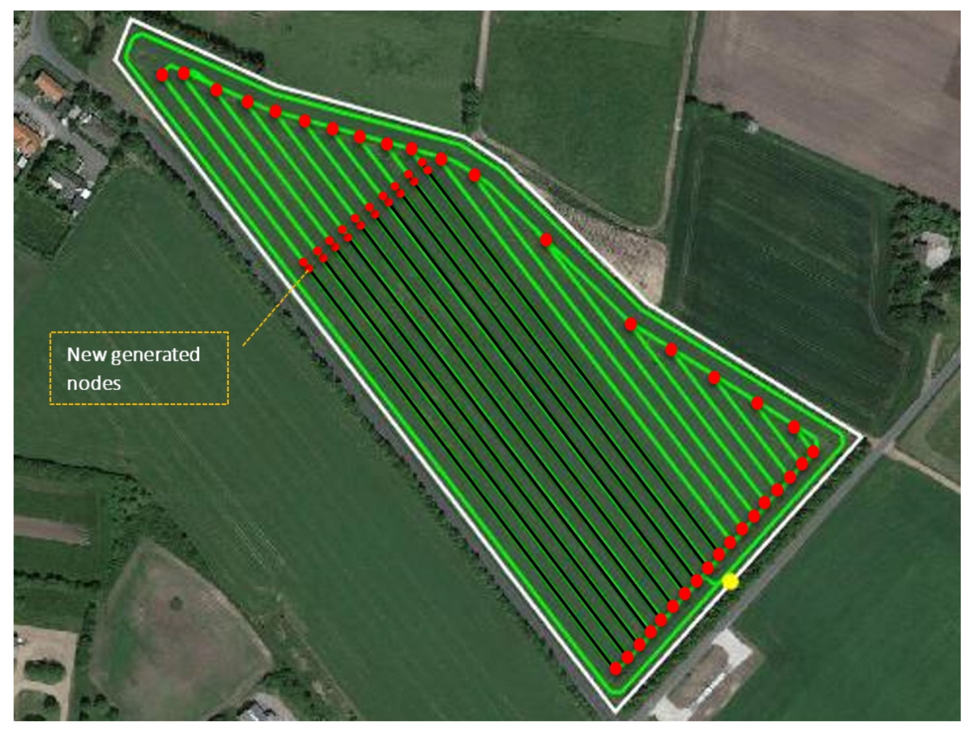
2.1. Division Action

The vehicle’s load capacity, as an important factor, has effects on the operational efficiency of the capacitated operations. Sometimes, due to the small capacity of the machine, it is not possible to completely cover a track with one load even by considering the extension action. Division action is used as a solution in this study to overcome this problem. In this action, a long track has been divided into smaller parts, which are able to be covered by the vehicle concerning the extension action. The black lines in Figure 1 refer to the parts where the r maximum extension is equal to the capacity of the tanker. The following criteria should be considered to generate the list of long tracks:
Track_max_extension = Track’s demand × (1−%P)
If the amount of maximum extension for a track is higher than the amount of vehicle’s load capacity, then that track considered as a long track and then added to a list. Then the following action is considered for each track in the list of long tracks to determine the number of divisions:
Number of divisions = Ceil (Track_max_extension/Vehicle Capacity)

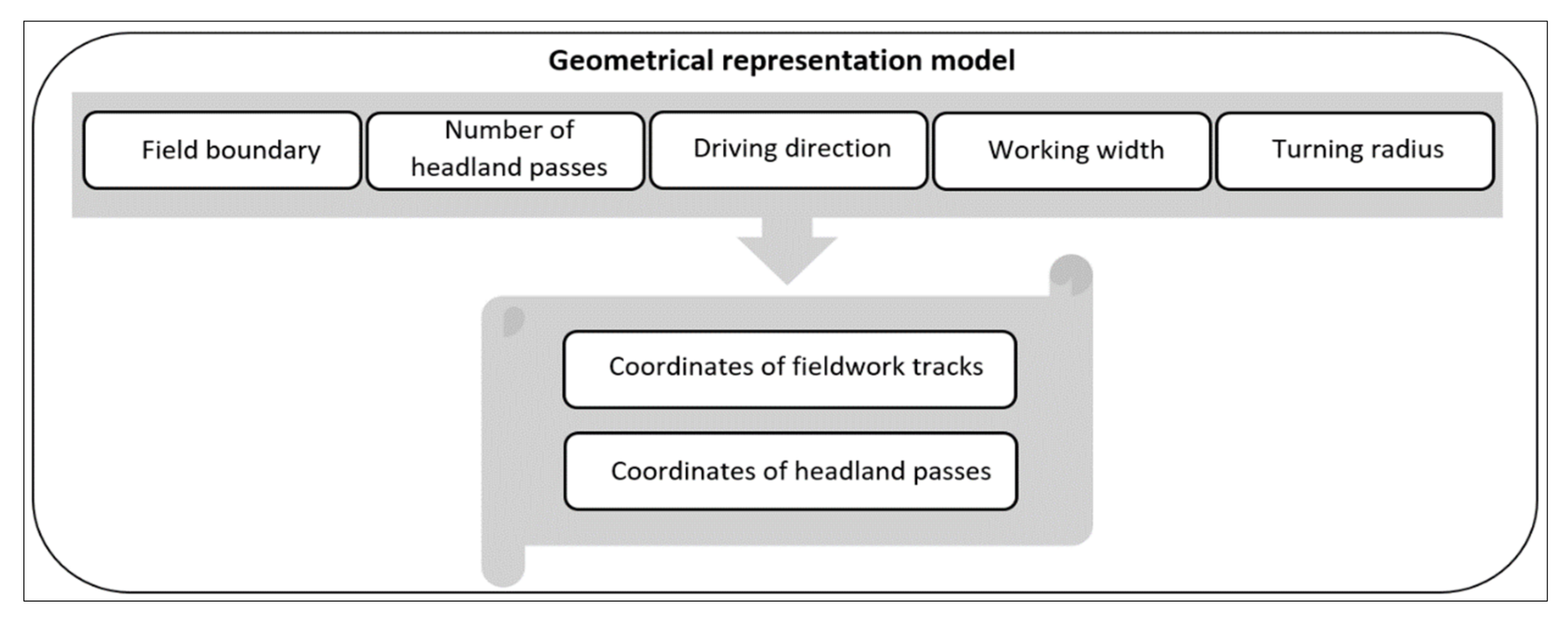
2.2. Geometrical Representation Model

The first stage of the proposed method concerns the geometrical representation of the field to generate predetermined fieldwork tracks by applying geometrical primitives such as points, lines, and polygons. The outputs of the first stage as showed in Figure 2 are a set of line segments or polylines representing the fieldwork areas and headland passes that can be followed by the vehicle [4].

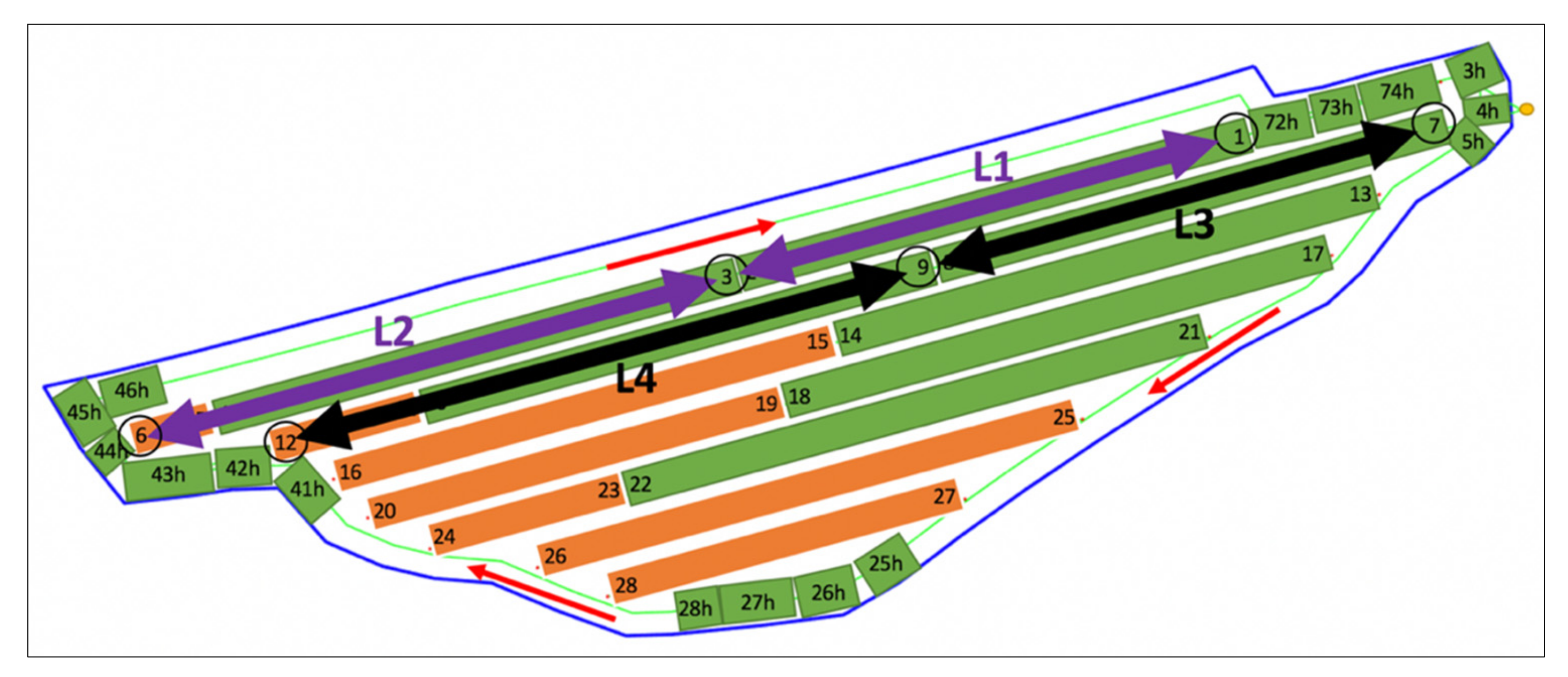
2.3. Cost Matrix Generation

After dividing the long tracks into smaller parts, two new nodes are generated for each part. These new nodes should be added to the field graph and the cost matrix should be updated based on them. According to Figure 3, the original cost matrix includes the nodes (0, 1, 6, 7, 12, 13, 16, 17, 20, 21, 24, 25, 26, 27, 28), and it shows the distances of these nodes from each other. For example, after adding the node 3, the distance from this node to the others can be determined by adding the length L1 to the values in the column corresponding to the node 1 in the original cost matrix [6]. The length L2 is not considered due to this rule that the orange parts are going to be covered at the beginning and in this study, it is not allowed to reach to a node by crossing a pre-applied area with a full tanker. Moreover, the distance between two new nodes such as nodes 3 and 9 can be calculated by adding the length (L1 + L3) to the distance of the nodes 1 and 7 from each other.

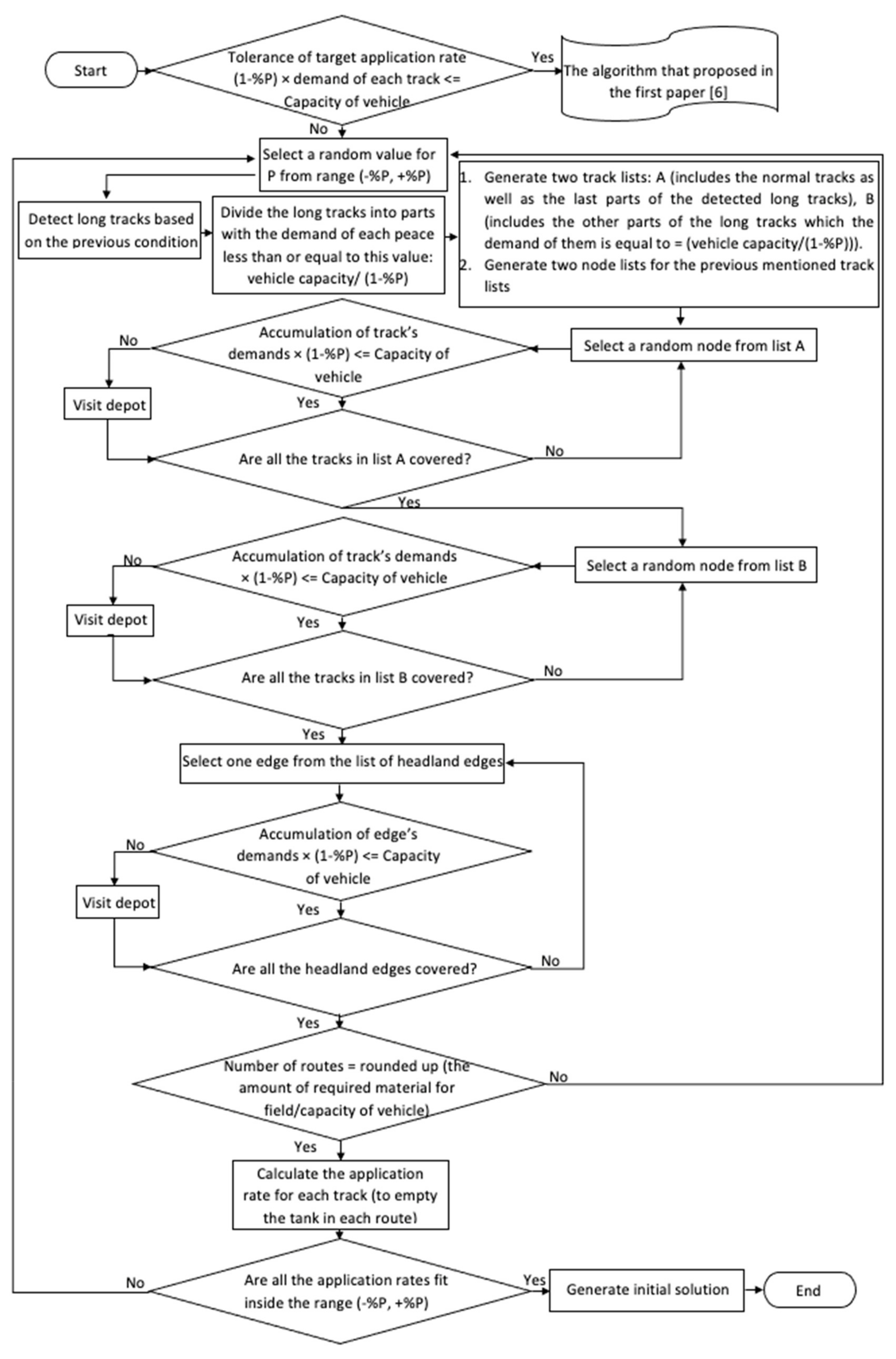
2.4. Optimization Algorithm

The problem explored in this study is to find the optimal traversal sequence of fieldwork tracks with minimum non-working distance together with the adjusted application rate for each track. Since there is a large discrete search space in this problem, it can be classified as a well-known VRP NP-hard (non-deterministic polynomial-time) problem where tracks are covered instead of customers and vehicles could refill at the depot. The meta-heuristic algorithm Simulated Annealing (SA) is applied to approximate the global optimum for this problem. A new solution in the SA algorithm is generated by applying various neighborhood operators on an initial solution [6]. In order to make an initial solution, in the first step, the algorithm places the orange parts (Figure 3) into groups which can be covered by one load. Then the green parts (which can each be covered by one load) will be added to the initial solution, and at the end, the headland parts are added to complete the coverage plan. The following flowchart (Figure 4) represents an overview of the process of generating an initial solution.
The geometrical representation model partitioned the field and generated the fieldwork tracks with their corresponding demand. Then the algorithm checks if all the tracks can be covered based on the capacity of the spreader by considering this criterion: (1- tolerance from target application rate) × track’s demand <= capacity of spreader. If all the tracks fit in this criterion, then algorithm will generate an initial solution according to the first paper [6]. Otherwise, it will select a random value for the tolerance from target application rate from the range (−%P,+%P). Then, based on the selected %P, it will apply the previous criterion to detect the long tracks. Then, based on the formula number 1, it will divide the long tracks into some parts. Then, two lists of tracks will be generated. The first group ‘A’ includes the normal tracks as well as the last part of the detected long tracks (the orange parts in the Figure 3). The second group ‘B’ includes the other parts of the long tracks (the green parts in the Figure 3). Then it will randomly select one track, and then check the following capacity criterion: (Accumulation of track’s demand × (1−%P) <= spreader’s capacity). If the track’s demand fits into the previous criterion, then it will check if all the tracks in group ‘A’ is covered or not. This loop is going to continue until the demand of the added track will not fit in the capacity criterion. Then, the refilling process (visit to depot) will happen, and after that, the algorithm checks if all the tracks in group ‘A’ are covered or not. After covering all the tracks in group ‘A’, the algorithm takes a random track from group ‘B’. The same procedure will be applied until all the tracks inside the group ‘B’ are covered. Then, the headland edges are going to be added to the solution by considering the same procedure. Then the number of routes (trips) should be equal to the ceil (the amount of required fertilizer for the field/distributer capacity) to be sure to visit the depot with empty tanker. Then, the application rate for each track will be calculated and checked to see if they fit into the range ±%P of the target application rate; otherwise, the algorithm will start again by choosing a random value for P.

3. Results

In the first part of the results, the proposed algorithm is compared with the conventional method applied by the farmers to show the improvement in operational efficiency caused by using this algorithm. A trailing hose fertilizing operation was performed and recorded. The GPS data gathered by the machine were plotted in MATLAB® software (version R2018b).
Figure 5 geometrically represents the sample field 1, and Figure 6 demonstrates how farmers performed the slurry application on that field. Based on the recorded data, the total distance traveled by the machine in the conventional method is 96,009 m, which 8359 m of that are productive and 87,650 is unproductive distance.
The input parameters applied in the model showed in the Table 1 and by using the proposed method the optimal coverage plan was generated and the results were showed in the Table 2.
In order to have a complete comparison, the traveled distance and time from the gate to the depot and back to the gate is calculated equaling 3100 m and 11.7 min. This distance should be added to the result of the simulation model for the traveled non-working distance. Figure 7 depicts the optimized coverage plan generated by applying the proposed method in this study. The output of the optimization algorithm is an optimal coverage plan that is used to generate a log file by applying the simulation model. At the end, the total non-working traveled distance and time calculated and presented as the results of the simulation model.
According to the Table 2, in the optimized coverage plan, there are 17 routes, which means that the depot should be visited 17 times to complete the operation. Therefore, to calculate the total non-working distance, 17 should be multiplied to the value of the distance from the gate to the depot and back to the gate, and then this amount should be added to the results of the simulation model.
The results of the simulation model for the optimized plan showed that the non-working traveled distance is about 17,645 m, and by adding the amount 52,700 (17* 3100 m) to that, the total non-working distance for the optimized plan is 70,345 m. Based on the presented comparison between the optimized and conventional plan in the Table 3, applying the proposed algorithm increases the operational efficiency for the farmers by 19.7%.
In the second part of the results, to show the benefits of the proposed algorithm in this study, the method presented by Jensen, Bochtis, and Sørensen (2015) was considered for comparison. The properties of the distributer that was used in the shallow injection fertilizing operation (Operation B) were presented in the Table 4.
The presented data for the fertilizing operation were applied as an input for the simulation model. The results of the simulation model for covering the sample field with the mentioned distributer were demonstrated in the Table 5 and Figure 8 presented the output of the geometrical representation model, (a) for a normal slurry distributer, and (b) for robotic application. The list of application rates for each edge ID presented in the Table A1, Appendix A.
As the benefits of the presented algorithm in this study, it is possible to generate the optimized coverage plan for the robotic application with very small capacity. Two scenarios were defined for the robotic application based on either by crossing from the wet area or by avoiding that. Table 6 shows the generated solution for the first scenario which avoids passing the robots from the wet parts of the field with full tank. The solution is an optimized field coverage plan for a fleet of robots (three robots) by considering two depots for the sample field. The list of application rates for each edge ID presented in the Table A2.
In the second scenario, due to this fact that the weight of the robot is much lighter than a big slurry distributer, it is possible to cross the wet area with the robots only at the end of the tracks (the orange parts, demonstrated in Figure 8b) and only one time. Table 7 shows the generated solution for the second scenario and the outputs of the simulation model.
In order to calculate the total time of the fertilizing process, the travel time should be added to the working time. Due to this fact that three robots work simultaneously, therefore, the total time for the process can be determine as the maximum operation time between robots. The total operation time for the normal slurry distributer is 48.94 min (43.3 + 5.64). For the robotic solution in the first scenario, the total operational time is equal to 55.68 min (37.55 + 18.13) and for the second scenario it is equal to 38.38 min (20.08 + 18.3).
Figure 9 demonstrates the comparison between robotic solutions with a normal slurry distributer. The comparison of the total working and non-working distance shows that the big slurry distributer has less total working and non-working distance in comparison with robotic solutions due to the fact that the working width of the normal distributer machine is 2.6 times bigger than the working width of the robots. Moreover, the comparison of the total operation time between the normal slurry distributer and the robotic application shows that the big slurry distributer can complete the operation faster than the first scenario of the robotic application (6.74 min earlier). However, by considering the second scenario (robotic solution), it is possible to finish the operation faster than the normal slurry distributer (10.56 min earlier).

4. Discussion

The proposed algorithm in this paper will entail a solution based on the fixed capacity of the distributer regardless of the size of the field. The algorithm avoids the turnings in the main cropping area of the field and by limiting all the turnings to the headland part it can reduces the amount of soil compaction in the field. As presented in the result part, the proposed algorithm results in 19.7% efficiency, which means that in the optimized solution, the amount of traveled distance is 17,305 (m) less than the conventional method. By assuming the amount of fuel consumption and the working speed for the distributer equal to 30 (liter/hour) and 6 (km/hour) respectively, it is possible so save 86.5 L of fuel during the operation. Consequently, as the benefit of this saving in the fuel consumption, there are less Greenhouse Gases (GHG) emissions during the operation. Moreover, it is possible to generate the optimized coverage plan for the robotic application with very small capacity.
Robotic application as a solution can significantly increase the efficiency of conventional farming activities where operations are manually conducted by farmers. They can reduce the requirements for manpower and workload, including skilled machine operators, by performing the tasks automatically [21]. The application of robots in precision fertilizing operations can provide the optimal amount of nutrients to the crops at a proper time and position, which consequently can reduce the percentage of agricultural inputs and the environmental impacts [22].
The capacity of a distributer is an important factor that can affect the amount of traveled non-working time and distance in the field. Distributers with bigger tanks can cover more tracks in one load and they can complete the field tasks in a smaller number of trips to the depot for refilling. However, bigger distributers are heavier than a small robot and they can increase the risk of soil compaction in the covered parts of the field [18]. Moreover, autonomous robots have less operations cost due to this fact that they need less supervision.
The working width of a distributer is another effective factor that can change the amount of traveled non-working time and distance in the field. Distributers with wider working widths can cover bigger areas while operating. Therefore, increasing the working width of the spreader can reduce the total non-working traveled distance in the field. Moreover, the tolerance from target application rate is regulated automatically based on the velocity of the spreader by the electro-hydraulic control system.
Due to the dynamic and complexity of the agricultural environments, applying a robotic solution in this unstructured environment requires advanced technology. Autonomous robots are not able to respond to unpredictable events and operating in variable environments complicates the robotic application [23]. Another challenge in applying robotic solutions in agriculture is related to the seasonality of agriculture, which makes it difficult for robotic systems to reach to the same level of deployment in manufacturing. Limited capacity and working width of agricultural robots required them to travel more distances to complete their field tasks. Considering a fleet of homogenous robots as well as locating some buffer tanks (as depots) in different parts of the field can be used as a solution to overcome those limiting factors and reach to the same efficiency as the normal agricultural machineries. The amount of fuel/energy consumption is also important to consider. To compete with big machines, the robots need to be more efficient in fuel or energy consumption due to this fact that they are small and they need to travel greater distances in the field. Moreover, some agricultural operations such as ploughing are so energy demanding that applying robotic solution for these kinds of operations is still a challenge.
In development of an agricultural robots, several considerations required such as developing advance algorithms for controlling, planning, and sensing. Moreover, they need to operate in different conditions such as in wet environments without getting stuck or destroying the soil structure [22].
In future research, the robotic solution will be considered for other agricultural operations and their operational efficiency will be compared with the normal machineries in the field. Moreover, additional studies require to investigate the fuel consumption and GHG emissions of these robots and compare them with normal agricultural machineries.

5. Conclusions

The proposed model generates a coverage plan, which can be used for capacitated field operations. The model consists of two parts: optimization and simulation algorithms. In the optimization algorithm, the Simulated Annealing (SA) is applied to determine the optimal traversal sequence of fieldwork tracks under the criterion of minimizing the non-working traveled distance during the headland turnings with appropriate application rate for each track. Moreover, the simulation algorithm generated the division of the task time and traveled distance for each element (productive/non-productive) of the operation. The operations efficiency of the optimized plans generated by the proposed method in this study was compared with the conventional methods used by farmers. Results show that applying the proposed model can bring a 19.7% increase in operational efficiency and reduce the non-working traveled distance and time. The proposed algorithm can be used as a tool to improve the operational efficiency of the capacitated operations such as slurry applications. As the benefits of the presented algorithm in this study, it is possible to generate the optimized coverage plan for the robotic application with a very small capacity.

Author Contributions

Conceptualization, M.V. and C.G.S.; methodology, M.V. and C.G.S.; software, M.V.; validation, M.V. and C.G.S.; formal analysis, M.V.; investigation, M.V.; resources, C.G.S.; data curation, M.V.; writing—original draft preparation, M.V.; writing—review and editing, M.V. and C.G.S.; visualization, M.V.; supervision, C.G.S.; project administration, C.G.S.; funding acquisition, C.G.S. All authors have read and agreed to the published version of the manuscript.

Funding

This research received no external funding.

Institutional Review Board Statement

Not applicable.

Informed Consent Statement

Not applicable.

Data Availability Statement

Data sharing not applicable.

Conflicts of Interest

The authors declare no conflict of interest.

Appendix A

Table A1. The list of application rates for covering the sample field with a normal distributer (capacity 24 m3).
Node/Edge IDApplication Rate
(liter/m2)
Node/Edge IDApplication Rate
(liter/m2)
1,21.067‘62h’0.899
3,4 1.067‘63h’0.899
5,6 1.067‘64h’0.899
7,8 1.067‘65h’0.899
9,10 1.067‘66h’0.899
11,12 1.067‘67h’0.899
13,14 0.995‘68h’0.899
15,16 0.995‘69h’0.899
17,18 0.995‘70h’0.899
19,20 0.995‘71h’0.899
21,22 0.995‘72h’0.899
23,24 0.995‘73h’0.899
25,260.995‘74h’0.899
27,28 0.995‘75h’0.899
29,300.995‘76h’0.899
31,32 0.995‘77h’0.899
‘3h’0.899‘78h’0.899
‘4h’ 0.899‘79h’0.899
‘5h’ 0.899‘80h’0.899
‘6h’ 0.899‘81h’0.899
‘7h’ 0.899‘82h’0.899
‘8h’0.899‘83h’0.899
‘9h’0.899‘84h’0.899
‘10h’ 0.899‘85h’0.899
‘11h’ 0.899‘86h’0.899
‘12h’ 0.899‘87h’0.899
‘13h’ 0.899‘88h’0.899
‘14h’ 0.899‘89h’0.899
‘15h’0.899‘90h’0.899
‘16h’0.899‘91h’0.899
‘17h’0.899‘92h’0.899
‘18h’0.899‘93h’0.899
‘19h’0.899‘94h’0.899
‘20h’ 0.899‘96h’0.899
‘21h’0.899‘97h’0.899
‘22h’0.899‘98h’0.899
‘23h’0.899‘99h’0.899
‘24h’ 0.899‘100h’0.899
‘25h’ 0.899‘101h’0.899
‘26h’0.899‘102h’0.899
‘27h’0.899‘103h’0.899
‘28h’0.899‘104h’0.899
‘29h’0.899‘105h’0.899
‘30h’0.899‘106h’0.899
‘31h’0.899‘107h’0.899
‘32h’0.899‘108h’0.899
‘33h’0.899‘109h’0.899
‘34h’0.899‘110h’0.899
‘35h’0.899‘111h’0.899
‘36h’0.899‘112h’0.899
‘37h’0.899‘113h’0.899
‘38h’0.899‘114h’0.899
‘39h’0.899‘115h’0.899
‘40h’0.899‘116h’0.899
‘41h’ 0.899‘117h’0.899
‘42h’0.899‘118h’0.899
‘43h’ 0.899‘119h’0.899
‘44h’0.899‘120h’0.899
‘45h’0.899‘121h’0.899
‘46h’ 0.899‘122h’0.899
‘47h’ 0.899‘123h’0.899
‘48h’0.899‘124h’0.899
‘49h’0.899‘125h’0.899
‘50h’0.899‘126h’0.899
‘51h’ 0.899‘127h’0.899
‘52h’ 0.899‘128h’0.899
‘53h’0.899‘129h’0.899
‘54h’0.899‘130h’0.899
‘55h’0.899‘131h’0.899
‘56h’0.899‘132h’0.899
‘57h’0.899‘133h’0.899
‘58h’ 0.899‘134h’0.899
‘59h’0.899‘135h’0.899
‘60h’0.899‘136h’0.899
‘61h’0.899‘137h’0.899
Table A2. The list of application rates for covering the sample field with a homogeneous fleet of robots (capacity 0.8 m3).
Node/Edge IDApplication Rate
(liter/m2)
Node/Edge IDApplication Rate
(liter/m2)
3,41.020‘35h’ 0.708
5,6 0.912‘36h’ 0.708
7,8 1.020‘37h’ 0.708
9,10 0.912‘38h’ 0.708
11,12 1.020‘39h’ 0.708
13,14 1.271‘40h’ 0.708
15,16 1.020‘41h’ 0.708
17,18 1.271‘42h’0.708
19,20 1.020‘43h’ 0.708
21,22 0.892‘44h’ 0.708
23,241.020‘45h’ 0.708
25,26 0.892‘46h’ 0.708
27,28 1.020‘47h’ 0.708
29,30 0.892‘48h’ 0.708
31,32 1.020‘49h’ 0.708
33,34 0.953‘50h’ 0.708
35,361.020‘51h’ 1.063
37,38 0.953‘52h’ 1.063
39,40 1.020‘53h’1.063
41,42 0.953‘54h’ 1.063
43,44 1.020‘55h’ 1.063
45,46 1.023‘56h’1.063
47,48 1.020‘57h’ 1.063
49,50 1.023‘58h’ 1.063
51,52 1.020‘59h’ 1.063
53,54 1.023‘60h’ 1.063
55,56 1.020‘61h’ 1.063
57,58 1.102‘62h’ 1.063
59,60 1.020‘63h’ 1.063
61,62 1.102‘64h’ 1.063
63,64 1.020‘65h’ 1.063
65,66 1.102‘66h’ 1.063
67,68 1.020‘67h’ 1.063
69,70 0.910‘68h’ 1.063
71,72 1.020‘69h’ 1.063
73,74 0.910‘70h’ 1.063
75,76 1.020‘71h’ 1.063
77,78 0.910‘72h’ 1.063
79,80 1.020‘73h’ 1.063
81,82 0.910‘74h’ 1.063
83,84 1.020‘75h’ 1.063
85,860.994‘76h’ 1.063
87,881.020‘77h’ 1.063
89,90 0.994‘78h’ 1.063
91,92 1.020‘79h’ 1.063
93,940.994‘80h’1.063
95,961.020‘81h’ 1.063
97,98 0.994‘82h’1.063
99,100 1.020‘83h’1.063
101,102 0.994‘84h’1.063
103,104 1.020‘85h’1.063
105,106 0.932‘86h’0.709
107,108 1.020‘87h’0.709
109,110 0.932‘88h’0.709
111,1121.020‘89h’0.709
113,114 0.932‘90h’0.709
115,116 1.020‘91h’0.709
117,118 0.932‘92h’ 0.709
119,120 1.020‘93h’ 0.709
121,122 0.932‘94h’0.709
123,124 1.020‘95h’ 0.709
125,126 0.932‘96h’0.709
127,128 1.020‘97h’0.709
129,130 0.932‘98h’ 0.709
131,132 1.020‘99h’0.709
133,1340.932‘100h’ 0.709
135,1361.020‘101h’0.709
137,1380.932‘102h’0.709
139,1401.020‘103h’ 0.709
‘141,1420.994‘104h’0.709
143,144 1.020‘105h’0.709
145,146 0.994‘106h’ 0.709
147,148 1.020‘107h’ 0.709
149,1500.910‘108h’0.709
151,1521.020‘109h’0.709
153,154 0.910‘110h’0.709
155,156 1.020‘111h’0.709
157,1580.910‘112h’0.709
159,160 1.020‘113h’0.709
161,162 0.910‘114h’0.709
163,164 1.020‘115h’ 0.709
165,1660.910‘116h’0.709
167,168 1.020‘117h’ 0.709
169,170 0.910‘118h’0.709
171,172 1.020‘119h’0.709
173,1741.210‘120h’0.709
175,1761.020‘121h’0.709
177,1781.210‘122h’0.709
179,180 1.020‘123h’0.709
181,1821.210‘124h’ 0.709
183,1841.020‘125h’0.709
185,1861.210‘126h’0.709
‘5h’0.708‘127h’0.709
‘6h’0.708‘128h’0.709
‘7h’ 0.708‘129h’ 0.709
‘8h’ 0.708‘130h’1.063
‘9h’ 0.708‘131h’ 1.063
‘10h’ 0.708‘132h’ 1.063
‘11h’ 0.708‘133h’1.063
‘12h’ 0.708‘134h’0.708
‘13h’ 0.708‘135h’0.708
‘14h’ 0.708‘136h’0.708
‘15h’0.708‘137h’0.708
‘16h’ 0.708‘138h’0.708
‘17h’ 0.708‘139h’0.708
‘18h’ 0.708‘140h’ 0.708
‘19h’ 0.708‘141h’0.708
‘20h’ 0.708‘142h’0.708
‘21h’ 0.708‘143h’0.708
‘22h’ 0.708‘144h’0.708
‘23h’ 0.708‘145h’0.708
‘24h’ 0.708‘146h’0.708
‘25h’ 0.708‘147h’0.708
‘26h’ 0.708‘148h’0.708
‘27h’ 0.708‘149h’0.708
‘28h’ 0.708‘150h’0.708
‘29h’ 0.708‘151h’0.708
‘30h’ 0.708‘152h’0.708
‘31h’ 0.708‘153h’0.708
‘32h’ 0.708‘154h’0.708
‘33h’ 0.708‘155h’0.708
‘34h’ 0.708

References

  1. Moghadam, E.K.; Vahdanjoo, M.; Jensen, A.L.; Sharifi, M.; Sørensen, C.A.G. An Arable Field for Benchmarking of Metaheuristic Algorithms for Capacitated Coverage Path Planning Problems. Agronomy 2020, 10, 1454. [Google Scholar] [CrossRef]
  2. Moisiadis, V.; Tsolakis, N.; Katikaridis, D.; Sørensen, C.G.; Pearson, S.; Bochtis, D. Mobile Robotics in Agricultural Operations: A Narrative Review on Planning Aspects. Appl. Sci. 2020, 10, 3453. [Google Scholar] [CrossRef]
  3. Khajepour, A.; Sheikhmohammady, M.; Nikbakhsh, E. Field path planning using capacitated arc routing problem. Comput. Electron. Agric. 2020, 173, 105401. [Google Scholar] [CrossRef]
  4. Vahdanjoo, M.; Zhou, K.; Sørensen, C.A.G. Route Planning for Agricultural Machines with Multiple Depots: Manure Application Case Study. Agronomy 2020, 10, 1608. [Google Scholar] [CrossRef]
  5. Filip, M.; Zoubek, T.; Bumbalek, R.; Cerny, P.; Batista, C.; Olsan, P.; Bartos, P.; Kriz, P.; Xiao, M.; Dolan, A.; et al. Advanced Computational Methods for Agriculture Machinery Movement Optimization with Applications in Sugarcane Production. Agriculture 2020, 10, 434. [Google Scholar] [CrossRef]
  6. Vahdanjoo, M.; Madsen, C.T.; Sørensen, C.G. Novel Route Planning System for Machinery Selection. Case: Slurry Application. AgriEngineering 2020, 2, 408–429. [Google Scholar] [CrossRef]
  7. Campo, L.V.; Ledezma, A.; Corrales, J.C. Optimization of coverage mission for lightweight unmanned aerial vehicles applied in crop data acquisition. Expert Syst. Appl. 2020, 149, 113227. [Google Scholar] [CrossRef]
  8. Bochtis, D.D.; Sørensen, C.G.; Busato, P.; Berruto, R. Benefits from optimal route planning based on B-patterns. Biosyst. Eng. 2013, 115, 389–395. [Google Scholar] [CrossRef]
  9. Hameed, I.A.; Bochtis, D.D.; Sorensen, C.G. Driving Angle and Track Sequence Optimization for Operational Path Planning Using Genetic Algorithms. Appl. Eng. Agric. 2011, 27, 1077–1086. [Google Scholar] [CrossRef]
  10. Shen, M.; Wang, S.; Wang, S.; Su, Y. Simulation Study on Coverage Path Planning of Autonomous Tasks in Hilly Farmland Based on Energy Consumption Model. Math. Probl. Eng. 2020, 2020, 1–15. [Google Scholar] [CrossRef]
  11. Griffel, L.M.; Vazhnik, V.; Hartley, D.; Hansen, J.K.; Roni, M. Agricultural field shape descriptors as predictors of field efficiency for perennial grass harvesting: An empirical proof. Comput. Electron. Agric. 2020, 168, 105088. [Google Scholar] [CrossRef]
  12. Wu, C.; Chen, Z.; Wang, D.; Song, B.; Liang, Y.; Yang, L.; Bochtis, D.D. A Cloud-Based In-Field Fleet Coordination System for Multiple Operations. Energies 2020, 13, 775. [Google Scholar] [CrossRef] [Green Version]
  13. Zangina, U.; Buyamin, S.; Abidin, M.; Mahmud, M. Agricultural rout planning with variable rate pesticide application in a greenhouse environment. Alex. Eng. J. 2021, 60, 3007–3020. [Google Scholar] [CrossRef]
  14. Zhu, A.; Bian, B.; Jiang, Y.; Hu, J. Integrated Tomato Picking and Distribution Scheduling Based on Maturity. Sustainability 2020, 12, 7934. [Google Scholar] [CrossRef]
  15. He, P.; Li, J. A joint optimization framework for wheat harvesting and transportation considering fragmental farmlands. Inf. Process. Agric. 2021, 8, 1–14. [Google Scholar] [CrossRef]
  16. He, P.; Li, J. The two-echelon multi-trip vehicle routing problem with dynamic satellites for crop harvesting and transportation. Appl. Soft Comput. 2019, 77, 387–398. [Google Scholar] [CrossRef]
  17. Villa-Henriksen, A.; Skou-Nielsen, N.; Munkholm, L.J.; Sørensen, C.A.G.; Green, O.; Edwards, G.T.C. Infield optimized route planning in harvesting operations for risk of soil compaction reduction. Soil Use Manag. 2020. [Google Scholar] [CrossRef]
  18. Bochtis, D.D.; Sørensen, C.G.; Green, O. A DSS for planning of soil-sensitive field operations. Decis. Support Syst. 2012, 53, 66–75. [Google Scholar] [CrossRef]
  19. Hameed, I.A.; Bochtis, D.; Sørensen, C.; Vougioukas, S. An object-oriented model for simulating agricultural in-field machinery activities. Comput. Electron. Agric. 2012, 81, 24–32. [Google Scholar] [CrossRef]
  20. Jensen, M.F.; Bochtis, D.; Sørensen, C.G. Coverage planning for capacitated field operations, part II: Optimisation. Biosyst. Eng. 2015, 139, 149–164. [Google Scholar] [CrossRef]
  21. Xia, C.; Wang, L.; Chung, B.-K.; Lee, J.-M. In Situ 3D Segmentation of Individual Plant Leaves Using a RGB-D Camera for Agricultural Automation. Sensors 2015, 15, 20463–20479. [Google Scholar] [CrossRef] [PubMed]
  22. Bechar, A.; Vigneault, C. Agricultural robots for field operations: Concepts and components. Biosyst. Eng. 2016, 149, 94–111. [Google Scholar] [CrossRef]
  23. Bechar, A.; Vigneault, C. Agricultural robots for field operations. Part 2: Operations and systems. Biosyst. Eng. 2017, 153, 110–128. [Google Scholar] [CrossRef]
Figure 1. Division action.
Agriengineering 03 00031 g001
Figure 2. Geometrical representation model.
Agriengineering 03 00031 g002
Figure 3. The process of updating the original cost matrix; L1: The distance from node 3 to the head of the first track (node 1); L2: The distance from node 3 to the bottom of the first track (node 6); L3: The distance from node 9 to the head of the second track (node 7); L4: The distance from node 9 to the bottom of the second track (node 12).
Agriengineering 03 00031 g003
Figure 4. Overview of the process of generating an initial solution.
Agriengineering 03 00031 g004
Figure 5. Field representation for sample field 1 with a size of 12 hectares.
Agriengineering 03 00031 g005
Figure 6. Sample field 1 with the conventional method.
Agriengineering 03 00031 g006
Figure 7. Sample field 1 with the proposed method applied.
Agriengineering 03 00031 g007
Figure 8. (a): The field partitioning for the sample field based on the distributer with the capacity equal to 25 m3. (b): The field partitioning for the sample field for the robotic application with a small capacity equal to 0.8 m3.
Agriengineering 03 00031 g008
Figure 9. The comparison of operational properties between normal slurry distributer and robotic applications based on travel time, travel distance, working time, and working distance.
Agriengineering 03 00031 g009
Table 1. Input parameters to the model for sample field 1.
ParametersValues
Working width (meter)28
Turning radius (meter)14
Capacity (liter)24,000
Working speed (m/s)1.6
Non-working speed (m/s)3.82
Target application rate (liter/m2)3
Tolerance from target application rate (%) ± 30
Table 2. Best solution for the sample field 1, capacity 24 m3 (Optimized plan).
Best Solution<0, 25, 0, 27, 24, 0, 15, 0, 19, 12, 5, 0, 3, 0, 1, 0, 9, 0, 7, 0, 13, 0, 17, 0, 21, 0, ‘69h’, ‘70h’, ‘71h’, ‘72h’, ‘73h’, ‘74h’, 0, ‘63h’, ‘64h’, ‘65h’, ‘66h’, ‘67h’, ‘68h’, 0, ’44h’, ‘45h’,…, ’61h’, ‘62h’, 0, ’30h’, ‘31h’,…, ’42h’, ‘43h’, 0, ’15h’, ‘16h’,…, ’28h’, ‘29h’, 0, ’14h’, ‘13h’,…, ’5h’, ‘4h’, ‘3h’, 0>
Non-working traveled distance (meter)17,644.7
Non-working time (minutes)76.98
Table 3. Comparison between conventional and optimized plan.
Non-Working Traveled Distance (m)Optimized Plan70,345
Conventional Plan87,650
Operational Efficiency 19.7%
Table 4. The characteristics of the sample field and the distributer.
ParametersValues
Tank capacity (m3)25
Working width (m)7.5
Machine turning radius (m)7.5
Target application rate (liter/m2)1
Tolerance from target application rate (%) ± 30
Table 5. The optimized field coverage plan with the results of the simulation model for the fertilizing operation by a distributer with the capacity of 25 m3 in the sample field.
Solution< 0, 16, 13, 20, 21, 24, 25, 28, 29, 32, 17, 0, 12, 5, 4, 1, 8, 9, ‘3h’, ‘4h’, ‘5h’, …, ‘135h’, ‘136h’, ‘137h’, 0 >
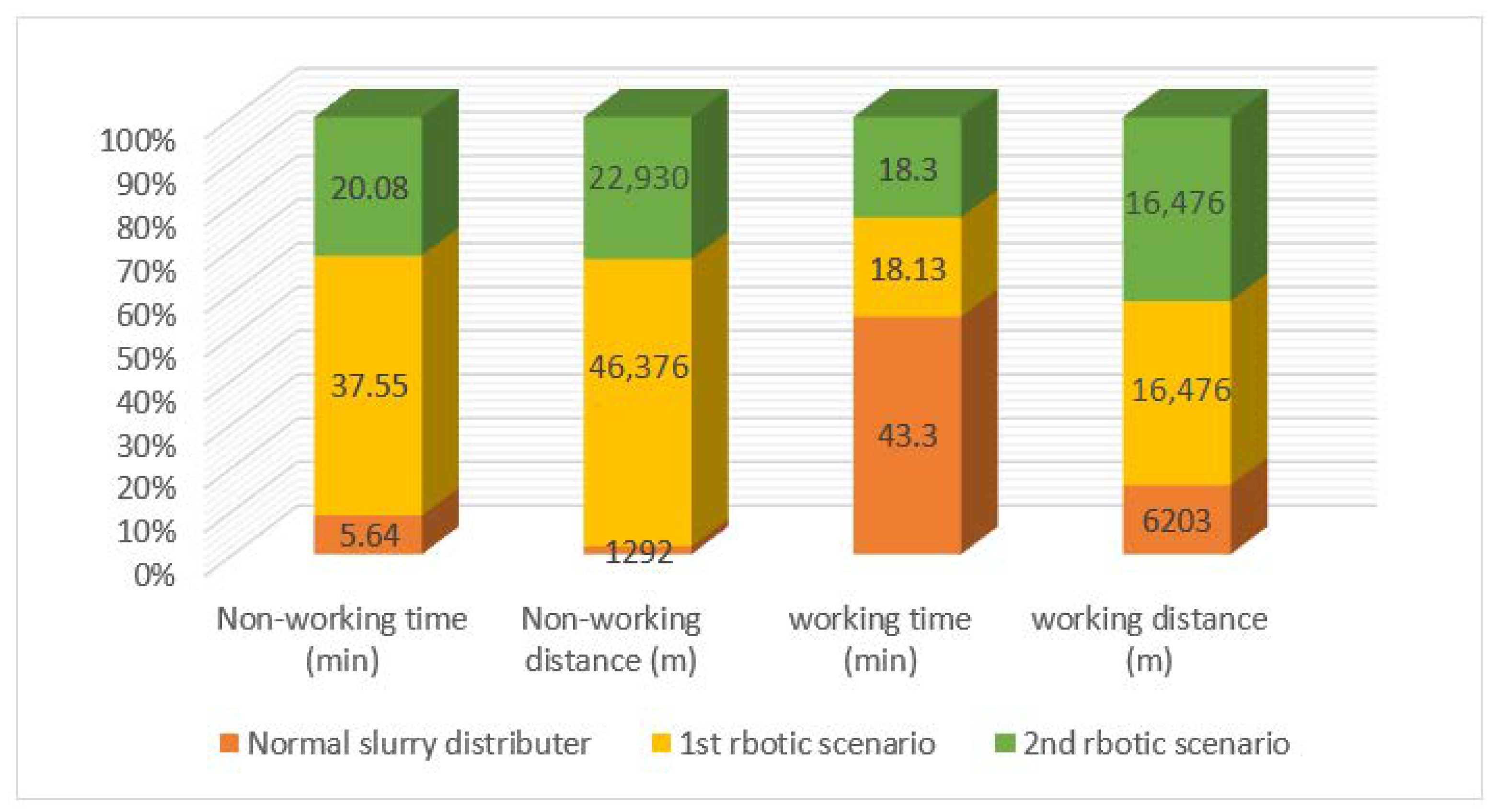
Non-working distance (meter)1292
Non-working time (minutes)5.64
Working distance (meter)6203
Working time (minutes)43.3
Table 6. The optimized field coverage plan with the results of the simulation model for the fertilizing operation by using three homogenous robots with the capacity of 0.8 m3 in the sample field (1st scenario).
Solution (1st Scenario)<1, 106, 109, 114, 117, 122, 125, 130, 133, 138, 2, 85, 90, 93, 98, 101, 142, 145, 1, 82, 77, 74, 69, 1, 150, 153, 158, 161, 166, 169, 1, 66, 61, 58, 2, 53, 50, 45, 1, 174, 177, 182, 185, 1, 42, 37, 34, 2, 29, 26, 21, 1, 18, 13, 1, 10, 5, ‘28h’, ‘29h’,…, ‘49h’, ‘50h’, 1, 3, 2, 7, 2, 11, 2, 15, 2, 19, 2, 23, 2, 27, 2, 31, 2, 35, 2, 39, 2, 43, 2, 47, 2, 51, 2, 55, 2, 59, 2, 63, 2, 67, 2, 71, 2, 75, 2, 79, 2, 83, 2, 87, 2, 91, 2, 95, 2, 99, 2, 103, 2, 107, 2, 111, 2, 115, 2, 119, 2, 123, 2, 127, 2, 131, 2, 135, 2, 139, 2, 143, 2, 147, 2, 151, 2, 155, 2, 159, 2, 163, 2, 167, 2, 171, 2, 175, 2, 179, 2, 183, 1, ‘86h’, ‘87h’,…,’128h’, ‘129h’, 2, ‘134h’, ‘135h’,…,’154h’, ‘155h’, ‘5h’, ‘6h’,…,’26h’, ‘27h’, 1, ‘130h’, ‘131h’, ‘132h’, ‘133h’, ‘51h’, ‘52h’,…,’84h’, ‘85h’, 1>
Non-Working Distance (Meter)Non-Working Time (Minutes)Working Distance
(Meter)
Working Time
(Minutes)
18,02637.55547518.13
14,09329.35553617.97
14,25729.7546517.49
46,37637.5516,47618.13
Table 7. The optimized field coverage plan with the results of the simulation model for fertilizing operation by using three homogenous robots with the capacity of 0.8 m3 in the sample field (2nd scenario).
Solution (2nd Scenario)<1, 106, 109, 114, 117, 122, 125, 130, 133, 138, 2, 85, 90, 93, 98, 101, 142, 145, 1, 82, 77, 74, 69, 1, 150, 153, 158, 161, 166, 169, 1, 66, 61, 58, 2, 53, 50, 45, 1, 174, 177, 182, 185, 1, 42, 37, 34, 2, 29, 26, 21, 1, 18, 13, 1, 10, 5, ‘28h’, ‘29h’,…, ‘49h’, ‘50h’, 1, 4, 2, 7, 1, 12, 2, 15, 1, 20, 2, 23, 1, 28, 2, 31, 1, 36, 2, 39, 1, 44, 2, 47, 1, 52, 2, 55, 1, 60, 2, 63, 1, 68, 2, 71, 1, 76, 2, 79, 1, 84, 2, 87, 1, 92, 2, 95, 1, 100, 2, 103, 1, 108, 2, 111, 1, 116, 2, 119, 1, 124, 2, 127, 1, 132, 2, 135, 1, 140, 2, 143, 1, 148, 2, 151, 1, 156, 2, 159, 1, 164, 2, 167, 1, 172, 2, 175, 1, 180, 2, 183, 1, ‘86h’, ‘87h’,…,’128h’, ‘129h’, 2, ‘134h’, ‘135h’,…,’154h’, ‘155h’, ‘5h’, ‘6h’,…,’26h’, ‘27h’, 1, ‘51h’, ‘52h’,…,’84h’, ‘85h’,‘130h’, ‘131h’, ‘132h’, ‘133h’, 2>
Non-Working Distance (Meter)Non-Working Time (Minutes)Working Distance
(Meter)
Working Time
(Minutes)
964020.08552918.3
670413.97536217.61
658613.72558517.67
22,93020.0816,47618.3
Publisher’s Note: MDPI stays neutral with regard to jurisdictional claims in published maps and institutional affiliations.

