Early Detection of Mold-Contaminated Peanuts Using Machine Learning and Deep Features Based on Optical Coherence Tomography

Abstract

Fungal infection is a pre-harvest and post-harvest crisis for farmers of peanuts. In environments with temperatures around 28 °C to 30 °C or relative humidity of approximately 90%, mold-contaminated peanuts have a considerable likelihood to be infected with Aflatoxins. Aflatoxins are known to be highly carcinogenic, posing danger to humans and livestock. In this work, we proposed a new approach for detection of mold-contaminated peanuts at an early stage. The approach employs the optical coherence tomography (OCT) imaging technique and an error-correcting output code (ECOC) based Support Vector Machine (SVM) trained on features extracted using a pre-trained Deep Convolutional Neural Network (DCNN). To this end, mold-contaminated and uncontaminated peanuts were scanned to create a data set of OCT images used for training and evaluation of the ECOC-SVM model. Results showed that the proposed approach is capable of detecting mold-contaminated peanuts with respective accuracies of approximately 85% and 96% after incubation periods of 48 and 96 h.

1. Introduction

Peanut kernels contribute to the production of essential nutrients such as proteins, fat, carbohydrates, vitamins, and inorganic salts. They are also considered to be moderately high-oil oilseed and the oil from peanuts is regarded as a premier frying oil worldwide. This is because it is stable at high temperatures and has a higher smoke point than other edible oils [1]. Furthermore, peanuts also play a role in the manufacturing of ready-to-use therapeutic food treatment for malnutrition diseases such as kwashiorkor in some countries [2]. Nonetheless, the composition of peanuts provides an excellent environment for the growth of fungi and for toxin productions given the suitable humidity and temperature conditions during both pre-harvest and post-harvest [1,3,4].

Elevated temperatures and insect activity are significant factors for pre-harvest contamination. As for post-harvest, warm temperatures and high humidity are the most contributing factors. According to the International Agency for Research on Cancer of the World Health Organization, Aflatoxins are deemed as Class 1 human carcinogens. They are also known to be mutagenic, hepatotoxic, and teratogenic [5]. Exposure to aflatoxins is known to cause both chronic and acute hepatocellular injuries. In April 2004, one of the largest aflatoxin outbreaks occurred in rural Kenya, resulting in 317 cases and 125 deaths [6]. Later, in 2012, the Centers for Disease Control and Prevention (CDC) estimated a world population of more than $4.5$ billion people is exposed to aflatoxins. Moreover, fungal and aflatoxin contamination of crops has also resulted in some drastic economic losses in the past [7]. Considering that high temperature and high humidity are a natural phenomenon which occurs consistently, it is crucial to develop methods to detect the presence of mold in peanuts. When fungal growth is detected at an early stage, it will considerably reduce the chances of exposure to Aflatoxins.

Up to this day, several methods have been developed and used to determine the presence of aflatoxins in peanuts. Most of these methods are mainly chromatographic [8]. These include thin-layer chromatography (TLC), gas chromatography (GC), and high-performance liquid chromatography (HPLC) [9,10,11,12]. Although these techniques are very sensitive and can detect the presence of Aflatoxins with great accuracy, they rely heavily on a lot of expensive laboratory equipment to identify the genus and morphological characterization, including macroscopic and microscopic characteristics of the fungus. Moreover, they are time-consuming, require experienced personnel and a well-equipped laboratory. Additionally, they are destructive to samples, rendering them unsuitable for use in in-line food sorting and production systems [13].

The other category of methods is optical-based. It uses imaging or spectroscopic techniques such as fluorescence spectroscopy (FS), near infrared (NIR) spectroscopy, and hyperspectral imaging systems (HSI) [4,14,15]. Promising results have been achieved by using these optical techniques. FS-based optical methods operate on the principle that when contaminated food is exposed to UV light, the fluorescence phenomenon occurs. This makes it possible to detect aflatoxin contamination using fluorescence characteristics [16]. However, the use of fluorescence spectra in agricultural products has been noted as difficult due to the complexity of background food matrices [13]. This is because background food contains a great variety of natural fluorescent compounds that can overlap with the analyte signal. When food is irradiated by a continuous fluctuating frequency of the NIR light, it emits a different wavelength of light. Henceforth, causing molecular vibrations, specifically the overtones and combination of fundamental vibrations. Since the chemical bonds between light atoms in Aflatoxins have high vibrational frequencies, the overtones and combination bands are detectable in the NIR region [16]. Besides being non-invasive, there is usually no need for sample preparations. Therefore, the analysis is simple and fast [17]. However, the NIR spectra are generally complex due to highly overlapping bands and weak absorption bands associated with overtones and combinations of vibrational bonds [18]. Moreover, the use of these techniques usually requires a substantial number of spectral treatments before sophisticated methods are defined [19].

Over the past few years, a considerable number of studies has been started exploiting the HSI technique. HSI technique integrates NIR spectroscopy and imaging techniques with an aim to simultaneously provide both spectral and spatial information of the specimen being analyzed. The images acquired using HSI consist of two spatial dimensions and one spectral dimension made up of hundreds of continuous wavebands for each spatial pixel of the specimen. Henceforth, compared to the conventional spectroscopic techniques, the added spatial dimension enables mapping of chemical components in peanuts, making it easy to detect fungal infections and aflatoxin contamination [20,21,22]. However, this technique also inherits the challenges that are presented by the FS-based and NIR-based approaches.

In this work, we are presenting a new optical-based technique for the detection of mold-contaminated peanut kernels utilizing Optical Coherence Tomography (OCT) images. OCT imaging technique generates, micrometer-resolution, 2D and 3D images from within optical scattering media. It is non-invasive, non-destructive and capable of generating real-time high-resolution tomographic images. Moreover, OCT has been fundamentally applied in a wide range of applications, such as early detection of cancer [23], ophthalmology [24], dermatology [25], and art conservation [26]. In addition, OCT has also been employed in several agricultural applications such as quality assessment of leaf samples [27,28], monitoring seed growth [29] and identification of defects and diseases in seeds [30,31]. These studies and several other have shown the usefulness of OCT in agricultural studies to be prominent. With the OCT imaging technique, we were able to capture images showing the top layers of peanut kernels without destroying the samples. This allowed us to extract features from the internal structures of the peanuts using simple feature extraction methods. Therefore, removing the complexity presented by these state of the art methods.

In most computer vision applications, the type of features and the process of feature extraction are crucial. Recent studies have shown to favor the use of convolutional neural networks (CNN) to solve OCT image classification problems [32,33,34,35]. On that note, in this study we determined the performance of deep features extracted OCT images using a pre-trained deep CNN on mold contaminated peanuts. We compared the performance of this method against the conventional Speeded Up Robust Features (SURF), Histogram of Oriented Gradients (HOG), KAZE, and Maximally Stable Extremal Regions (MSER) features [36,37,38,39,40]. Our objectives were to:

• Find suitable features for representing the OCT images extracted from peanuts,
• Identify a suitable classification models and feature combinations for the task detecting the mold-contaminated peanuts by evaluating the performance of those methods on our data set,
• Evaluate accuracy proposed method against the contamination period.

2. Materials and Methods

2.1. Experiments and OCT Image Dataset

2.1.1. Preparing the Spore Suspension

Aspergillus flavus (AS3.3950, Shanghai Luwei Technology Co. Ltd., Shanghai, China) mold strain was plated on potato dextrose agar medium (PDA) and then incubated in the dark at 30 °C and $90\%$ relative humidity (RH) for seven days in order to produce significant sporulation [41]. Afterward, the spores were suspended in 10 mL of the sterile aqueous 0.05 mL/mL of Tween 80, followed by gently rubbing the surface of the mold plate using the sterilized L-shaped glass rod [42]. The formed suspension was then filtered through a 2-layered cheesecloth. Finally, the pour plate method was used to estimate the concentration of the spore suspension. The spore suspension was kept in a refrigerated environment with temperatures around 1 °C to 4 °C until use [19].

2.1.2. Peanut Sampling and Inoculation

Two kilograms of peanut kernels was purchased from four local vendors in Hangzhou, Zhejiang province, China and used as the original sample. Afterward, three groups of mold-uncontaminated peanuts were hand selected from the original sample.

Each group contained 20 peanut kernels. The spore suspension with a concentration of $1.88\times {10}^6$ colony forming units per milliliter, CFU mL${}^{-1}$ was used to inoculate one of the three groups by soaking the peanut kernels in 10 mL of the spore suspension for three minutes. The peanut kernels were dried by placing them between two layers of Sterile paper. Of the remaining two groups, one was soaked in the $70\%$ ethanol for two minutes, sufficient to kill fungi, yeasts, and bacteria on the surface of the peanut kernels [43]. Sterile paper was then used to dry the peanuts kernels. This was then used as the control group in the experiment. To simulate the natural growth of mold on the peanut kernels, the third sample was neither sterilized with ethanol nor inoculated with the spore suspension. It was put in a PDA plate to provide a conducive environment for the mold to grow [44]. Lastly, for all the peanut kernels in the three groups (experimental group A, control group and experimental group B, respectively), a region of interest (ROI) (≈5 mm in diameter) was marked and 5 scans were acquired by randomly scanning inside the ROI using an OQ Labscope $2.0$ (Lumedica, Durham, North Carolina, US) system with a wavelength of 840 nm. Afterward, the three samples were then incubated at 30 °C and $90\%$ relative humidity to provide the condition favorable for the growth of Aspergillus flavus [3,4,44,45,46].

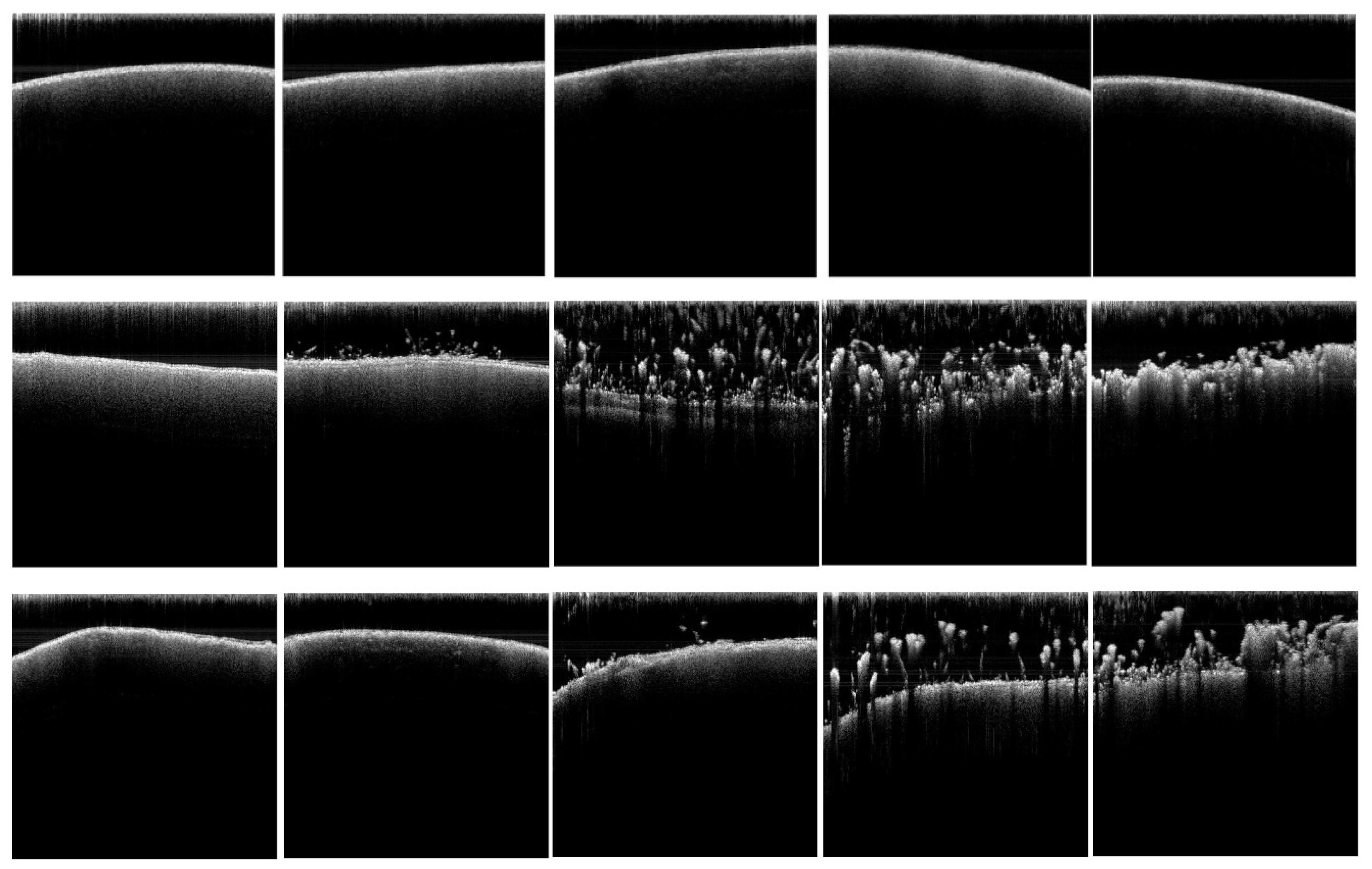
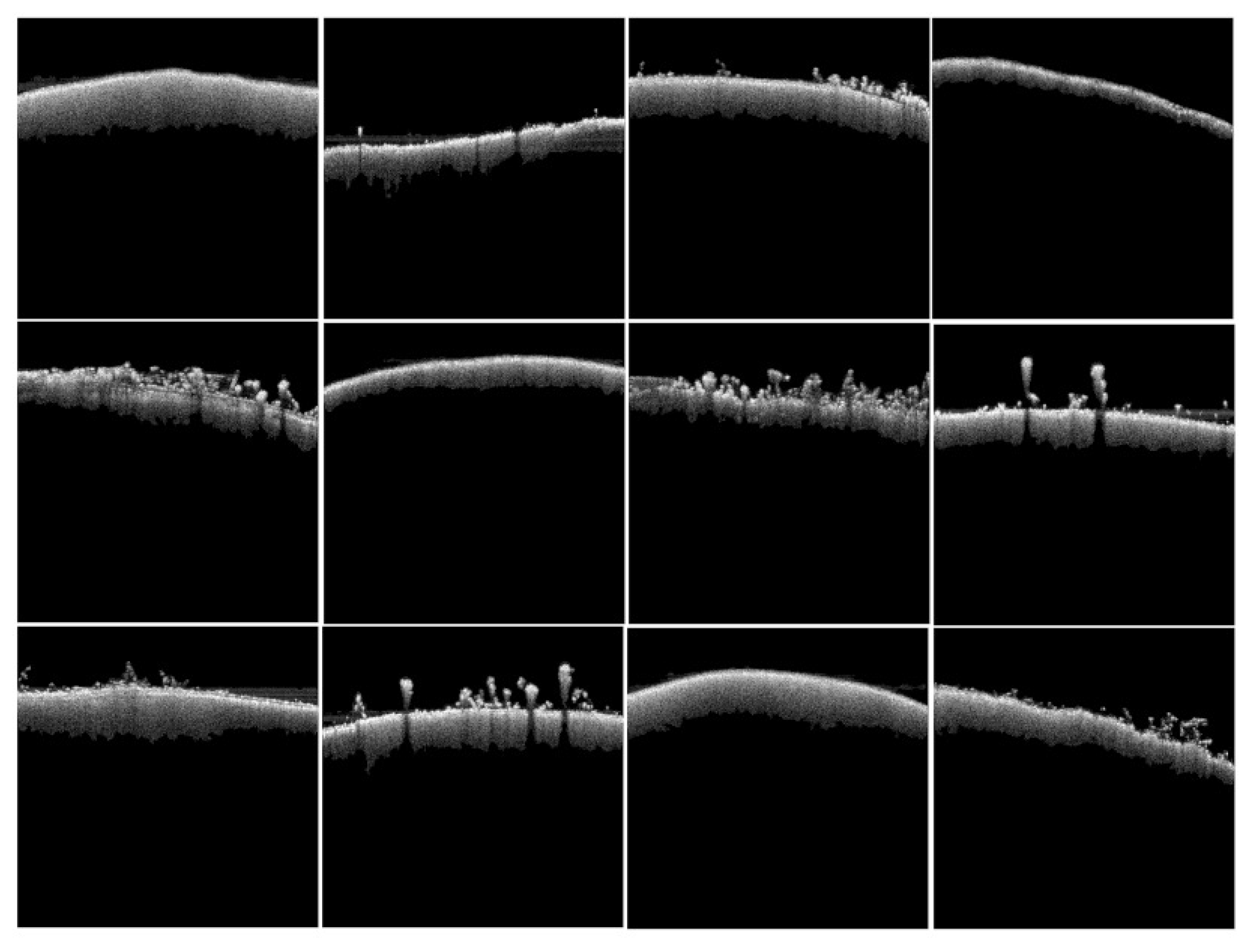
2.1.3. Optical Coherence Tomography Images Dataset

The optical coherence tomographic imaging technique generates micrometer-resolution 2D and 3D images from within optical scattering media. This technique has a lot of applications in the medical field, because of its ability to provide non-invasive diagnostic images [47]. This allows our method to detect mold-contaminated peanut kernels without destroying the peanut samples.

After every 24 h, we used the OQ Labscope $2.0$ (Lumedica, Durham, NC, USA) system to scan the incubated peanut kernels in the control group, experimental group A, and experimental group B. Each scan consisted of thirty, 2-dimensional, $512\times 512$ pixels OCT images plus one generated $512\times 512$ pixels average OCT image. The experiment lasted for 96 h which resulted in a data set with a total of 46,500 OCT images. We later used this data set to train and evaluate the performance of the proposed ECOC-SVM and K-Nearest Neighbors (KNN) classification models.

Figure 1 shows OCT images of three exemplar peanut kernels from the respective control group, the experimental group A, and the experimental group B. We used the OCT images of the peanuts in the control group, and the experimental group A, as the training data set. Lastly, we created a test data set with the OCT images from experimental group B.

2.2. Proposed Method

When combined, Figure 2 and Figure 3 shows our framework for the early detection of mold-contaminated peanut kernels. The framework is split into two phases (shown respectively, in Figure 2 and Figure 3). We tasked the first phase with the training of the ECOC-SVM classification model employed in the second phase.

Given the labeled training OCT images from our training data set, the first step in this phase is noise reduction. We reduce the noise in OCT input images before passing them through our feature descriptor. The descriptor uses a DCNN trained on a large-scale data set to extract the deep features from the OCT images. Finally, we use these features to train the ECOC-based SVM classification model.

The second phase uses the trained model to classify the OCT images of the peanut kernels. Before the classification of new images, we utilize the same noise reduction and deep feature extraction processes used in phase one.

The following subsections will give a breakdown of the main processes we used in the framework.

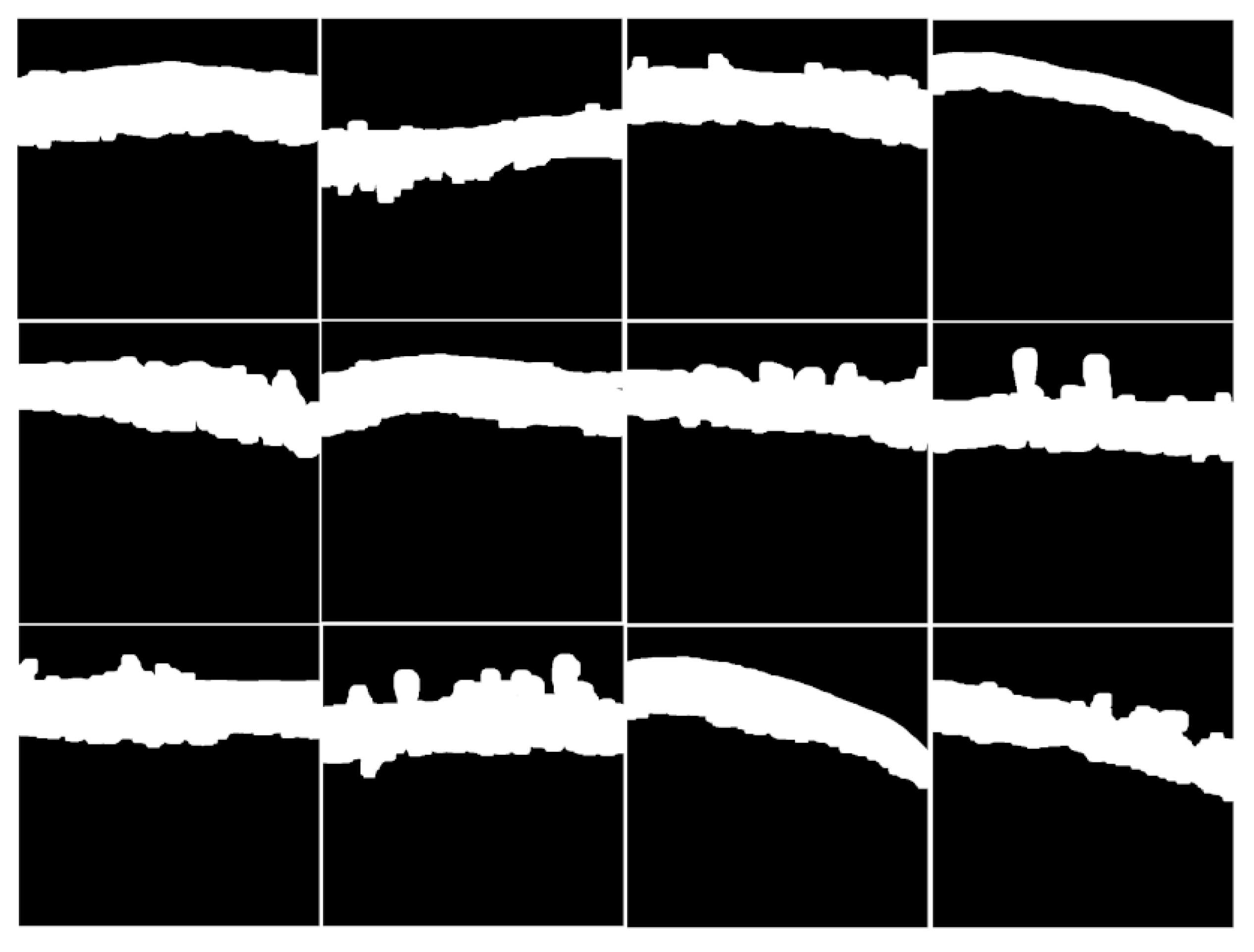
2.2.1. Noise Reduction and OCT Image Background Removal

OCT images are prone to the coherent noise, which is the speckle noise. This degrades the contrast and the detail structural information of the OCT image, thus imposing significant limitations on the classification capability of our method. Therefore, prior to deep-feature extraction we pass all the images through a $10\times 10$ median filter. Next, the filtered images are binarized using Otsu’s method [48] and then the largest connected components are extracted to generate a binary mask. The edges of the generated mask are smoothened by a $20\times 20$ average filter to make sure that the mask includes as much area of the connected component as possible. Finally, we multiply the original average of the OCT images with the mask, producing an OCT image with all the background, non-peanut, and non-mold pixels replaced with the value zero.

Figure 4, Figure 5 and Figure 6 shows the input, intermediated results of the OCT image pre-processing, as well as the final segmented image.

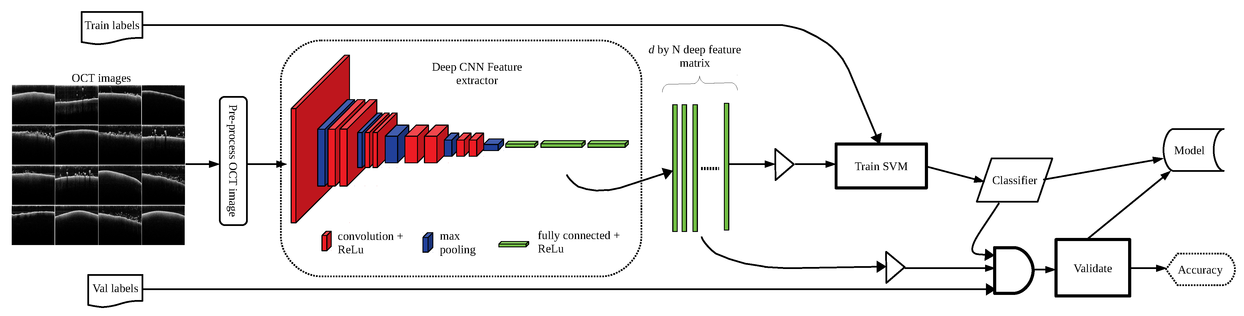
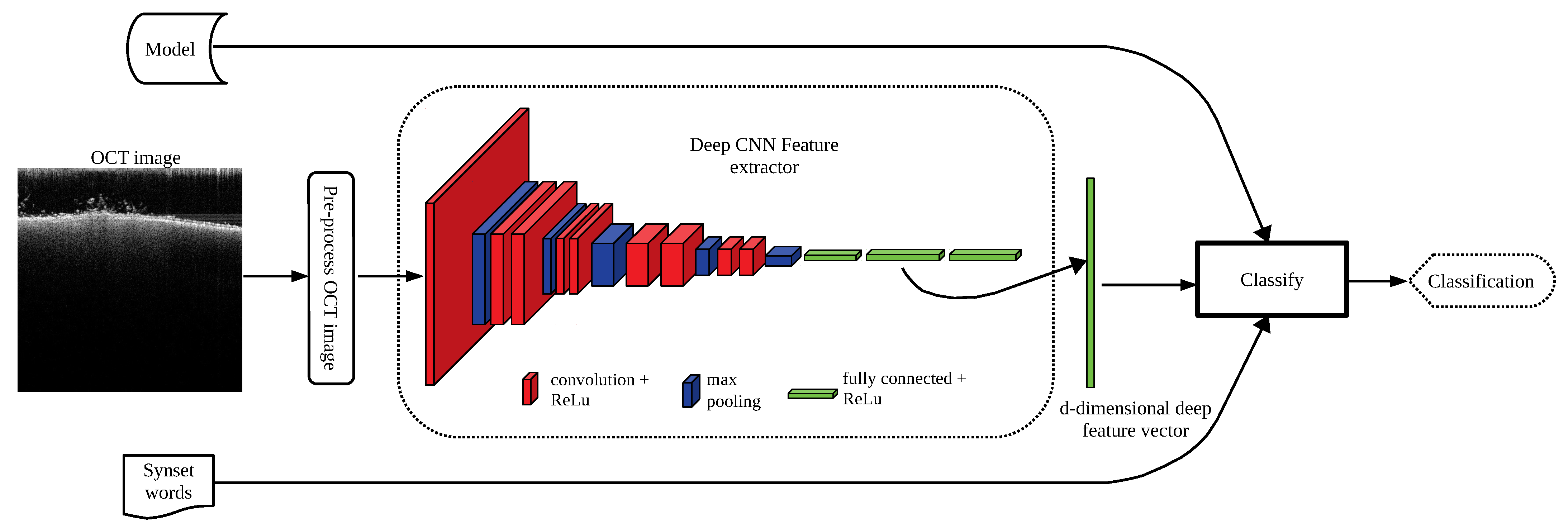
2.2.2. Deep Feature Extraction and ECOC-SVM Model Training

Advancements in the efficiency of DCNNs have resulted in the use of deep features extracted from the high-level layers of the DCNNs, mainly the fully connected layers. These features have proven to be very effective with state of the art performance on a variety of image datasets [49,50]. However, the effectiveness of these features depended largely on the size of the data set used to train the CNN model [49,51,52]. Considering the size limitations of our final training database and the scarcity of large-scale datasets of OCT images, we used Visual Geometry Group’s (VGG), VGG 16 DCNN model trained on the ILSVRC 2015 benchmark data set in our feature descriptor. This DCNN produced promising results on several methods when used on OCT images [33,34,35]. Mathematical explanation for the process of extracting deep features from a CNN was provided in [53].

Our feature descriptor harvests the responses from one of the VGG 16 DCNN model’s high-level fully-connected layers, fc6 [54]. Finally, we use the $1\times 4096$ deep-feature vector representations of the OCT images from the descriptor to train the ECOC-SVM classification model.

3. Results and Discussion

In this section, we evaluate the performance of the ECOC-SVM classification models trained on Deep, SURF, KAZE, MSER, and HOG features for the early detection of mold-contaminated peanuts using performance metrics for evaluating classification methods. We also show the performance results for KNN-based classification models that we trained, tested, and evaluated by the same performance metrics.

From our observations during the incubation and the acquisition of OCT images, the peanuts in the control group remained uncontaminated for the entire 96 h. As for the experimental group B, the mold became visible on most of the peanuts after a period of 72 h. Lastly, we started to observe mold on some of the peanuts in experimental group A after a period of 24 h. The same differences between mold-contaminated and mold-uncontaminated peanut kernels can be noticed evidently in the OCT images displayed in Figure 1. For the exemplar kernels shown in the third row of Figure 1, this difference starts to show in the scan taken after 48 h and after 24 h for the second row.

With negative labels assigned to OCT images of mold-uncontaminated peanuts and the positive labels assigned to the OCT images mold-contaminated peanuts, seven-eighths of the training data set was used to train the ECOC-SVM and the supplementary KNN classification models. The remainder of the training data set was used as a validation data set to evaluate the classification model at the training phase. Afterward, we used the 500 average OCT images in our test data set to evaluate the performance of the classification models on peanuts contaminated from naturally grown mold.

All methods were implemented using the MATLAB 2018a (Mathworks, Natick, MA, USA) and were run on a computer with an 8 GB RAM, 1 TB HDD, 128 GB SSD and equipped with an NVIDIA GeForce GTX 960.

Table 1. The precision, recall, f1-score, accuracy, and balanced accuracy of the proposed and evaluation methods on the training data set. The precision, recall, f1-score, accuracy, and balanced accuracy values range from 0 to 1 inclusive.

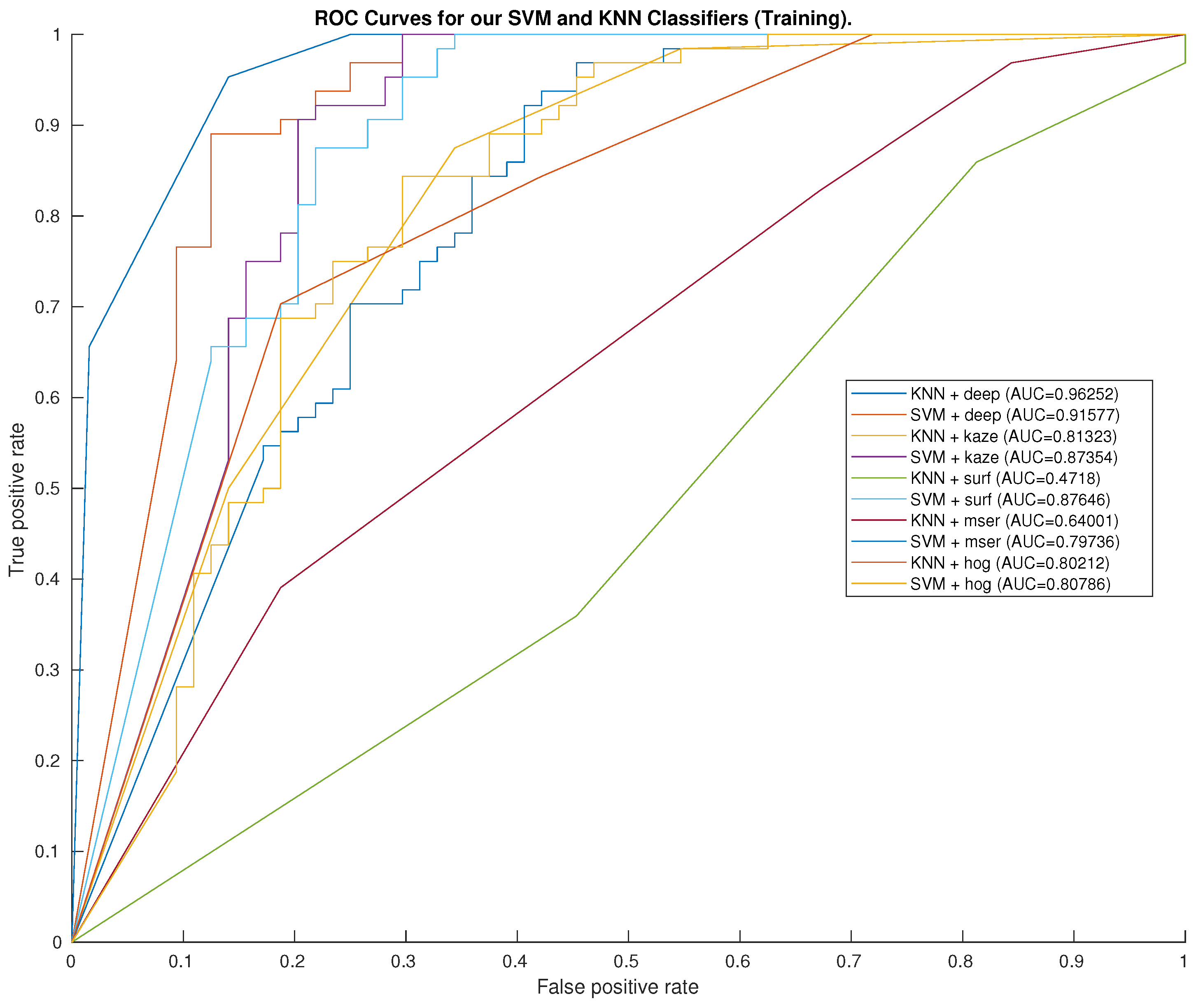
Method	Precision	Recall	F1-Score	Accuracy	Balanced Accuracy
KNN + Deep features	0.95	0.86	0.90	0.91	0.91
ECOC-SVM + Deep features	0.92	0.77	0.84	0.85	0.85
ECOC-SVM + KAZE features	0.94	0.72	0.81	0.84	0.84
ECOC-SVM + SURF features	0.92	0.70	0.80	0.82	0.82
KNN + KAZE features	0.84	0.66	0.74	0.77	0.77
ECOC-SVM + HOG features	0.75	0.70	0.73	0.73	0.73
ECOC-SVM + MSER features	0.81	0.59	0.68	0.73	0.73
KNN + HOG features	0.79	0.58	0.67	0.71	0.71
KNN + MSER features	0.66	0.33	0.44	0.58	0.58
KNN + SURF features	0.57	0.19	0.28	0.52	0.52

and

Table 2. The precision, recall, f1-score, accuracy, and balanced accuracy of the proposed and evaluation methods on the test data set. The precision, recall, f1-score, accuracy, and balanced accuracy values range from 0 to 1 inclusive.

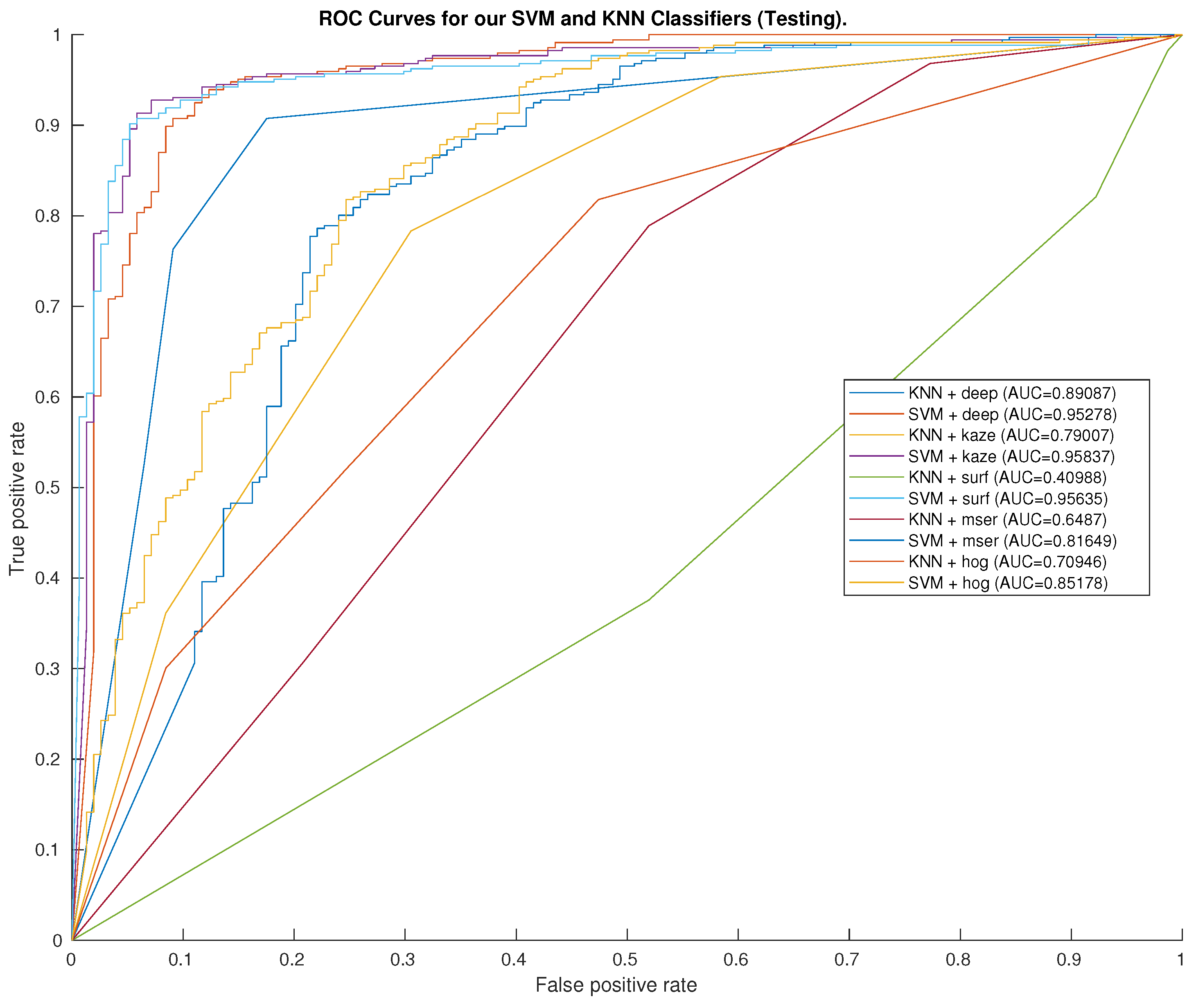
Method	Precision	Recall	F1-Score	Accuracy	Balanced Accuracy
ECOC-SVM + Deep features	0.76	0.92	0.83	0.89	0.89
ECOC-SVM + SURF features	0.73	0.97	0.83	0.88	0.90
ECOC-SVM + KAZE features	0.70	0.95	0.81	0.86	0.89
KNN + Deep features	0.63	0.91	0.74	0.81	0.84
ECOC-SVM + MSER features	0.74	0.74	0.68	0.79	0.78
KNN + KAZE features	0.59	0.70	0.64	0.76	0.74
KNN + MSER features	0.50	0.48	0.49	0.69	0.63
ECOC-SVM + HOG features	0.48	0.88	0.62	0.67	0.73
KNN + HOG features	0.41	0.75	0.53	0.59	0.63
KNN + SURF features	0.16	0.08	0.11	0.59	0.45

show the precision, recall, F1 Score, and accuracy values for all the implemented classifiers on training and testing datasets, respectively. We also included the balanced accuracy to give a comprehensive evaluation.

The KNN model trained on deep features outperformed the other methods on the training data set. It achieved an accuracy of approximately $91\%$. The ECOC-SVM model trained on deep features followed with an approximate accuracy of $85\%$. In general, KNN classification models can achieve great performance on data that closely resembles that was used to KNN classification model. Henceforth, this and the use of deep features can explain the spectacular performance of the KNN model trained on deep features. ECOC-SVM classifiers trained on KAZE and SURF features similarly managed to achieve good accuracy on the training data set. Both of the models trained on HOG features managed to achieve accuracy within the range of $70\%\to 75\%$. Lastly, both of the models trained on MSER features performed poorly. Herein, the superiority of deep features extracted from the OCT images was evident in the performance of the classification models that we trained using these features.

Figure 7 and Figure 8 display the Receiver Operating Characteristic (ROC) curves for all the methods along with the corresponding Area Under the Curve (AUC). Although the use of AUC has been challenged due to some of its problems [55,56,57], in this work, we employed it to aid with the performance evaluation of the implemented classification models [58]. The curves in Figure 7 also resemble similar traits as the findings shown in Table 1. In this case, the models trained on deep features had significant AUC values as compared to the rest of the models trained on the other features.

The results obtained on the test data set produces a slightly different trend. The ECOC-SVM models trained on Deep, SURF, and KAZE features achieved good accuracies with a slight deviation from the accuracy values on the training data set. On the other hand, the KNN model trained on the deep features had an accuracy decrease of approximately $10\%$. The rest of the methods had accuracies varying from $59\%\to 79\%$. The AUC values of the ROC curves in Figure 8 also support the aforementioned analysis. Furthermore, we evaluated the four models on small sets of the test data set. These sets comprised of the average OCT images of moldy peanut kernels at various stages of contamination.

Table 3. The accuracy results against incubation time for the best four methods on the test data set. The incubation period starts from 0 h with increments of 24 h until 96 h. Accuracy values range from 0 to 1 inclusive.

Method	0 h	24 h	48 h	72 h	96 h
ECOC-SVM + Deep features	0.91	0.92	0.90	0.74	0.96
ECOC-SVM + SURF features	0.92	0.91	0.89	0.72	0.95
ECOC-SVM + KAZE features	0.90	0.91	0.89	0.68	0.92
KNN + Deep features	0.78	0.85	0.82	0.68	0.91

shows the accuracy results for this analysis.

The ECOC-SVM models performed better as compared to the KNN model. From this analysis, we can see the differences in performance (AUC, F1-Score, accuracy, and the balanced accuracy) of the trained models over the training and the testing data from the results shown in Table 1 and Table 2.

Table 4. The differences in AUC, F1-Score, accuracy, and the balanced accuracy as a percentage of the top four methods on the training data set and the test data set. The differences of AUC, F1-Score, accuracy, and the balanced accuracy are respectively denoted by ${\delta }_{auc}$, ${\delta }_{f1}$, ${\delta }_{accu}$, and ${\delta }_{b-accu}$.

Method	${\mathit{\delta }}_{\mathbf{auc}}(\%)$	${\mathit{\delta }}_{\mathit{f}1}(\%)$	${\mathit{\delta }}_{\mathbf{accu}}(\%)$	${\mathit{\delta }}_{\mathit{b}-\mathbf{accu}}(\%)$
ECOC-SVM + Deep features	3.7	0.48	3.44	3.44
ECOC-SVM + SURF features	7.99	3.36	5.77	8.25
ECOC-SVM + KAZE features	8.48	0.65	2.41	5.03
KNN + Deep features	7.17	15.69	9.82	7.02

shows the differences of the top 4 classification models. We denoted the values by ${\delta }_{auc}$, ${\delta }_{f1}$, ${\delta }_{accu}$, and ${\delta }_{b-accu}$. The deltas were calculated using Equation (1).

$${\delta }_x=(x_{train}-x_{test})\times 100$$

(1)

where ${\delta }_x$ is the percentage difference for the performance metric x obtained on the training data set and the test data set.

When evaluated on new data (test data set) different from that used during the training phase, the ECOC-SVM models trained on Deep, SURF, and KAZE features achieved better accuracies with a slight deviation from the accuracy values on the training data set. On the other hand, the performance of the KNN model trained on deep features dropped significantly. In general, this can be attributed to the learning approaches of the two classification algorithms as well as the type of features used to train the models.

The ECOC-SVM model trained on deep features demonstrated promising and fairly consistent performance than the others on detecting the moldy peanut kernels at different phases of contamination. It achieved an average accuracy of approximately $89\%$ with its outstanding accuracy of $96\%$ at the scans procured after 96 h. These results indicate that the proposed method can achieve early mold detection on peanuts with satisfactory accuracy.

Despite the lack of studies mainly focusing on mold-contamination detection of peanuts using OCT images, we were still able to compare these results with those achieved by some of the current optical-based methods for detecting mold-contaminated peanuts. The work in [43] applied the visible-near infrared (Vis-NIR) together with Partial Least Squares Discriminate Analysis (PLS-DA). The PLS-DA produced overall accuracies ranging from $88\%\to 95\%$ using the full Vis-NIR spectra. Afterwards, the research in [21] employed Wavelet transformations and HSI techniques to identify moldy peanut kernels. In addition to using the PLS-DA, they also used the traditional SVM classification model. The outcome indicated that uncontaminated and contaminated peanuts can be separated with an accuracy of at least approximately $96\%$ [21].

Generally, the results from these methods mainly focused on the whole contamination procedure. However, we can still compare the overall accuracy achieved by our method to that of the state of the art methods. Notwithstanding the differences in systems, optical imaging technologies, features, and samples, our method still managed to detect mold-contaminated peanut kernels with accuracies within the same range as the state of the art methods mentioned above. Moreover, our method achieved good performance without the need for complex procedures required by some of these methods. Additionally, our study proposed an end-to-end framework that is quick to set up, easier to use, and does not require complex algorithms.

The use of OCT images allows deep features from the peanuts’ sub-surface to be used in training the ECOC-SVM classifier. This entails that the trained classifier will be capable of classifying OCT images down to the peanut’s sub-surface level. The addition of deep features representing the tissue morphology of peanut kernels allows our method to detect sub-surface mold contamination.

4. Conclusions

This work introduced a new optical-based, non-invasive, and non-destructive classification framework for early detection of mold-contaminated peanut kernels during post-harvest. Out of all the variations of the classification models trained and tested, the ECOC-SVM classification model trained on deep features extracted from OCT images of peanut kernels showed promising and reliable results. It managed to detect moldy peanuts with good accuracy of approximately $85\%$ and $89\%$ on both the training and testing datasets, respectively. It also achieved an average time-based accuracy of $89\%$, with its highest accuracy of $96\%$ at the scans acquired after 96 h.

In the future, we need to assess the upshot of introducing a filtering algorithm to reduce the speckle noise in the segmented images used to train the classifier. Furthermore, having a larger OCT image data set of peanut kernels will allow us to evaluate the performance of an end-to-end CNN for mold-contaminated and mold-uncontaminated peanut kernels classification. Additionally, the preference of ECOC-SVM over the traditional SVM classifier will enable us to examine the age of the detected mold [59].

The proposed technique could also detect or classify other crops prone to mold contamination, such as maize, rice, etc. We can easily accomplish this by training the ECOC-SVM on VGG16 deep features or SURF features extracted from the OCT images of the respective crops.

References

- List, G.R. Processing and food uses of peanut oil and protein. In Peanuts; Elsevier: Amsterdam, The Netherlands, 2016; pp. 405–428. [Google Scholar]
- Ali, E.; Zachariah, R.; Dahmane, A.; Van den Boogaard, W.; Shams, Z.; Akter, T.; Alders, P.; Manzi, M.; Allaouna, M.; Draguez, B.; et al. Peanut-based ready-to-use therapeutic food: Acceptability among malnourished children and community workers in Bangladesh. Public Health Action 2013, 3, 128–135. [Google Scholar] [CrossRef] [Green Version]
- Okoth, S.; De Boevre, M.; Vidal, A.; Diana Di Mavungu, J.; Landschoot, S.; Kyallo, M.; Njuguna, J.; Harvey, J.; De Saeger, S. Genetic and toxigenic variability within Aspergillus flavus population isolated from maize in two diverse environments in Kenya. Front. Microbiol. 2018, 9, 57. [Google Scholar] [CrossRef] [PubMed]
- Wu, Q.; Xu, H. Design and development of an on-line fluorescence spectroscopy system for detection of aflatoxin in pistachio nuts. Postharvest Biol. Technol. 2020, 159, 111016. [Google Scholar] [CrossRef]
- Omotayo, O.P.; Omotayo, A.O.; Mwanza, M.; Babalola, O.O. Prevalence of mycotoxins and their consequences on human health. Toxicol. Res. 2019, 35, 1–7. [Google Scholar] [CrossRef] [Green Version]
- Centers for Disease Control and Prevention. Outbreak of aflatoxin poisoning-eastern and central provinces, Kenya, January–July 2004. MMWR. Morb. Mortal. Wkly. Rep. 2004, 53, 790. [Google Scholar]
- Vardon, P.; McLaughlin, C.; Nardinelli, C. Potential Economic Costs of Mycotoxins in the United States; Council for Agricultural Science and Technology Task Force Report; Council for Agricultural Science and Technology: Ames, IA, USA, 2003. [Google Scholar]
- Cheng, Z.; Wacoo, A.P.; Wendiro, D.; Vuzi, P.C.; Hawumba, J.F. Methods for Detection of Aflatoxins in Agricultural Food Crops. J. Appl. Chem. 2014, 2014, 706291. [Google Scholar] [CrossRef] [Green Version]
- Herzallah, S.M. Determination of aflatoxins in eggs, milk, meat and meat products using HPLC fluorescent and UV detectors. Food Chem. 2009, 114, 1141–1146. [Google Scholar] [CrossRef]
- Wang, W.; Heitschmidt, G.W.; Ni, X.; Windham, W.R.; Hawkins, S.; Chu, X. Identification of aflatoxin B1 on maize kernel surfaces using hyperspectral imaging. Food Control 2014, 42, 78–86. [Google Scholar] [CrossRef]
- Lavine, B.K.; Mirjankar, N.; LeBouf, R.; Rossner, A. Prediction of mold contamination from microbial volatile organic compound profiles using solid phase microextraction and gas chromatography/mass spectrometry. Microchem. J. 2012, 103, 37–41. [Google Scholar] [CrossRef]
- Lin, H.; Cousin, M. Detection of mold in processed foods by high performance liquid chromatography. J. Food Prot. 1985, 48, 671–678. [Google Scholar] [CrossRef]
- Tao, F.; Yao, H.; Hruska, Z.; Burger, L.W.; Rajasekaran, K.; Bhatnagar, D. Recent development of optical methods in rapid and non-destructive detection of aflatoxin and fungal contamination in agricultural products. TrAC Trends Anal. Chem. 2018, 100, 65–81. [Google Scholar] [CrossRef]
- Fernández-Ibañez, V.; Soldado, A.; Martínez-Fernández, A.; De la Roza-Delgado, B. Application of near infrared spectroscopy for rapid detection of aflatoxin B1 in maize and barley as analytical quality assessment. Food Chem. 2009, 113, 629–634. [Google Scholar] [CrossRef]
- Wang, W.; Lawrence, K.C.; Ni, X.; Yoon, S.C.; Heitschmidt, G.W.; Feldner, P. Near-infrared hyperspectral imaging for detecting Aflatoxin B1 of maize kernels. Food Control 2015, 51, 347–355. [Google Scholar] [CrossRef]
- Lunadei, L.; Ruiz-Garcia, L.; Bodria, L.; Guidetti, R. Image-based screening for the identification of bright greenish yellow fluorescence on pistachio nuts and cashews. Food Bioprocess Technol. 2013, 6, 1261–1268. [Google Scholar] [CrossRef]
- Osborne, B.G. Near-Infrared Spectroscopy in Food Analysis. In Encyclopedia of Analytical Chemistry; American Cancer Society: Atlanta, GA, USA, 2006. [Google Scholar] [CrossRef]
- Li, Z.; Tang, X.; Shen, Z.; Yang, K.; Zhao, L.; Li, Y. Comprehensive comparison of multiple quantitative near-infrared spectroscopy models for Aspergillus flavus contamination detection in peanut. J. Sci. Food Agric. 2019, 99, 5671–5679. [Google Scholar] [CrossRef]
- Gu, S.; Wang, J.; Wang, Y. Early discrimination and growth tracking of Aspergillus spp. contamination in rice kernels using electronic nose. Food Chem. 2019, 292, 325–335. [Google Scholar] [CrossRef]
- Jiang, J.; Qiao, X.; He, R. Use of Near-Infrared hyperspectral images to identify moldy peanuts. J. Food Eng. 2016, 169, 284–290. [Google Scholar] [CrossRef]
- Qi, X.; Jiang, J.; Cui, X.; Yuan, D. Moldy Peanut Kernel Identification Using Wavelet Spectral Features Extracted from Hyperspectral Images. Food Anal. Methods 2020, 13, 445–456. [Google Scholar] [CrossRef]
- Qiao, X.; Jiang, J.; Qi, X.; Guo, H.; Yuan, D. Utilization of spectral-spatial characteristics in shortwave infrared hyperspectral images to classify and identify fungi-contaminated peanuts. Food Chem. 2017, 220, 393–399. [Google Scholar] [CrossRef] [PubMed]
- Nandy, S.; Sanders, M.; Zhu, Q. Classification and analysis of human ovarian tissue using full field optical coherence tomography. Biomed. Opt. Express 2016, 7, 5182–5187. [Google Scholar] [CrossRef] [Green Version]
- Hu, J. Contrast Agents for Cardiovascular Optical Imaging at Molecular Level. Ph.D. Thesis, Universidad Autonoma de Madrid, Madrid, Spain, 2018. [Google Scholar]
- Pagnoni, A.; Knuettel, A.; Welker, P.; Rist, M.; Stoudemayer, T.; Kolbe, L.; Sadiq, I.; Kligman, A.M. Optical coherence tomography in dermatology. Ski. Res. Technol. 1999, 5, 83–87. [Google Scholar] [CrossRef]
- Bezerra, H.G.; Costa, M.A.; Guagliumi, G.; Rollins, A.M.; Simon, D.I. Intracoronary optical coherence tomography: A comprehensive review: Clinical and research applications. JACC Cardiovasc. Interv. 2009, 2, 1035–1046. [Google Scholar] [CrossRef] [Green Version]
- Anna, T.; Chakraborty, S.; Cheng, C.Y.; Srivastava, V.; Chiou, A.; Kuo, W.C. Elucidation of microstructural changes in leaves during senescence using spectral domain optical coherence tomography. Sci. Rep. 2019, 9, 1167. [Google Scholar] [CrossRef] [PubMed] [Green Version]
- Wijesinghe, R.E.; Lee, S.Y.; Ravichandran, N.K.; Han, S.; Jeong, H.; Han, Y.; Jung, H.Y.; Kim, P.; Jeon, M.; Kim, J. Optical coherence tomography-integrated, wearable (backpack-type), compact diagnostic imaging modality for in situ leaf quality assessment. Appl. Opt. 2017, 56, D108–D114. [Google Scholar] [CrossRef]
- Ravichandran, N.K.; Wijesinghe, R.E.; Lee, S.Y.; Shirazi, M.F.; Jung, H.Y.; Jeon, M.; Kim, J. In Vivo Non-Destructive Monitoring of Capsicum Annuum Seed Growth with Diverse NaCl Concentrations Using Optical Detection Technique. Sensors 2017, 17, 2887. [Google Scholar] [CrossRef] [Green Version]
- Lee, S.Y.; Lee, C.; Kim, J.; Jung, H.Y. Application of optical coherence tomography to detect Cucumber green mottle mosaic virus (CGMMV) infected cucumber seed. Hortic. Environ. Biotechnol. 2012, 53, 428–433. [Google Scholar] [CrossRef]
- Lee, C.; Lee, S.Y.; Kim, J.Y.; Jung, H.Y.; Kim, J. Optical Sensing Method for Screening Disease in Melon Seeds by Using Optical Coherence Tomography. Sensors 2011, 11, 9467–9477. [Google Scholar] [CrossRef] [Green Version]
- Joshi, D.; Butola, A.; Kanade, S.R.; Prasad, D.K.; Amitha Mithra, S.; Singh, N.; Bisht, D.S.; Mehta, D.S. Label-free non-invasive classification of rice seeds using optical coherence tomography assisted with deep neural network. Opt. Laser Technol. 2021, 137, 106861. [Google Scholar] [CrossRef]
- Gharaibeh, Y.; Prabhu, D.S.; Kolluru, C.; Lee, J.; Zimin, V.; Bezerra, H.G.; Wilson, D.L. Coronary calcification segmentation in intravascular OCT images using deep learning: Application to calcification scoring. J. Med. Imaging 2019, 6, 045002. [Google Scholar] [CrossRef] [PubMed] [Green Version]
- Lee, C.S.; Baughman, D.M.; Lee, A.Y. Deep learning is effective for classifying normal versus age-related macular degeneration OCT images. Ophthalmol. Retin. 2017, 1, 322–327. [Google Scholar] [CrossRef]
- Tasnim, N.; Hasan, M.; Islam, I. Comparisonal study of Deep Learning approaches on Retinal OCT Image. arXiv 2019, arXiv:1912.07783. [Google Scholar]
- Alcantarilla, P.F.; Bartoli, A.; Davison, A.J. KAZE features. In Proceedings of the European Conference on Computer Vision, Florence, Italy, 7–13 October 2012; pp. 214–227. [Google Scholar]
- Bay, H.; Ess, A.; Tuytelaars, T.; Van Gool, L. Speeded-up robust features (SURF). Comput. Vis. Image Underst. 2008, 110, 346–359. [Google Scholar] [CrossRef]
- Dalal, N.; Triggs, B. Histograms of oriented gradients for human detection. In Proceedings of the 2005 IEEE computer society conference on computer vision and pattern recognition (CVPR’05), San Diego, CA, USA, 20–25 June 2005; Volume 1, pp. 886–893. [Google Scholar]
- Miri, M.S.; Abràmoff, M.D.; Kwon, Y.H.; Garvin, M.K. Multimodal registration of SD-OCT volumes and fundus photographs using histograms of oriented gradients. Biomed. Opt. Express 2016, 7, 5252–5267. [Google Scholar] [CrossRef] [PubMed] [Green Version]
- Donoser, M.; Bischof, H. Efficient maximally stable extremal region (MSER) tracking. In Proceedings of the 2006 IEEE Computer Society Conference on Computer Vision and Pattern Recognition (CVPR’06), New York, NY, USA, 17–22 June 2006; Volume 1, pp. 553–560. [Google Scholar]
- Shen, F.; Wu, Q.; Liu, P.; Jiang, X.; Fang, Y.; Cao, C. Detection of Aspergillus spp. contamination levels in peanuts by near infrared spectroscopy and electronic nose. Food Control 2018, 93, 1–8. [Google Scholar] [CrossRef]
- Casquete, R.; Benito, M.J.; de Guía Córdoba, M.; Ruiz-Moyano, S.; Martín, A. The growth and aflatoxin production of Aspergillus flavus strains on a cheese model system are influenced by physicochemical factors. J. Dairy Sci. 2017, 100, 6987–6996. [Google Scholar] [CrossRef] [PubMed]
- Tao, F.; Yao, H.; Hruska, Z.; Liu, Y.; Rajasekaran, K.; Bhatnagar, D. Use of Visible–Near-Infrared (Vis-NIR) Spectroscopy to Detect Aflatoxin B1 on Peanut Kernels. Appl. Spectrosc. 2019, 73, 415–423. [Google Scholar] [CrossRef]
- Wang, P.; Chang, P.K.; Kong, Q.; Shan, S.; Wei, Q. Comparison of aflatoxin production of Aspergillus flavus at different temperatures and media: Proteome analysis based on TMT. Int. J. Food Microbiol. 2019, 310, 108313. [Google Scholar] [CrossRef]
- Benkerroum, N. Aflatoxins: Producing-Molds, Structure, Health Issues and Incidence in Southeast Asian and Sub-Saharan African Countries. Int. J. Environ. Res. Public Health 2020, 17, 1215. [Google Scholar] [CrossRef] [PubMed] [Green Version]
- Schmidt-Heydt, M.; Magan, N.; Geisen, R. Stress induction of mycotoxin biosynthesis genes by abiotic factors. FEMS Microbiol. Lett. 2008, 284, 142–149. [Google Scholar] [CrossRef] [Green Version]
- Brezinski, M.E. Optical Coherence Tomography: Principles and Applications; Elsevier: Amsterdam, The Netherlands, 2006. [Google Scholar]
- Otsu, N. A Threshold Selection Method from Gray-Level Histograms. IEEE Trans. Syst. Man Cybern. 1979, 9, 62–66. [Google Scholar] [CrossRef] [Green Version]
- Donahue, J.; Jia, Y.; Vinyals, O.; Hoffman, J.; Zhang, N.; Tzeng, E.; Darrell, T. Decaf: A deep convolutional activation feature for generic visual recognition. In Proceedings of the International Conference on Machine Learning, Beijing, China, 21–26 June 2014; pp. 647–655. [Google Scholar]
- Zhou, B.; Lapedriza, A.; Xiao, J.; Torralba, A.; Oliva, A. Learning Deep Features for Scene Recognition using Places Database. In Advances in Neural Information Processing Systems; Ghahramani, Z., Welling, M., Cortes, C., Lawrence, N., Weinberger, K.Q., Eds.; Curran Associates, Inc.: Red Hook, NY, USA, 2014; Volume 27. [Google Scholar]
- Sharif Razavian, A.; Azizpour, H.; Sullivan, J.; Carlsson, S. CNN features off-the-shelf: An astounding baseline for recognition. In Proceedings of the IEEE Conference on Computer Vision and Pattern Recognition Workshops, Columbus, OH, USA, 23–28 June 2014; pp. 806–813. [Google Scholar]
- Zhou, B.; Khosla, A.; Lapedriza, A.; Oliva, A.; Torralba, A. Learning deep features for discriminative localization. In Proceedings of the IEEE Conference on Computer Vision and Pattern Recognition, Las Vegas, NV, USA, 27–30 June 2016; pp. 2921–2929. [Google Scholar]
- Wiatowski, T.; Bölcskei, H. A mathematical theory of deep convolutional neural networks for feature extraction. IEEE Trans. Inf. Theory 2017, 64, 1845–1866. [Google Scholar] [CrossRef] [Green Version]
- Russakovsky, O.; Deng, J.; Su, H.; Krause, J.; Satheesh, S.; Ma, S.; Huang, Z.; Karpathy, A.; Khosla, A.; Bernstein, M.; et al. Imagenet large scale visual recognition challenge. Int. J. Comput. Vis. 2015, 115, 211–252. [Google Scholar] [CrossRef] [Green Version]
- Quinlan, A.R.; Hall, I.M. BEDTools: A flexible suite of utilities for comparing genomic features. Bioinformatics 2010, 26, 841–842. [Google Scholar] [CrossRef] [PubMed] [Green Version]
- Lobo, J.; Jiménez-valverde, A.; Real, R. AUC: Erratum: Predicting species distribution: Offering more than simple habitat models. Glob. Ecol. Biogeogr. 2008, 17, 145–151. [Google Scholar] [CrossRef]
- Doumpos, M.; Zopounidis, C. Credit scoring. In Multicriteria Analysis in Finance; Springer: Berlin/Heidelberg, Germany, 2014; pp. 43–59. [Google Scholar]
- Flach, P.; Hernández-Orallo, J.; Ferri, C. A Coherent Interpretation of AUC as a Measure of Aggregated Classification Performance. In Proceedings of the 28th International Conference on International Conference on Machine Learning; Omnipress: Madison, WI, USA, 2011; pp. 657–664. [Google Scholar]
- Vapnik, V.N.; Vapnik, V. Statistical Learning Theory; Wiley: New York, NY, USA, 1998; Volume 1. [Google Scholar]