
Predicting Soil Water Content on Rainfed Maize through Aerial Thermal Imaging


Department of Biosystems Engineering, “Luiz de Queiroz” College of Agriculture, University of São Paulo, 11 Pádua Dias Avenue, Piracicaba 13418-900, Brazil
*
Author to whom correspondence should be addressed.
AgriEngineering 2021, 3(4), 942-953; https://0-doi-org.brum.beds.ac.uk/10.3390/agriengineering3040059
Submission received: 27 October 2021
/
Revised: 21 November 2021
/
Accepted: 25 November 2021
/
Published: 28 November 2021
(This article belongs to the Special Issue Novel Approaches for Unmanned Aerial Vehicle)
Abstract
:Restrictions on soil water supply can dramatically reduce crop yields by affecting the growth and development of plants. For this reason, screening tools that can detect crop water stress early have been long investigated, with canopy temperature (CT) being widely used for this purpose. In this study, we investigated the relationship between canopy temperature retrieved from unmanned aerial vehicles (UAV) based thermal imagery with soil and plant attributes, using a rainfed maize field as the area of study. The flight mission was conducted during the late vegetative stage and at solar noon, when a considerable soil water deficit was detected according to the soil water balance model used. While the images were being taken, soil sampling was conducted to determine the soil water content across the field. The sampling results demonstrated the spatial variability of soil water status, with soil volumetric water content (SVWC) presenting 10.4% of variation and values close to the permanent wilting point (PWP), reflecting CT readings that ranged from 32.8 to 40.6 °C among the sampling locations. Although CT correlated well with many of the physical attributes of soil that are related to water dynamics, the simple linear regression between CT and soil water content variables yielded coefficients of determination (R2) = 0.42, indicating that CT alone might not be sufficient to predict soil water status. Nonetheless, when CT was combined with some soil physical attributes in a multiple linear regression, the prediction capacity was significantly increased, achieving an R2 value = 0.88. This result indicates the potential use of CT along with certain soil physical variables to predict crop water status, making it a useful tool for studies exploring the spatial variability of in-season drought stress.
1. Introduction
Drought stress is considered the most damaging of all of the abiotic stresses, limiting the growth and development of plants and ultimately their yield [1,2]. Climate change is expected to intensify the incidence of extreme weather events, including drought spells [3], which will demand the optimization of agricultural practices that can maximize water use efficiency to sustain actual crop yields, even under rainfed conditions. Precision agriculture (PA) consists of a site-specific form of agriculture that focuses on optimizing farm inputs by conducting the right management practice at the right place, at the right time, and at the appropriate intensity [4,5,6]. To implement this concept, a proper characterization of within-field spatial variability is essential to understand the potential limiting factors.
Because soil physical attributes often present moderate to high spatial variability [7], the amount of water available for plants tends to vary across the field as function of the soil water holding capacity (SWHC) [8,9,10]. When soil water becomes limiting, the plants respond promptly by regulating the stomatal conductance to reduce transpiration as a water saving strategy, which leads to a lower evaporative cooling while increasing leaf temperature [11,12,13]. For this reason, canopy temperature has long been used as a proxy to assess crop water status [14], with remotely sensed temperature being constantly used for this purpose. Therefore, many studies have successfully used thermal cameras that are able to retrieve canopy temperature to assess plant water stress in crops such as maize [15], soybeans [16], cotton [17], pinto beans [18], citrus orchards [19], and grapevines [20,21].
Most of these studies reflect technology advances, especially when considering the development of cost-effective miniaturized thermal cameras in the last 20 years [22,23,24], which are lightweight and low power enough to fit onto unmanned aerial vehicle (UAV) platforms [25]. From aerial thermal imagery, crop canopy temperature can be monitored with high temporal and spatial resolution at field scale, representing a rapid response tool to detect and quantify plant water stress [13,26]. Although plant water stress expresses restrictions in soil water storage, most studies focus on investigating the relationship between canopy temperature with physiological water stress indicators, such as leaf water potential and stomatal conductance, aiming to validate prediction models for the onset plant water stress. Hence, very few studies have explored how soil water content influences crop canopy temperature measurements. In addition, thermal data have been widely employed as an irrigation resource management tool, with rare studies assessing its use as a screening tool for drought stress on rainfed crops, particularly rainfed maize under field scale, where no studies testing UAV-based thermal imagery as a plant water stress indicator have been reported as of yet.
Therefore, the objective of this study was to explore the use of UAV thermal imagery for monitoring the spatial variability of maize water stress on a rainfed field. The relationship between remotely sensed canopy temperature and maize water stress was assessed based on the plant and soil attributes sampled across the area of study, focusing on direct measurements of soil water content along with crop production metrics and soil physical attributes.
2. Materials and Methods
2.1. Study Area
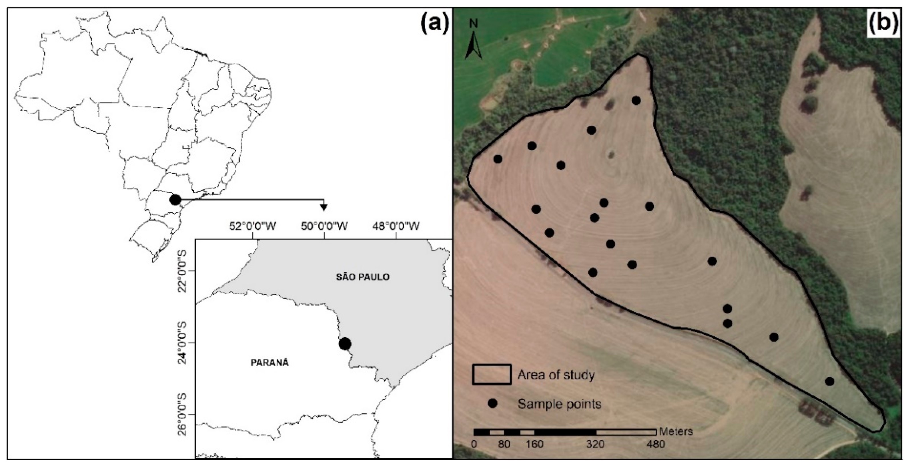
The study was conducted in a 40.1 ha field located in Itararé, São Paulo state, southern Brazil (24°01′36.93″ S–49°25′33.46″ W, 640 m of altitude) (Figure 1). The local climate is defined as a subtropical humid (Cfa) climate according to the Köppen classification [27]. Most rainfall occurs between October and March, with a relatively dry period between April and August. The annual average rainfall is 1532 mm, with mean temperature of 17 °C [28]. The main soil type in the region is a Dystrophic Red-Yellow Oxisol [29], with a sandy clay loam texture. The terrain slope average is 6.28 degrees, which necessitates its cultivation in contours and the use of terraces.
The crop evaluated in the study was maize sown on 18 February 2019 as a second crop with the variety MS30A37PW, with rows spaced in 0.45 m and a final plant population of 63,000 plants ha−1. The area has been under a no-tillage system for more than 30 years and is cultivated under rainfed conditions, with a soybean-maize rotation system during the summer cropping seasons and with wheat (Triticum spp.) or black oat (Avena strigosa Schreb.) during the winter season.
2.2. UAV Thermal Imagery
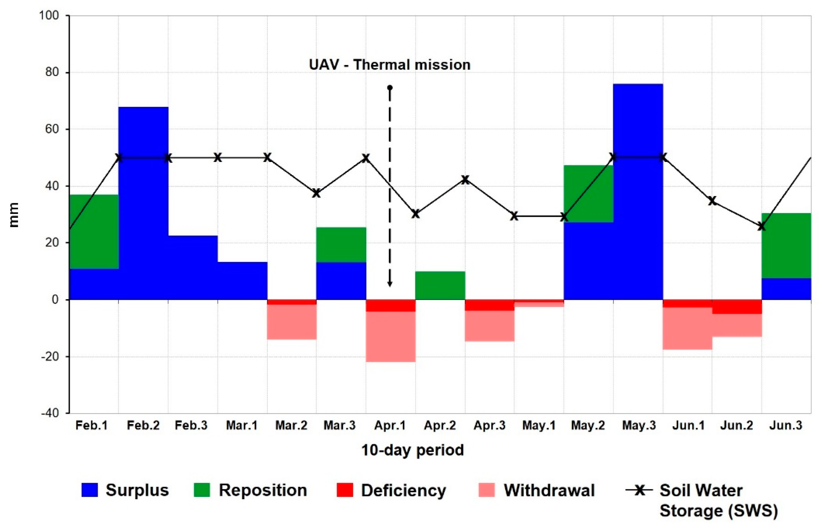
Since the main goal of this study was to assess the ability of thermal imagery in detecting crop water stress, one of the key points was detecting a suitable time during the growing season to collect thermal images. For this reason, we constantly monitored the weather conditions and implemented a soil water balance model to identify periods with water deficiency that would prompt the aerial mission. Other restrictive factors that were imposed were to conduct aerial missions only after canopy closure of the interrow, avoiding soil background effect on thermal infrared (TIR) images, and before senescence, during which time, the water consumption is not significant. Based on these assumptions, the aerial mission was conducted on 2 April 2019, when the maize was at a V12 growth stage and when the canopy was completely closed, and with a soil water deficit of 6.3 mm according to a 10-day serial water balance [30] performed using meteorological data measured by a nearby automated weather station and regional soil parameters (Figure 2).
The flight mission was conducted around two hours past solar noon (between 13:38 and 14:31 local time), which is considered to be the optimal time to evaluate plant water stress [31,32]. There were no clouds during the flight, with a mean air temperature of 30.5 °C, relative humidity of 55%, vapour pressure deficit (VPD) of 1.96 kPa [33], and wind speeds up to 2.5 ms−1.
A low-cost radiometric calibrated FLIR Lepton 3.5 thermal camera (FLIR Systems, Inc., Wilsonville, OR, USA) was used to obtain the aerial images. The camera is composed of an uncooled VOx microbolometer FPA, with a spectral range of 8–14 µm and a resolution of 160 × 120 pixels. Temperature readings are extracted from 14-bit images with a resolution of 0.05 °C and absolute measurement accuracy of ±5 °C or 5% over a range between 10 °C and 140 °C. The camera was attached to a DJI Phantom 4 quadcopter (SZ DJI Technology Co., Shenzhen, China) and was adjusted to collect close to nadir images, being powered up 15 min before flight to ensure proper stabilization time [25] (Kelly et al., 2019). During the flight planning, the parameters were adjusted to deliver images with a forward and side overlap of ≥75% and ≥60%, respectively, at 100 m above ground level, which provided a spatial resolution of 0.63 cm pixel−1.
The image processing necessary to generate the thermal orthomosaic was implemented following the methodology described by Acorsi, Martello, and Gimenez (2020) [34] using the Agisoft Photoscan Professional (v. 1.2.6, Agisoft LLC, St. Petersburg, Russia) to build the orthomosaic. For georeferencing purposes, a total of six ground control points (GCPs) were previously located in the field using distinguishable targets, with their coordinates measured following a post-processing kinematic (PPK) method, using a pair of single-frequency global navigation satellite system (GNSS) receivers (GTR-ABT TechGeo, Brazil).
Once the orthomosaic was finished, it was imported into ArcGIS software (v. 10.2.2, ESRI Ltd., Redlands, CA, USA) along with 18 waypoints corresponding to sampling locations distributed across the field (Figure 1b). The locations were randomly defined within a polygon excluding headland and terrace areas, respecting a minimum and maximum distance between samples of 40 and 200 m, respectively. Circular buffers of a 3 m radius were generated using the sampling location coordinates, which were then used to extract average temperature values from the thermal orthomosaic for each point.
2.3. Field Data
To investigate the relationship between the remotely sensed canopy temperature (CT) and maize water status, we focused on attributes that could explain the water dynamics in the soil. In this sense, we mainly explored the physical attributes from soil that are linked to its capacity to retain water. On the other hand, we also analyzed the plant attributes that are usually affected by long-term drought stress.
2.3.1. Soil Attributes
On the same day that the aerial mission was carried out, soil samples were collected in the layer 0–0.2 m depth at every pre-defined sampling location. The samples were composed of five sub-samples that were distributed within a three-meter radius. The samples were sealed in plastic bags and were taken to a laboratory for further analysis. To determine the gravimetric water content (SGWC), the samples were first weighed and then oven dried at 105 °C for 48 h and were re-weighted to measure the water content that was lost. Moreover, granulometry (Sand; Clay and Silt) and organic matter content were determined according to Teixeira et al. (2017) [35].
After the crop was harvested, undisturbed soil samples were taken at each sampling point from trenches that were 0.12 and 0.35 m in depth with two replications, using metal rings with a dimension of 0.05 × 0.05 m (diameter × height) In the laboratory, the samples were saturated and then weighed. Moreover, the samples were transferred and kept on a tension table with a −6 kPa water potential until mass stabilization, and the samples were then re-weighed. Lastly, the samples were oven dried at 105 °C for 48 h and were then weighed once more. Thus, the macroporosity (MaP) was determined by the mass difference between the saturated samples and samples that were submitted to the −6 kPa water potential, whereas the microporosity (MiP) was obtained from the mass difference between the samples that were obtained at a water potential of at −6 kPa and the oven dried samples [35]. In addition, the bulk density (BD) was also determined, dividing the dry mass of the soil by the volume of the metal ring. The BD information was then used to calculate the soil volumetric water content (SVWC), multiplying the gravimetric water content by BD [36].
Along with the undisturbed soil sampling, soil resistance to penetration (SRP) was also measured in the field within a depth of 0–0.30 m using a handheld digital penetrometer (PLG1020, Falker, Porto Alegre, Brazil). The average SRP values were extracted from 10 sub-samples that had been measured within a three-meter radius of every sampling location and that were positioned between the previous crop rows, with soil moisture content close to field capacity.
Moreover, the soil water holding capacity (SWHC) was calculated according to the model proposed by van Genutchen (1980) [37] using water retention parameters derived from a pedotransfer function (level 3) proposed by Tomasella, Hodnett, and Rossato (2000) [38]. The input variables that were used were the soil texture, organic carbon, and bulk density, with the soil volumetric water content difference between the −10 kPa and −1500 kPa water potentials that were used to represent the SWHC at a 0–0.4 m soil depth.
2.3.2. Plant Attributes
To quantify plant biomass across the field, destructive biomass sampling was carried out at each sampling point right after aerial thermal images were obtained. The process consisted of determining the plant population at each sampling location by counting the number of plants in four 20 m length rows. Among the counted plants, 10 individuals were randomly taken and cut at the soil surface to be immediately weighed using a portable digital balance. The fresh biomass (FBM) was obtained by multiplying the plant average weight measured in the field by the plant population.
When the crop reached physiological maturity (7 July 2019), two rows with a length of 10 m each were manually harvested to measure grain yield at the sampling locations. The ears were threshed, and the grains were oven dried at 65 °C for 48 h to calculate and correct the grain yield (YLD) for a 13% grain moisture.
2.4. Statistical Analysis
Datasets from soil and plant variables including CT were analyzed using the R software (R Development Core Team, 2020), starting with descriptive statistics, calculating the mean, minimum (Min) and maximum (Max) values, standard deviation (SD), coefficient of variation (CV) as well as the skewness and kurtosis values. Furthermore, the normality of the data was checked using the Shapiro–Wilk’s test at 5% significance and when necessary, a Box-Cox transformation was applied to achieve homoscedasticity.
The relationship between the CT and sampled variables was first assessed using a Pearson correlation matrix. Moreover, simple linear regression models were built by relating the CT with the variables that related to the amount of water present in the soil (SVWC). To better understand how CT can contribute to explaining soil water status, other variables that are linked to water dynamics in soil were combined with CT as independent variables in a multiple linear regression at a significance level of 5% (F-test), with predictors being classified according to their importance based on CAR score [39].
3. Results
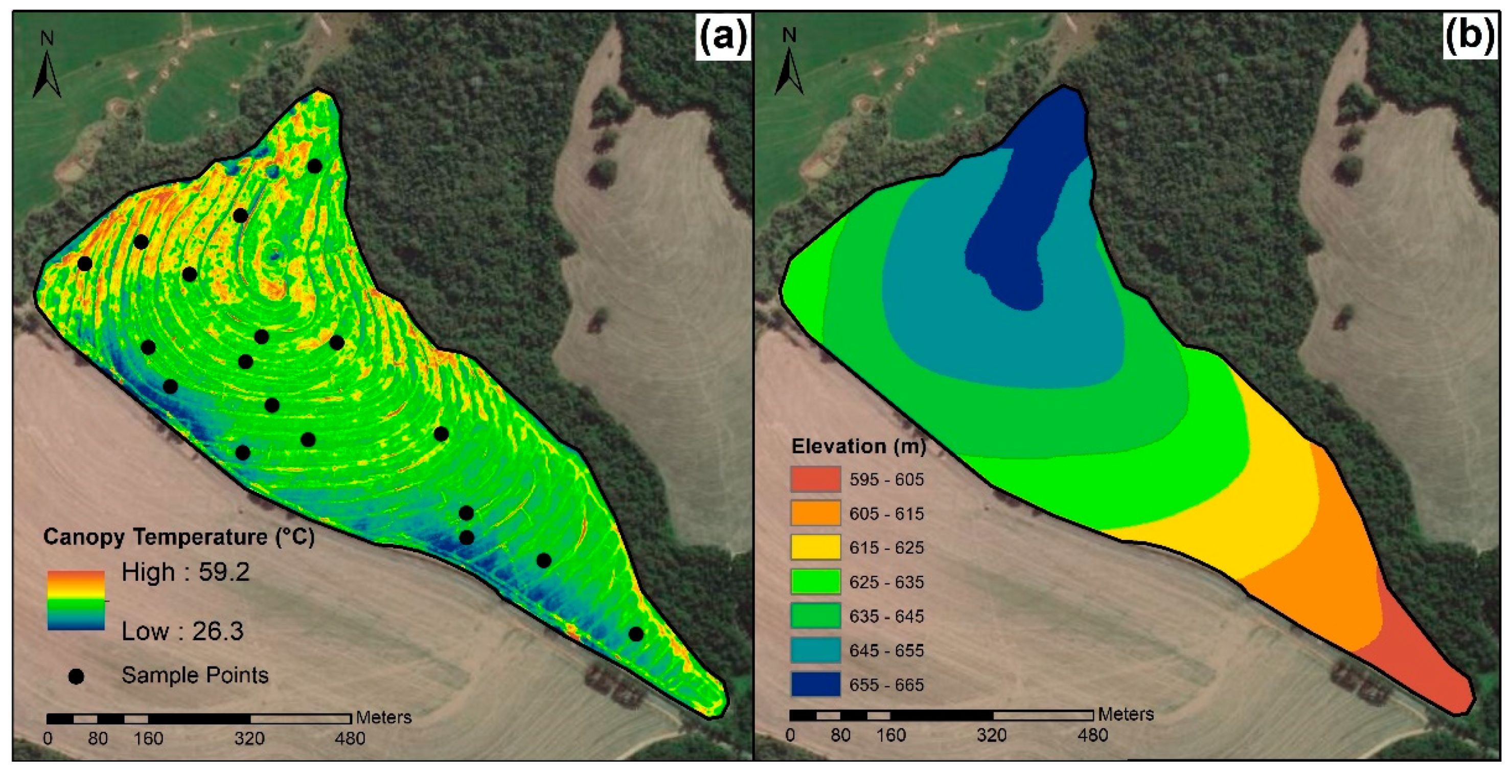
The thermal orthomosaic generated from aerial imagery presented a spatial resolution of 0.63 cm pixel−1, with CT ranging from 23.3 to 59.2 °C across the field (Figure 3). Among the 18 sampling locations, CT varied from 32.8 to 40.6 °C.
Soil and plant attributes sampled in the study generated a total of 15 variables, which are listed in Table 1, including the results of the descriptive statistics. The results showed that silt content, SRP at 0–0.1 m, and macroporosity presented greater variation among soil physical variables, with a CV of 38.1, 28.7, and 23.3%, respectively. This variability reflects on SWHC, which ranged from 41.1 to 72.4 mm and on SVWC measurements, indicating that soil moisture content varied between 0.15 and 0.22 m3 m−3 during the flight campaign.
The Pearson’s correlations among the studied variables are listed in Table 2. As expected, CT was negatively correlated with most variables (Sand, Clay, OM, MaP, SVWC, SWHC, FBM, and YLD), indicating that higher temperature readings can be linked to lower values on these attributes. Significant correlation values (p-value ≤ 0.05) were obtained when relating CT with SVWC, SRP at 0–0.1 m, and FBM, with Pearson correlation values of −0.65, 0.58, and −0.56, respectively.
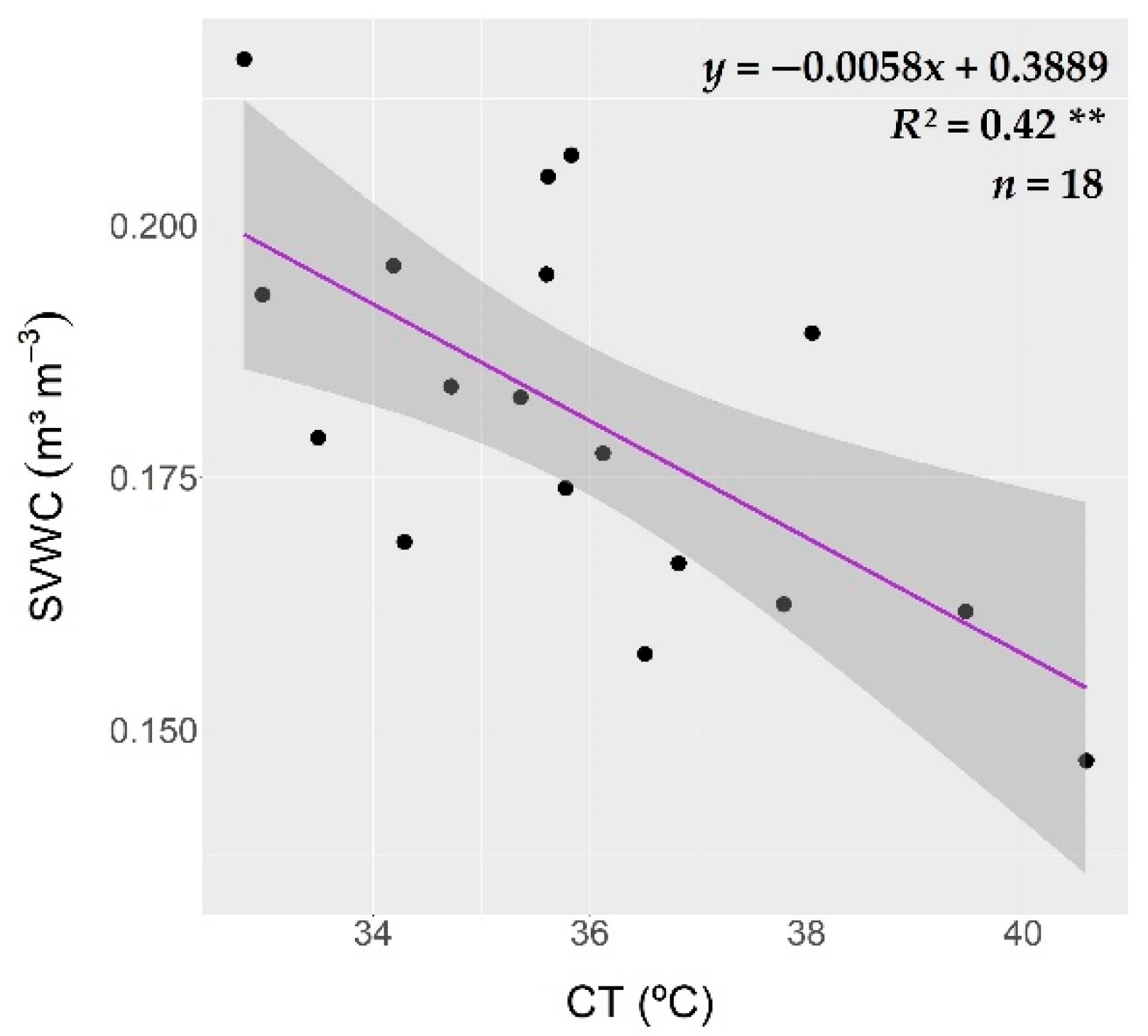
In order to test the feasibility of predicting the soil water content using CT information, we first implemented simple linear regression with SVWC as an independent variable (Figure 4). The results showed that the linear regression model was statistically significant, with a p-value lower than 0.01 and an R2 of 0.42.
Moreover, a multiple linear regression was performed by combining CT and all of the soil physical parameters sampled as independent variables with SVWC as the dependent variable. The regression results are shown in Table 3, demonstrating that by adding soil physical variables, the multiple linear regression model achieved an R2 of 0.88 (p-value ≤ 0.05). The importance of each predictor in the multiple regression model was determined based on a CAR score [39] in which the clay content, CT, and SRP at 0.2–0.3 m were the most important variables for the prediction SVWC, with CAR values of 0.289, 0.286, and 0.240, respectively.
4. Discussion
Since the main goal of the study was to assess the suitability of remotely sensed CT on predicting maize water status, the data acquisition and image processing that were employed focused on delivering precise and accurate temperature measurements. According to Mesas-Carrascosa et al. (2018) [40], accuracies around 1 °C are ideal when analyzing crop water status with thermal cameras, which is similar to reported values obtained with the same instrument and methodology employed in our study, where an accuracy of 1.32 °C (RMSE) and R2 of 0.99 were observed under equivalent conditions [34].
Another important aspect regarding plant water status assessment using CT is the timing for data acquisition. In general, CT is a function of the evapotranspiration rate, which depends on the atmospheric evaporative demand and soil water storage [41]. Considering the VPD of 1.96 kPa measured during image acquisition, the meteorological condition was not restricting the evapotranspiration rate of the plants [42,43,44], and therefore, CT would be mainly influenced by the soil water status. Results from the 10-day soil water balance calculated with SWHC adjusted for each sampling location revealed a water deficiency between 3.0 and 5.8 mm during this period, which was confirmed by the soil sampling that was carried out while aerial images were taken. The SVWC results varied from 0.15 to 0.22 m3 m−3 and compared well with the SVWC values at the permanent wilting point (1500 kPa), which, according to the pedotransfer function employed to estimate SWHC, varies between 0.13 and 0.20 m3 m−3 among the sampling locations.
In addition to soil water deficit and VPD condition, the timing for thermal image acquisition tends to be key when assessing crop water stress. For this reason, the aerial imagery was carried out close to noontime, which is the time of the day when the leaf water potential and stomatal conductance tend to be the lowest, resulting in maximum expression of stress [20,31], which is also when the CT readings between 32.81 and 40.58 °C were measured. Similar values were observed by DeJonge et al. (2015) [45] when assessing maize water stress using CT in northern Colorado, USA, where the treatments with higher induced water stress presented an average temperature of 31 °C, ranging up to 39 °C during the vegetative stage. Moreover, Zhang et al. (2019) [15] also obtained corresponding results while assessing different levels of irrigation in maize during the late vegetative stage in China, with CT readings varying from 33.2 to 40.1 °C on treatments where irrigation restriction was applied.
In comparison to temperature readings from sampling locations, the field-scale CT presented a wider range of values, varying from 26.3 to 59.2 °C. Zhang et al. (2019) [15] reported similar results from a maize field thermal orthomosaic, with CT values starting around 20 °C ranging up to 60 °C. According to the authors, portions of the field with higher CT values occurred due to severe water stress, in which plants with curled leaves were more frequent. When the leaves are curled, the leaf area index is reduced, and that might increase the proportion of soil pixels that are able to be detected by the sensor, resulting in higher temperature values being extracted from the thermal images. The presence of terraces was found to be the main cause of the higher temperature values observed across the field, in which the accumulation of water from rainfall that occurred during early growth stages reduced the plant population dramatically on the upper portion of some terraces, with temperature readings mainly being influenced the by soil. On the other hand, lower CT readings were more prominent on flatter portions of the field and lower altitudes, where the water accumulation tends to be higher.
The Pearson’s correlation analysis relating CT with plant variables was based on fresh biomass (FBM) and grain yield (YLD). Negative correlation values were obtained for both variables, with −0.56 for FBM and −0.45 for YLD. Similar values were reported by Bhandari (2016) [46] in a study assessing different maize hybrids under dryland conditions in north Texas, USA, with Person’s correlation values between −0.32 and −0.64 when comparing CT and FBM. Moreover, comparable results regarding the relationship between CT and YLD were observed by Zia et al. (2013) [47] during experiments with different maize genotypes in Mexico, achieving a correlation value of −0.55.
Among the physical attributes of the soil, the clay content (r = −0.44), macroporosity (r = −0.45), and SRP (r = 0.21 to 0.58) yielded the highest correlation values. These variables were well correlated with SVWC, presenting Pearson’s correlation values of 0.61, 0.37, and −0.40, respectively. The results corroborate the simple linear regression model obtained by plotting CT against SVWC, where the linear relationship was statistically significant with an R2 of 0.42, demonstrating that CT tends to increase when the soil water content is reduced. The correlation was somewhat weaker in comparison to the values that were reported by Zhang et al. (2019) [15], in which the linear regression models between SVWC at 0–0.2 m soil depth and CT yielded R2 values between 0.40 and 0.53. The higher R2 values can be explained by the treatments that were tested in their study, where five levels of irrigation were applied, ranging from fully irrigated to severe deficit irrigation, resulting in a wider range of soil water contents during the assessment, which contributed to obtaining regression models with well-distributed points favoring higher correlation values. Even though the correlation value obtained with SVWC indicates that predicting soil water content using CT may lead to substantial errors, thermal orthomosaics can be used to understand the spatial variability of soil water content, helping to identify regions within the field with lower and higher SVWC.
When the CT was associated with soil physical attributes in a multiple linear regression model with SVWC set as the dependent variable, the prediction performance increased significantly, achieving an R2 value of 0.88. According to the CAR score [39], which classifies the importance of independent variables in multiple regressions, CT was the second most important variable (CAR = 0.286) among the 11 attributes that were included in the model, along with clay content (CAR = 0.289) and SRP at the 0.2–0.3 m soil depth (CAR = 0.240). This result indicates the benefit of including CT on crop water status assessments, even when the soil physical attributes that are directly related to soil water dynamics are available. While the physical attributes of soil tend to be more stable over time, CT presents high temporal variability, matching the needs of in-season analysis.
5. Conclusions
From UAV-based thermal imagery, we were able to generate a thermal orthomosaic representing the spatial variability of a rainfed maize canopy temperature along a field of 40.1 ha. Among the sampling locations, temperature readings varied from 32.81 to 40.58 °C, indicating different levels of plant drought stress across the field.
Exploring the hypothesis that canopy temperature is primarily a function of soil water storage, soil sampling was carried out to determine the soil water content and other key variables that could be directly related to soil water content. The results indicated that canopy temperature alone is not sufficient to predict soil water status (R2 = 0.42). Alternatively, the performance of soil water status prediction was substantially increased when the thermal data were associated with soil physical attributes (R2 = 0.88), demonstrating a combination that can be used as an in-season tool for onset drought stress assessments.
Author Contributions
M.G.A. and L.M.G. conceived the idea; M.G.A. and L.M.G. designed and performed the experiments; M.G.A. analyzed the data. Both authors contributed to the writing and the editing of the manuscript. All authors have read and agreed to the published version of the manuscript.
Funding
We thank the Coordination for the Improvement of Higher Education Personnel (CAPES) for providing the scholarship to M.G.A. (grant: 8882.378424/2019-01).
Acknowledgments
The authors would like to thank Gilmar Martinelli Junior, Matheus Fontana Westphalen e Marcio Melquiades Silva dos Anjos for assisting throughout all the data collection; the Abc Foundation for sharing the historic data from the field studied; Fabio Cunha for granting free access to the field where this study was developed; Peterson Ricardo Fiorio, for lending us his own UAV platform multiple times; Rodrigo Gonçalves Trevisan, Mauricio Martello, and Tarik Marques Tanure for supporting the Lepton camera construction; Áureo Santana de Oliveira and Juarez Renó do Amaral for all of the technical assistance with the electronic instrumentation; and the SmartAgri company for access to a 3D printer used for camera construction.
Conflicts of Interest
The authors declare no conflict of interest.
References
- Lambers, H.; Chapin, F.S.; Pons, T.L. Plant Physiological Ecology; Springer: New York, NY, USA, 2008; ISBN 978-0-387-78340-6. [Google Scholar]
- Gautam, D.; Pagay, V. A Review of Current and Potential Applications of Remote Sensing to Study the Water Status of Horticultural Crops. Agronomy 2020, 10, 140. [Google Scholar] [CrossRef] [Green Version]
- Fedoroff, N.V.; Battisti, D.S.; Beachy, R.N.; Cooper, P.J.; Fischhoff, D.A.; Hodges, C.N.; Knauf, V.C.; Lobell, D.; Mazur, B.J.; Molden, D.; et al. Radically rethinking agriculture for the 21st century. Science 2010, 327, 833–834. [Google Scholar] [CrossRef] [Green Version]
- Gebbers, R.; Adamchuk, V.I. Precision agriculture and food security. Science 2010, 327, 828–831. [Google Scholar] [CrossRef] [PubMed]
- Mulla, D.J. Twenty five years of remote sensing in precision agriculture: Key advances and remaining knowledge gaps. Biosyst. Eng. 2013, 114, 358–371. [Google Scholar] [CrossRef]
- Maes, W.H.; Steppe, K. Perspectives for remote sensing with unmanned aerial vehicles in precision agriculture. Trends Plant Sci. 2019, 24, 152–164. [Google Scholar] [CrossRef]
- Mulla, D.J.; McBratney, A.B. Soil spatial variability. In Handbook of Soil Science; Sumner, M.E., Ed.; CRS Press: Boca Raton, FL, USA, 2000; pp. 321–352. [Google Scholar]
- Heiskanen, J.; Mäkitalo, K. Soil water-retention characteristics of Scots pine and Norway spruce forest sites in Finnish Lapland. For. Ecol. Manag. 2002, 162, 137–152. [Google Scholar] [CrossRef]
- Sobieraj, J.A.; Elsenbeer, H.; Cameron, G. Scale dependency in spatial patterns of saturated hydraulic conductivity. Catena 2004, 55, 49–77. [Google Scholar] [CrossRef]
- Iqbal, J.; Thomasson, J.A.; Jenkins, J.N.; Owens, P.R.; Whisler, F.D. Spatial variability analysis of soil physical properties of alluvial soils. Soil Sci. Soc. Am. J. 2005, 69, 1338. [Google Scholar] [CrossRef]
- Idso, S.B.; Jackson, R.D.; Pinter, P.J., Jr.; Reginato, R.J.; Hatfield, J.L. Normalizing the stress-degree-day parameter for environmental variability. Agric. Meteorol. 1981, 24, 45–55. [Google Scholar] [CrossRef]
- Jones, H.G. Irrigation scheduling: Advantages and pitfalls of plant-based methods. J. Exp. Bot. 2004, 55, 2427–2436. [Google Scholar] [CrossRef] [PubMed] [Green Version]
- Gago, J.; Douthe, C.; Coopman, R.; Gallego, P.; Ribas-Carbo, M.; Flexas, J.; Escalona, J.; Medrano, H. UAVs challenge to assess water stress for sustainable agriculture. Agric. Water Manag. 2015, 153, 9–19. [Google Scholar] [CrossRef]
- Jackson, R.D.; Idso, S.B.; Reginato, R.J.; Pinter, P.J., Jr. Canopy temperature as a crop water stress indicator. Water Resour. Res. 1981, 17, 1133–1138. [Google Scholar] [CrossRef]
- Zhang, L.; Niu, Y.; Zhang, H.; Han, W.; Li, G.; Tang, J.; Peng, X. Maize canopy temperature extracted from UAV thermal and RGB imagery and its application in water stress monitoring. Front. Plant Sci. 2019, 10, 1270. [Google Scholar] [CrossRef] [PubMed]
- Crusiol, L.G.T.; Nanni, M.R.; Furlanetto, R.H.; Sibaldelli, R.N.R.; Cezar, E.; Mertz-Henning, L.M.; Nepomuceno, A.L.; Neumaier, N.; Farias, J.R.B. UAV-based thermal imaging in the assessment of water status of soybean plants. Int. J. Remote Sens. 2020, 41, 3243–3265. [Google Scholar] [CrossRef]
- Bian, J.; Zhang, Z.; Chen, J.; Chen, H.; Cui, C.; Li, X.; Chen, S.; Fu, Q. Simplified Evaluation of Cotton Water Stress Using High Resolution Unmanned Aerial Vehicle Thermal Imagery. Remote Sens. 2019, 11, 267. [Google Scholar] [CrossRef] [Green Version]
- Zhou, J.; Khot, L.R.; Boydston, R.A.; Miklas, P.N.; Porter, L. Low altitude remote sensing technologies for crop stress monitoring: A case study on spatial and temporal monitoring of irrigated pinto bean. Precis. Agric. 2018, 19, 555–569. [Google Scholar] [CrossRef]
- Zarco-Tejada, P.J.; González-Dugo, V.; Berni, J.A.J. Fluorescence, temperature and narrow-band indices acquired from a UAV platform for water stress detection using a micro-hyperspectral imager and a thermal camera. Remote Sens. Environ. 2012, 117, 322–337. [Google Scholar] [CrossRef]
- Bellvert, J.; Zarco-Tejada, P.J.; Girona, J.; Fereres, E. Mapping crop water stress index in a ‘Pinot-noir’ vineyard: Comparing ground measurements with thermal remote sensing imagery from an unmanned aerial vehicle. Precis. Agric. 2014, 15, 361–376. [Google Scholar] [CrossRef]
- Matese, A.; Baraldi, R.; Berton, A.; Cesaraccio, C.; Di Gennaro, S.F.; Duce, P.; Facini, O.; Mameli, M.G.; Piga, A.; Zaldei, A. Estimation of Water Stress in Grapevines Using Proximal and Remote Sensing Methods. Remote Sens. 2018, 10, 114. [Google Scholar] [CrossRef] [Green Version]
- Berni, J.; Zarco-Tejada, P.; Suarez, L.; Fereres, E. Thermal and narrowband multispectral remote sensing for vegetation monitoring from an unmanned aerial vehicle. IEEE Trans. Geosci. Remote Sens. 2009, 47, 722–738. [Google Scholar] [CrossRef] [Green Version]
- Klemas, V.V. Coastal and Environmental Remote Sensing from Unmanned Aerial Vehicles: An Overview. J. Coast. Res. 2015, 31, 1260–1267. [Google Scholar] [CrossRef] [Green Version]
- Aubrecht, D.M.; Helliker, B.R.; Goulden, M.L.; Roberts, D.A.; Still, C.J.; Richardson, A.D. Continuous, long-term, high-frequency thermal imaging of vegetation: Uncertainties and recommended best practices. Agric. For. Meteorol. 2016, 228, 315–326. [Google Scholar] [CrossRef] [Green Version]
- Kelly, J.; Kljun, N.; Olsson, P.-O.; Mihai, L.; Liljeblad, B.; Weslien, P.; Klemedtsson, L.; Eklundh, L. Challenges and Best Practices for Deriving Temperature Data from an Uncalibrated UAV Thermal Infrared Camera. Remote Sens. 2019, 11, 567. [Google Scholar] [CrossRef] [Green Version]
- Radoglou-Grammatikis, P.; Sarigiannidis, P.; Lagkas, T.; Moscholios, I. A compilation of UAV applications for precision agriculture. Comput. Netw. 2020, 172, 107148. [Google Scholar] [CrossRef]
- Alvares, C.A.; Stape, J.L.; Sentelhas, P.C.; de Moraes Gonçalves, J.L.; Sparovek, G. Köppen’s climate classification map for Brazil. Meteorol. Z. 2013, 22, 711–728. [Google Scholar] [CrossRef]
- Tremocoldi, W.A.; Brunini, O. Caracterização agroclimática das unidades da Secretaria de Agricultura e Abastecimento do Estado de São Paulo: Capão Bonito e região. Bol. Téc. Inst. Agron. Camp. 2008, 205, 30. [Google Scholar]
- Rossi, M. Mapa Pedológico do Estado de São Paulo: Revisado e Ampliado; Instituto Florestal (Florestal Institute): São Paulo, Brazil, 2017; Volume 1, ISBN 3239660180. [Google Scholar]
- Thornthwaite, C.W.; Mather, J.R. The Water Balance; Laboratory in Climatology, Johns Hopkins University: Baltimore, MD, USA, 1955; Volume 8, pp. 1–104. [Google Scholar]
- Alchanatis, V.; Cohen, Y.; Cohen, S.; Moller, M.; Sprinstin, M.; Meron, M.; Tspiris, J.; Saranga, Y.; Sela, E. Evaluation of different approaches for estimating and mapping crop water status in cotton with thermal imaging. Precis. Agric. 2010, 11, 27–41. [Google Scholar] [CrossRef]
- Lu, Z.; Percy, R.G.; Qualset, C.O.; Zeiger, E. Stomatal conductance predicts yields in irrigated Pima cotton and bread wheat grown at high temperatures. J. Exp. Bot. 1998, 49, 453–460. [Google Scholar] [CrossRef] [Green Version]
- Anderson, D.B. Relative humidity or vapor pressure deficit. Ecology 1936, 17, 277–282. [Google Scholar] [CrossRef]
- Acorsi, M.G.; Gimenez, L.M.; Martello, M. Assessing the Performance of a Low-Cost Thermal Camera in Proximal and Aerial Conditions. Remote Sens. 2020, 12, 3591. [Google Scholar] [CrossRef]
- Teixeira, P.C.; Donagemma, G.K.; Fontana, A.; Teixeira, W.G. Manual de Métodos de Análise de Solos, 3rd ed.; Revisada e Ampliada; Embrapa: Brasília, Brazil, 2017; ISBN 978-85-7035-771-7. [Google Scholar]
- Dirksen, C. Soil Physics Measurements; Catena: Reiskirchen, Germany, 1999; ISBN 3923381433. [Google Scholar]
- Van Genuchten, M.T. A closed-form equation for predicting the hydraulic conductivity of unsaturated soils. Soil. Sci. Soc. Am. J. 1980, 44, 892–898. [Google Scholar] [CrossRef] [Green Version]
- Tomasella, J.; Hodnett, M.G.; Rossato, L. Pedotransfer Functions for the Estimation of Soil Water Retention in Brazilian Soils. Soil Sci. Soc. Am. J. 2000, 64, 327–338. [Google Scholar] [CrossRef]
- Zuber, V.; Strimmer, K. High-dimensional regression and variable selection by using CAR scores. Stat. Appl. Genet. Mol. Biol. 2011, 10, 1. [Google Scholar] [CrossRef] [Green Version]
- Mesas-Carrascosa, F.J.; Pérez-Porras, F.; de Larriva, J.E.M.; Frau, C.M.; Agüera-Vega, F.; Carvajal-Ramírez, F.; Martínez-Carricondo, P.; García-Ferrer, A. Drift correction of lightweight microbolometer thermal sensors on-board unmanned aerial vehicles. Remote Sens. 2018, 10, 615. [Google Scholar] [CrossRef] [Green Version]
- Khanal, S.; Fulton, J.; Shearer, S. An overview of current and potential applications of thermal remote sensing in precision agriculture. Comput. Electron. Agric. 2017, 139, 22–32. [Google Scholar] [CrossRef]
- O’Toole, J.C.; Real, J.G. Estimation of aerodynamic and crop resistances from canopy temperature. Agron. J. 1986, 78, 305–310. [Google Scholar] [CrossRef]
- Gholipoor, M.; Choudhary, S.; Sinclair, T.R.; Messina, C.D.; Cooper, M. Transpiration response of maize hybrids to atmospheric vapor pressure deficit. J. Agron. Crop Sci. 2013, 199, 155–160. [Google Scholar] [CrossRef]
- Yang, Z.; Sinclair, T.R.; Zhu, M.; Messina, C.D.; Cooper, M.; Hammer, G.L. Temperature effect on transpiration response of maize plants to vapour pressure deficit. Environ. Exp. Bot. 2012, 78, 157–162. [Google Scholar] [CrossRef]
- DeJonge, K.C.; Taghvaeian, S.; Trout, T.J.; Comas, L.H. Comparison of canopy temperature-based water stress indices for maize. Agric. Water Manag. 2015, 156, 51–62. [Google Scholar] [CrossRef]
- Bhandari, M. Use of Infrared Thermal Imaging for Estimating Canopy Temperature in Wheat and Maize. Master’s Thesis, West Texas A&M University, Canyon, TX, USA, 13 September 2016. Available online: https://wtamu-ir.tdl.org/handle/11310/133 (accessed on 5 October 2021).
- Zia, S.; Romano, G.; Spreer, W.; Sanchez, C.; Cairns, J.; Araus, J.; Müller, J. Infrared thermal imaging as a rapid tool for identifying water-stress tolerant maize genotypes of different phenology. J. Agron. Crop Sci. 2013, 199, 75–84. [Google Scholar] [CrossRef]
Figure 1.
Study field location (a) with soil and plant sampling points (b).

Figure 2.
Climatological water balance [30] calculated in a ten-day time step and considering 50 mm of soil water holding capacity. The dashed line indicates the UAV mission conducted on 2 April 2019.
Figure 2.
Climatological water balance [30] calculated in a ten-day time step and considering 50 mm of soil water holding capacity. The dashed line indicates the UAV mission conducted on 2 April 2019.

Figure 3.
Canopy temperature orthomosaic obtained with aerial thermal imaging (a) and hypsometric map of the experimental field (b).
Figure 3.
Canopy temperature orthomosaic obtained with aerial thermal imaging (a) and hypsometric map of the experimental field (b).

Figure 4.
Linear regression model between canopy temperature (CT) and soil volumetric water content (SVWC). R2 = coefficient of determination; n = number of samples; correlation was significant at 0.01 probability level (**).
Figure 4.
Linear regression model between canopy temperature (CT) and soil volumetric water content (SVWC). R2 = coefficient of determination; n = number of samples; correlation was significant at 0.01 probability level (**).


Table 1.
Descriptive statistics of the soil and plant attributes extracted from the sampling locations.
Table 1.
Descriptive statistics of the soil and plant attributes extracted from the sampling locations.
| Variables | Abbrev | Unit | n | Mean | Min | Max | SD | CV (%) | Skew | Kurt |
|---|---|---|---|---|---|---|---|---|---|---|
| Sand | - | % | 18 | 54.34 | 45.10 | 59.70 | 4.48 | 8.05 | −1.10 | 0.17 |
| Clay | - | % | 18 | 29.42 | 22.30 | 37.30 | 4.46 | 15.04 | 0.55 | −0.37 |
| Silt | - | % | 18 | 16.24 | 7.80 | 29.60 | 5.87 | 38.10 | 0.58 | 0.09 |
| Organic Matter | OM | % | 18 | 2.72 | 1.90 | 4.20 | 0.49 | 18.29 | 1.47 | 4.23 |
| Microporosity | MiP | m3 m−3 | 18 | 0.32 | 0.28 | 0.35 | 0.02 | 6.79 | 0.22 | −0.63 |
| Macroporosity | MaP | m3 m−3 | 18 | 0.06 | 0.04 | 0.08 | 0.01 | 23.25 | 0.18 | −0.62 |
| Bulk Density | BD | Mg m−3 | 18 | 1.44 | 1.26 | 1.59 | 0.08 | 5.50 | −0.38 | 0.79 |
| Soil Resistance to Penetration (0–0.1 m) | SRP0–0.1m | KPa | 18 | 1000.98 | 572.25 | 1698.45 | 289.96 | 28.70 | 0.57 | 0.39 |
| Soil Resistance to Penetration (0.1–0.2 m) | SRP0.1–0.2m | KPa | 18 | 2167.81 | 1681.40 | 2602.90 | 258.08 | 12.17 | 0.01 | −0.97 |
| Soil Resistance to Penetration (0.2–0.3 m) | SRP0.2–0.3m | KPa | 18 | 1928.53 | 1583.15 | 2449.40 | 229.27 | 12.29 | 0.60 | −0.12 |
| Soil Volumetric Water Content | SVWC | m3 m−3 | 18 | 0.18 | 0.15 | 0.22 | 0.02 | 10.39 | 0.08 | −0.63 |
| Soil Water Holding Capacity | SWHC | mm | 18 | 51.61 | 41.10 | 72.41 | 7.92 | 15.96 | 1.13 | 1.39 |
| Fresh Biomass | FBM | Mg ha−1 | 18 | 30.43 | 17.80 | 36.54 | 5.41 | 17.60 | −1.27 | 1.41 |
| Grain Yield | YLD | Mg ha−1 | 18 | 9.14 | 6.98 | 11.45 | 1.26 | 13.70 | −0.18 | −0.69 |
| Canopy Temperature | CT | °C | 18 | 35.89 | 32.81 | 40.58 | 2.11 | 5.90 | 0.63 | 0.21 |
Abbrev = abbreviation; n = number of samples; Min = minimum value observed; Max = maximum value observed; SD = standard deviation; CV = coefficient of variation; Skew = skewness; Kurt = kurtosis.
Table 2.
Pearson’s correlation matrix between soil and plant attributes extracted from the sampling locations.
Table 2.
Pearson’s correlation matrix between soil and plant attributes extracted from the sampling locations.
| Sand | Clay | Silt | OM | MiP | MaP | BD | SRP0–0.1m | SRP0.1–0.2m | SRP0.2–0.3m | SVWC | SWHC | FBM | YLD | CT | |
|---|---|---|---|---|---|---|---|---|---|---|---|---|---|---|---|
| Sand | 1 | −0.14 | −0.65 ** | 0.31 | −0.75 *** | 0.40 | 0.11 | −0.13 | 0.04 | −0.29 | −0.01 | −0.16 | 0.28 | 0.18 | −0.05 |
| Clay | 1 | −0.65 ** | 0.09 | 0.51 * | 0.55 * | −0.79 *** | −0.29 | −0.28 | −0.50 * | 0.61 ** | 0.86 *** | 0.13 | −0.32 | −0.44 | |
| Silt | 1 | −0.31 | 0.19 | −0.72 *** | 0.52 * | 0.32 | 0.18 | 0.60 ** | −0.46 | −0.53 * | −0.31 | 0.11 | 0.37 | ||
| OM | 1 | −0.29 | 0.37 | −0.13 | −0.37 | −0.09 | −0.16 | 0.13 | 0.17 | 0.36 | 0.03 | −0.13 | |||
| MiP | 1 | −0.09 | −0.48 * | 0.34 | 0.17 | 0.00 | 0.10 | 0.54 * | −0.41 | −0.45 | 0.05 | ||||
| MaP | 1 | −0.79 *** | −0.31 | −0.31 | −0.68 ** | 0.37 | 0.63 ** | 0.22 | 0.06 | −0.45 | |||||
| BD | 1 | 0.15 | 0.28 | 0.60 ** | −0.34 | −0.88 *** | 0.01 | 0.24 | 0.34 | ||||||
| SRP0–0.1m | 1 | 0.83 *** | 0.22 | −0.40 | −0.26 | −0.47 * | −0.15 | 0.58 * | |||||||
| SRP0.1–0.2m | 1 | 0.30 | −0.27 | −0.31 | −0.20 | 0.09 | 0.47 | ||||||||
| SRP0.2–0.3m | 1 | −0.55 * | −0.50 * | −0.25 | 0.30 | 0.21 | |||||||||
| SVWC | 1 | 0.42 | 0.64 ** | 0.15 | −0.65 ** | ||||||||||
| SWHC | 1 | 0.10 | −0.31 | −0.45 | |||||||||||
| FBM | 1 | 0.51 * | −0.56 * | ||||||||||||
| YLD | 1 | −0.45 | |||||||||||||
| CT | 1 | ||||||||||||||
Correlation was significant at 0.001 (***); 0.01 (**); and 0.05 (*) probability levels.
Table 3.
Multiple linear regression model obtained to estimate soil volumetric water content (SVWC) using soil physical parameters and canopy temperature (CT).
Table 3.
Multiple linear regression model obtained to estimate soil volumetric water content (SVWC) using soil physical parameters and canopy temperature (CT).
| Estimate | Std. Error | t Value | Pr(>|t|) | CAR | |
|---|---|---|---|---|---|
| (Intercept) | −14.2500 | 10.8539 | −1.313 | 0.237 | - |
| Sand | 0.0145 | 0.0110 | 1.319 | 0.235 | 0.003 |
| Clay | 0.0154 | 0.0113 | 1.361 | 0.222 | 0.289 |
| Silt | 0.0148 | 0.0111 | 1.336 | 0.230 | 0.008 |
| OM | 6.3 × 10⁻⁴ | 7.79 × 10⁻⁴ | 0.814 | 0.447 | 0.004 |
| MiP | −0.9592 | 0.7168 | −1.338 | 0.229 | 0.000 |
| MaP | −0.2889 | 0.8593 | −0.336 | 0.748 | 0.004 |
| BD | 0.1102 | 0.1569 | 0.703 | 0.509 | 0.008 |
| SRP0–0.1m | 3.77 × 10⁻⁵ | 3.79 × 10⁻⁵ | 0.994 | 0.359 | 0.037 |
| SRP0.1–0.2m | 1.29 × 10⁻⁶ | 2.75 × 10⁻⁵ | 0.047 | 0.964 | 0.000 |
| SRP0.2–0.3m | −5.82 × 10⁻⁵ | 1.76 × 10⁻⁵ | −3.316 | 0.016 | 0.240 |
| CT | −0.0039 | 0.0021 | −1.899 | 0.106 | 0.286 |
| R2 multiple | 0.88 | ||||
| F test (p-value) | 0.05 | ||||
| Shapiro–Wilk (p-value) | 0.77 | ||||
Publisher’s Note: MDPI stays neutral with regard to jurisdictional claims in published maps and institutional affiliations. |
© 2021 by the authors. Licensee MDPI, Basel, Switzerland. This article is an open access article distributed under the terms and conditions of the Creative Commons Attribution (CC BY) license (https://creativecommons.org/licenses/by/4.0/).
Share and Cite
MDPI and ACS Style
Acorsi, M.G.; Gimenez, L.M. Predicting Soil Water Content on Rainfed Maize through Aerial Thermal Imaging. AgriEngineering 2021, 3, 942-953. https://0-doi-org.brum.beds.ac.uk/10.3390/agriengineering3040059
AMA Style
Acorsi MG, Gimenez LM. Predicting Soil Water Content on Rainfed Maize through Aerial Thermal Imaging. AgriEngineering. 2021; 3(4):942-953. https://0-doi-org.brum.beds.ac.uk/10.3390/agriengineering3040059
Chicago/Turabian StyleAcorsi, Matheus Gabriel, and Leandro Maria Gimenez. 2021. "Predicting Soil Water Content on Rainfed Maize through Aerial Thermal Imaging" AgriEngineering 3, no. 4: 942-953. https://0-doi-org.brum.beds.ac.uk/10.3390/agriengineering3040059