Article

Prospective Fault Displacement Hazard Assessment for Leech River Valley Fault Using Stochastic Source Modeling and Okada Fault Displacement Equations

by
Katsuichiro Goda
1,2,* and
Parva Shoaeifar
1
1
Department of Earth Sciences, Western University, London, ON N6A 3K7, Canada
2
Department of Statistical & Actuarial Sciences, Western University, London, ON N6A 3K7, Canada
*
Author to whom correspondence should be addressed.
Submission received: 18 March 2022 / Revised: 19 May 2022 / Accepted: 20 May 2022 / Published: 21 May 2022

Abstract

:
In this study, an alternative method for conducting probabilistic fault displacement hazard analysis is developed based on stochastic source modeling and analytical formulae for evaluating the elastic dislocation due to an earthquake rupture. It characterizes the uncertainty of fault-rupture occurrence in terms of its position, geometry, and slip distribution and adopts so-called Okada equations for the calculation of fault displacement on the ground surface. The method is compatible with fault-source-based probabilistic seismic hazard analysis and can be implemented via Monte Carlo simulations. The new method is useful for evaluating the differential displacements caused by the fault rupture at multiple locations simultaneously. The proposed method is applied to the Leech River Valley Fault located in the vicinity of Victoria, British Columbia, Canada. Site-specific fault displacement and differential fault displacement hazard curves are assessed for multiple sites within the fault-rupture zone. The hazard results indicate that relatively large displacements (∼0.5 m vertical uplift) can be expected at low probability levels of 10−4. For critical infrastructures, such as bridges and pipelines, quantifying the uncertainty of fault displacement hazard is essential to manage potential damage and loss effectively.

1. Introduction

Surface fault rupture can cause catastrophic damage to engineering structures and lifeline systems built across or near an active fault [1]. Ground surface deformation is critical in designing nuclear power plants and the installation procedure of nuclear facilities [2,3]. Surface displacement hazards due to earthquakes can have a major influence in assessing financial risk related to the closure of business facilities and utility service interruptions. Moreover, the consequences of these failures are not only life-threatening but also have adverse impacts on the environment, such as air/water contamination [4,5]. Various methodologies for characterizing the fault displacement hazard have been developed to quantify the impacts of major ground deformation events.
A general methodology of probabilistic fault displacement hazard analysis (PFDHA) was proposed by [6] for normal faulting earthquakes and was applied to the Wasatch Fault in central Utah and the Yucca Mountain nuclear waste repository in Nevada [7]. The fault displacement hazard is quantified with the earthquake-based and displacement-based approaches. The former utilizes a conventional probabilistic seismic hazard analysis (PSHA) framework [8,9], substituting ground motion prediction equations with displacement prediction equations for on-fault and off-fault surface ruptures. The latter defines the rate of exceeding a given displacement by combining the frequency of rupture occurrence and the fault displacement distribution, directly from seismological and geological information at the site of interest. The earthquake approach was also extended for reverse and strike-slip faults in Japan [10].
Empirical predictive relationships are the key component of conventional PFDHA methodologies describing the geometry and slip distribution of earthquake ruptures (e.g., along-strike length, down-dip width, rupture area, and peak and mean slip of on-fault and off-fault surface ruptures) in relation to earthquake magnitude [6,10,11,12,13]. Petersen et al. [12] proposed prediction equations for principal-fault and distributed-fault contributions, using historical surface displacement data, and applied them to strike-slip faults in California. Moss and Ross [14] presented empirical equations of fault displacement associated with surface rupture of reverse faults in California and performed PFDHA using these empirical distributions. Lavrentiadis and Abrahamson [15] presented a wavenumber-domain methodology for modeling the surface slip and potential displacement profiles in PFDHA, which avoids surface-rupture length normalization and slip tapering at the tips of faults and accounts for the along-strike correlation of slip variability. Nurminen et al. [13] proposed a probabilistic model for the occurrence of surface rupture and displacement distribution of reverse faults, focusing on off-fault rupture cases.
The existing methods for characterizing the fault displacement hazard have several practical limitations. The prediction equations are developed based on empirical data and depend on faulting mechanisms. Some existing equations are not developed based on extensive datasets, whereas they can be updated using newer surface rupture databases [16,17]. Another limitation of the empirical equations is that they are applicable to a single main component of the fault displacement (e.g., vertical offset). On the other hand, a distinction between horizontal and vertical displacement components is desirable in designing structures in near-fault regions. Moreover, their applicability to a single site without considering the spatial correlation of surface displacement at multiple sites prevents them from assessing the displacement hazard of linear engineering structures (e.g., long-span bridges and pipelines).
This study presents an alternative approach for PFDHA using stochastic earthquake source modeling and analytical formulae for evaluating ground displacements. The stochastic source modeling characterizes fault-rupture geometry statistically via earthquake source scaling relationships [18] and synthesizes heterogeneous earthquake slip distributions in the wavenumber domain [19,20]. Okada [21] equations evaluate surface fault displacement in three translational directions for a given earthquake rupture. The combination of stochastic source models and Okada ground displacement formulae can replace empirical prediction equations used in the conventional PFDHA framework. There are four main characteristics that make the new method more versatile than conventional PFDHA methodologies: (1) applicability to all faulting mechanisms (e.g., strike-slip, normal, and reverse) by specifying different rake angles of the ruptured fault; (2) ability to consider multi-segment fault rupture; (3) evaluation of three translational displacements calculated by Okada equations for a given location; and (4) prediction of fault displacements at two locations in a physically consistent manner, consequently allowing the estimation of the differential fault displacement at two sites. The proposed method addresses the uncertainty associated with surface fault displacement by varying fault plane geometry and by generating heterogeneous earthquake slips. Previously, the method has been successfully applied to two historical seismic events of the 1999 Hector Mine earthquake [22] and the 2016 Kumamoto earthquake [23].
In the present study, the method is adopted to conduct prospective fault displacement hazard assessments of the Leech River Valley Fault (LRVF) in British Columbia, Canada. Although seismicity of the LRVF is not high (recurrence period of a few thousand years), recent geological and geophysical investigations [24,25] indicate that the steeply dipping LRVF has a potential for causing a major earthquake in the vicinity of British Columbia’s provincial capital, Victoria. The LRVF has been included in the 2020 national seismic hazard model of Canada [26] and the recent regional seismic risk study [27] confirmed that its potential seismic risk can be significant because of its proximity to populated areas on Vancouver Island. Moreover, there are also three dams in the active fault zone, which are critically important as the region’s primary water supply reservoir and hydroelectric power generation. Therefore, surface rupture of the earthquakes can be highly destructive to the buildings and infrastructures in this region. The fault-source-based PSHA model and the stochastic source modeling are compatible and can be integrated to develop fault displacement hazard curves for single locations and differential fault displacement hazard curves for paired locations. The novelty of this research is that it is the first study that presents a comprehensive computational framework of PFDHA based on stochastic source modeling and Okada equations. In what follows, the overall methodology is presented in Section 2, together with descriptions of the target seismic source LRVF and its seismic hazard potential. In Section 3, a case study is set up to demonstrate how the new method can be employed to derive fault displacement hazard curves for single sites, as well as paired sites and critical fault displacement hazard maps for an area close to the fault strike of the LRVF.

2. Probabilistic Fault Displacement Hazard Analysis Using Stochastic Source Models and Okada Equations
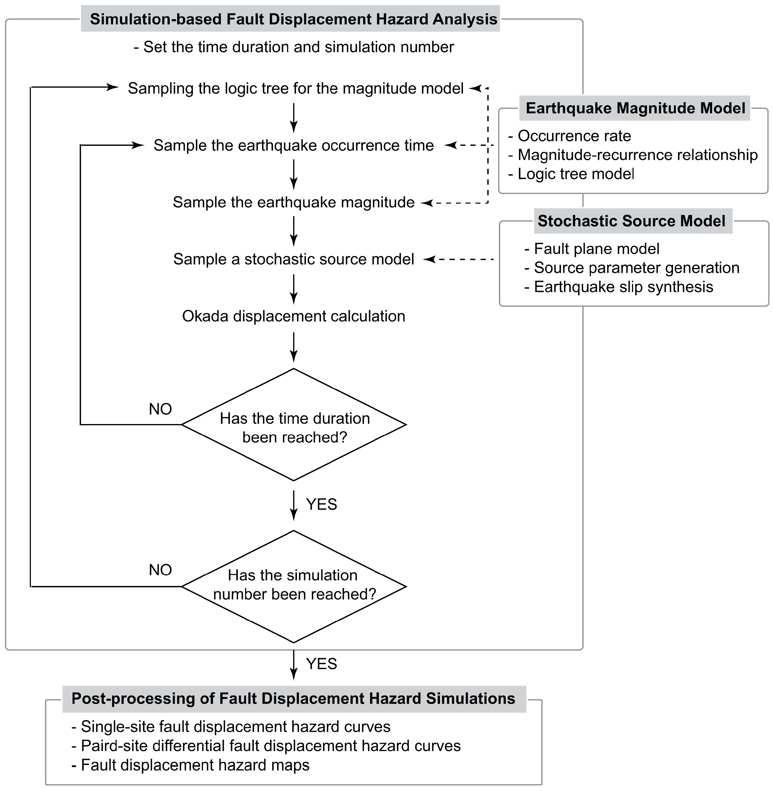
2.1. Methodology

In this section, a framework for prospective evaluation of the likelihood of surface fault displacement is presented. The rate of surface fault displacement D exceeding a given surface fault displacement d can be given by
ν D ( D d ) = λ M m i n P ( D d | s m , m ) f S M | M ( s m | m ) f M ( m ) d s m d m
where λ M m i n is the annual occurrence rate of earthquakes having magnitudes Mmin or larger, while fM is the conditional probability distribution of earthquake magnitude M above Mmin. fSM|M is the probability density function of a source model SM given M. P (Dd|sm,m) is the probability of exceeding a specified fault displacement given an earthquake source model SM and magnitude M.
Applying statistical prediction models of earthquake source parameters and synthesizing the heterogeneous earthquake slip can address the uncertainty associated with variable source characteristics. Okada equations are used to evaluate fault displacement functions for the simulated earthquake source models. The proposed approach based on Equation (1) is an integrated version of the two approaches [6] utilizing the stochastic source models and Okada equations to calculate surface fault displacement at a site of interest, instead of the empirical predictive relationship of surface fault displacement. It is important to emphasize that because Okada equations predict the spatial fault displacement distribution, rather than the occurrence and extent of actual surface fault rupture, no distinction between primary and distributed ruptures is made, unlike empirical fault displacement equations [12,13].
PFDHA, which employs stochastic source modeling and Okada equations, is applicable to an area with available seismological/geological information (see Section 2.2). From a computational perspective, Equation (1) can be implemented in Monte Carlo simulations. The first step of the evaluation is to specify earthquake scenarios with a range of earthquake magnitudes within a time duration of interest as well as earthquake occurrence model and magnitude distribution (i.e., λ M m i n and fM). To account for epistemic uncertainty of earthquake occurrence and magnitude models, a logic tree can be implemented (see Section 2.3). The second step is to specify a fault plane geometry (which may consist of multiple segments) and generate source parameter samples (e.g., fault length, fault width, mean slip, and maximum slip) from statistical scaling relationships [18]. Then, heterogenous earthquake slip distributions [19,20] are synthesized to generate various stochastic source models (see Section 2.4). A stochastic source model is a collection of earthquake slip values on the fault-rupture plane. In the third step, for each stochastic source model, three orthogonal displacement fields can be calculated using Okada equations (see Section 2.5). Finally, a fault displacement hazard curve νD(Dd) for a single site or a differential fault displacement hazard curve for paired sites can be obtained as a product of the assessment. The aforementioned procedure is summarized in Figure 1.

2.2. Target Fault Source: Leech River Valley Fault

2.2.1. Geological Setting

The LRVF is a prominent crustal fault cutting across southern Vancouver Island, which is known as the most earthquake-prone region in Canada [24,25]. There is structural and geomorphic evidence (e.g., mapped scarps, LiDAR elevation data with ~2 m horizontal by ~10 cm vertical resolutions, and bedrock and surficial field mapping), indicating that some strands of the LRVF have been active since the late Pleistocene. Recent studies indicate that the LRVF is a reverse fault zone with a north-dipping angle of 60° to 70° and a total length of 60 to 70 km [26]. The estimated slip rate is ≥0.2–0.3 mm/year for the Holocene and three earthquakes with surface rupture over the last 9000 years [25]. The slip rate was estimated by radiocarbon data for earthquake ages at specific trenches and fault displacement data based on stratigraphic offsets. Based on the length of the LRVF and the empirical relations [28], possible seismic events from the LRVF can be attributed to Mw6.9.
Figure 2a shows mapped scarps that have a nearly linear trace across topography along the LRVF based on [25]. Morell et al. [25] used LiDAR and field data to identify these geomorphic features (e.g., see Figure 2 of [25]) and concluded that the LRVF is active since the late Pleistocene. The topographic features originated from tectonic movements and exhibited extensive brittle faulting, excluding the assumptions of ice plucking or erosion of a bedrock foliation. These features were further supported by the observation of paleo-ice flow with the direction to the south, with a high angle to the orientation of the existing scarps. The linear shape of the scarps was another line of evidence that eliminated the possibility of landslides (identified with curvilinear heads) in forming these topographic features. Some of the fault strands indicated dip-slip motion on vertical or south-dipping high-angle faults, revealing a normal or reverse faulting mechanism.

2.2.2. Fault Plane Model

In the present study, a seismic source model was developed for the LRVF system based on the stochastic source modeling approach [22]. The geometry was determined based on [25,26], and rectangular finite fault sources were assumed on the fault-rupture plane of the LRVF. The total length of the LRVF is 70 km, and its width is set to 30 km with a dip angle of 70°. Figure 2b depicts spatial characteristics of the segmented rupture plane. It consists of 525 subfaults, each having a 2 km × 2 km dimension. The stochastic source approach accounts for the spatial uncertainty of the rupture size and location within the fault plane boundary, which is important due to the proximity of the LRVF to Victoria. The earthquake magnitude model [29], which is based on the seismic moment rate balancing, was adopted (see Section 2.3). The wider fault zone assumed for the LRVF can contribute to the uncertainty in rupture geometry and its position. It leads to an increase in the frequency of large-magnitude earthquakes but decreases the frequency of moderate-to-large earthquakes to conserve the total seismic moment in the area. Presenting the details of the seismic hazard model in southwestern British Columbia is avoided, as more information can be found in [27]. A complete seismic hazard assessment for other sources is provided in the 2020 Geological Survey of Canada model [26].

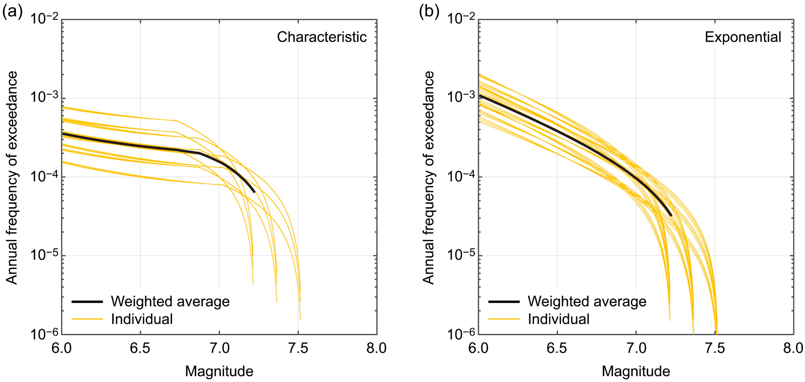
2.3. Earthquake Magnitude Model

Two popular approaches for describing the magnitude distribution of a seismic source are the truncated exponential model and the characteristic earthquake model [29]. Although the latter is generally regarded to be suitable for a fault source, recent PSHA studies from California [30] and New Zealand [31] suggested that the model cannot be clearly identified as superior to the truncated exponential model, and thus, both models are viable alternatives in conducting seismic hazard assessments. The same approach was taken by [26,27] in conducting the fault-source-based PSHA for the LRVF.
The two magnitude models produce the same seismic moment release, which is controlled by the slip rate Sr of a fault zone with an area Af and with the shear modulus μ (i.e., seismic moment release = µ SrAf). The probability density function of the characteristic magnitude model is given by [29,32]
f M ( m ) = 0 for m < M m i n β exp ( β ( m M m i n ) ) ( 1 + C ) [ 1 exp ( β ( M m a x M m i n Δ m 2 ) ) ] for M m i n m < M m a x Δ m 2 β exp ( β ( M m a x M m i n Δ m 1 Δ m 2 ) ) ( 1 + C ) [ 1 exp ( β ( M m a x M m i n Δ m 2 ) ) ] for M m a x Δ m 2 m M m a x 0 for m > M m a x
where the constant C is expressed as
C = β exp ( β ( M m a x M m i n Δ m 1 Δ m 2 ) ) 1 exp ( β ( M m a x M m i n Δ m 2 ) ) Δ m 2 .
In Equations (2) and (3), β = blog10, with b-value of the Gutenberg–Richter relationship (i.e., exponential magnitude distribution); Mmin and Mmax are the minimum magnitude and maximum magnitude for the fault source, respectively; ∆m1 and ∆m2 are the magnitude intervals used to specify the probability density values for the exponential distribution part (magnitude range between Mmin and Mmax – ∆m2) and the uniform distribution part (magnitude range between Mmax – ∆m2 and Mmax). The truncated exponential magnitude model can be achieved by setting ∆m2 = 0 (i.e., C = 0) in the above equations.
With scarce information to constrain the activity of the LRVF, it is important to consider alternative magnitude models [26]. For this purpose, the same logic-tree model for the magnitude distribution of the LRVF, considered by [27], was adopted. The logic-tree magnitude model for the LRVF incorporates the truncated exponential and characteristic models with equal weights. For each magnitude model, three key parameters—namely, slip rate (Sr), b-value (equivalent to β value), and Mmax—are varied by considering three possible values with different weights. The parameter values and weights are listed in Table 1. According to sensitivity analyses conducted by [27], one of the most influential parameters is the slip rate. The range of the variability of Sr considered in Table 1 (i.e., 0.15–0.35 mm/year) is consistent with [25] (i.e., 0.2–0.3 mm/year). Other relevant parameters are set as follows: μ = 35 GPa; Af is calculated based on the fault geometry shown in Figure 2b; Mmin = 6.0; ∆m1 = 1.0; ∆m2 = 0.5. These values are consistent with those reported in [26]; details can be found in [27].
Figure 3 illustrates 27 variations in the magnitude–recurrence relationships for the LRVF associated with the characteristic and truncated exponential models; the weighted average relationship of the curves is also included in each figure panel. As shown in Figure 3a, there are kinks in the recurrence curves of the characteristic models, while the recurrence curves of the exponential models decay smoothly (Figure 3b). Furthermore, the characteristic models result in lower frequencies of earthquake occurrence than the exponential models in the lower magnitude range due to the distribution of the seismic moment in larger magnitude earthquakes. These magnitude distributions (i.e., 54 cases) were used in PFDHA and are implemented in the earthquake magnitude modeling component of the flowchart shown in Figure 1 (see also Equation (1)). By adopting a simulation-based seismic hazard method, for a given scenario, earthquake magnitudes and occurrence times can be sampled based on the logic tree branches. Then, the earthquake occurrence rate ( λ M m i n ) and probability density function of earthquakes (fM) were calculated.

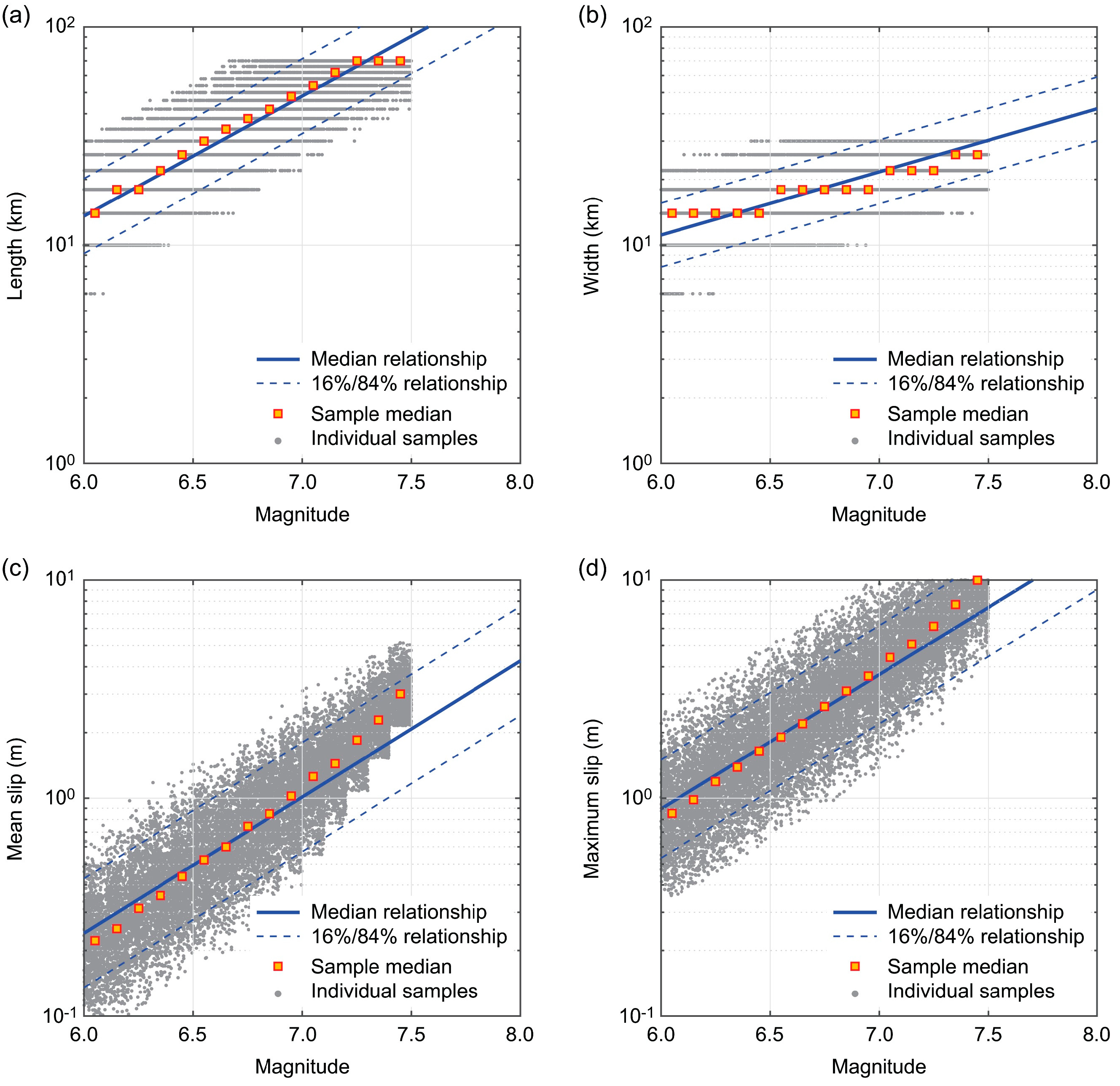
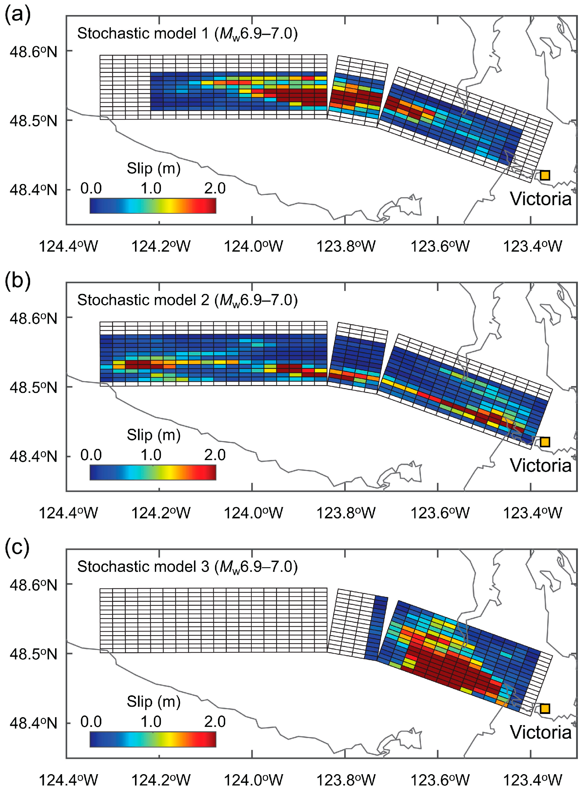
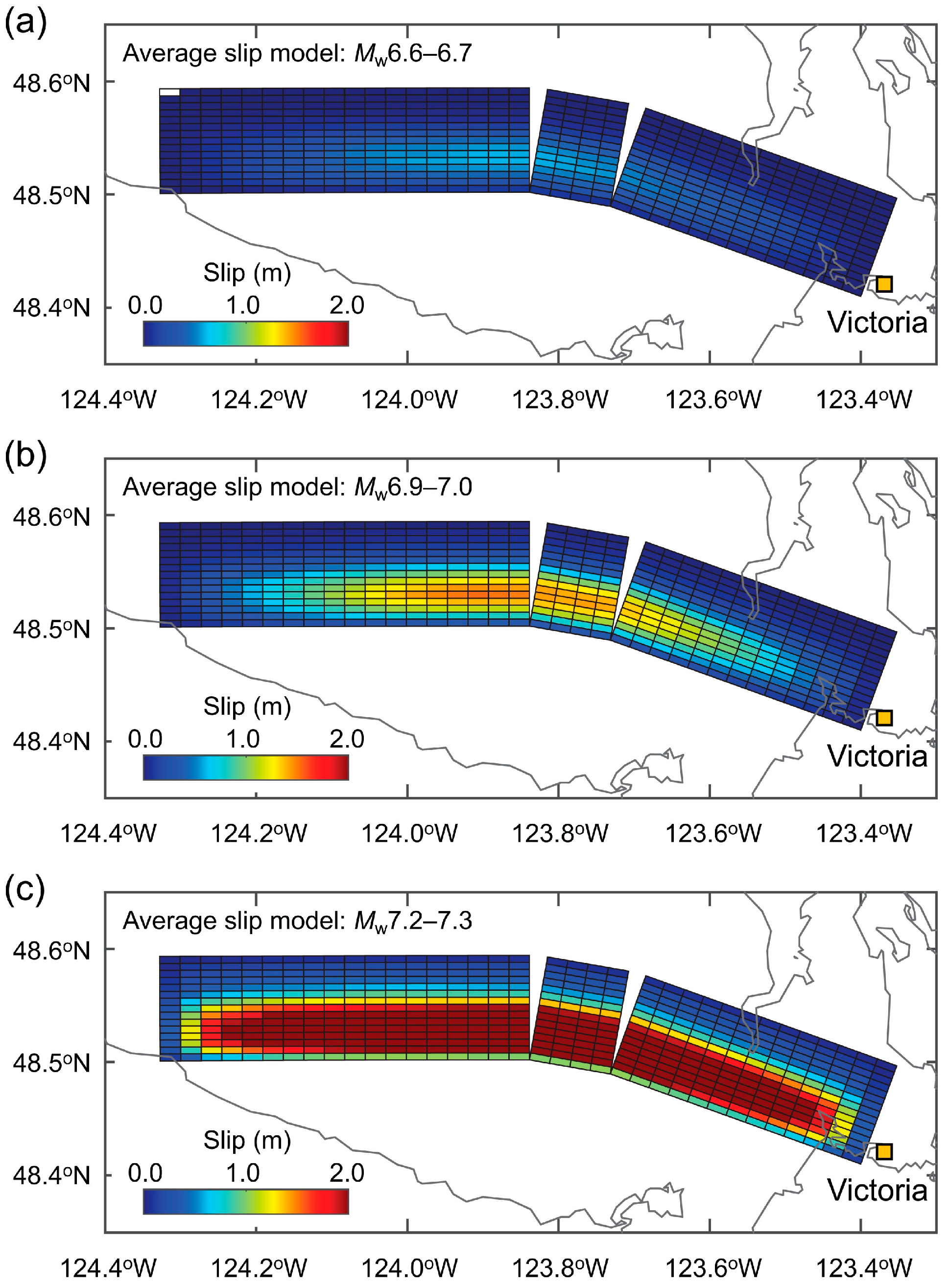
2.4. Stochastic Source Model

Fault displacement hazard assessment requires a fault-rupture model for the region of interest to specify an earthquake scenario. The defined fault plane (shown in Figure 2b) is discretized into multiple subfaults. Subsequently, eight source parameters were generated to synthesize stochastic source models with heterogeneous slip distributions. The eight parameters, listed in Table 2, are obtained from the statistical scaling relationships [18]; the details of the equations can be found in [18] and are not repeated here. It is important to point out that these earthquake source parameters are statistically dependent, and this dependency is reflected by sampling these parameters with a proper correlation structure [18].
The two geometrical parameters L and W define the fault-rupture area, whereas the earthquake slip parameters Da, Dm, and λBC determine the marginal distribution of the earthquake slip on the fault-rupture plane. In particular, the Box–Cox transformation with λBC is used to achieve a desirable right-skewed feature of the slip marginal distribution [20]. To characterize the spatial complexity of earthquake slip, spectral synthesis of random slip fields adopts an anisotropic 2D von Kármán wavenumber spectrum, with its amplitude spectrum being parametrized by along-strike correlation length CL, along-dip correlation length CW, and Hurst number H, and its phase being randomly distributed between 0 and 2π [19]. Once a random earthquake slip is generated for a given fault geometry, the slip distribution is converted using the Box–Cox transformation and its associated parameter (λBC) to achieve a realistic heavier right-tail distribution. The obtained distribution is adjusted by the mean and maximum slips (Da and Dm), and the corresponding seismic moment is calculated for the generated source model with consistent values of L, W, and Da. The candidate stochastic source model is accepted if it produces the seismic moment within the target range (e.g., Mw6.5 and Mw6.6); otherwise, the procedure is repeated [18].
Figure 4 shows the sampled source parameters for the fault length (L), fault width (W), mean slip (Da), and maximum slip (Dmax). The magnitude range between 6 and 7.5 is considered and divided into 15 bins with 0.1 widths. The maximum magnitude of Mw7.5 corresponds to the upper limit of the moment magnitude for the fault plane shown in Figure 2b and is selected based on the fault area scaling relationship [33] by taking a mean plus 1.5 times the standard deviation. For each magnitude bin, 1000 stochastic source models are generated. The discrete characteristics of the fault length and width shown in Figure 4a,b, respectively, are because the fault dimensions can only take the odd multiples of subfault sizes (= 2 km), i.e., 2, 6, 10, etc. This requirement of the odd multiples of the subfault size stems from the generation of wavenumber vectors specified at the lower and upper boundary wavenumbers and at zero wavenumbers in the earthquake slip synthesis method proposed by [19]. In the simulated samples of the fault dimensions, the effects of saturation of the fault area can be observed (i.e., the maximum dimensions are limited to 70 km and 30 km for the fault length and width, respectively). Consequently, to satisfy the target seismic moment for large earthquake scenarios (e.g., Mw greater than 7.1), the mean and maximum slips start to deviate upward from the mean scaling relationships. On the other hand, for small to moderate earthquake scenarios (e.g., Mw smaller than 7.1), simulated stochastic source models have representative characteristics similar to the empirical scaling relationships.
To illustrate earthquake slip distributions of the stochastic source models, Figure 5 depicts three realizations of the 1000 simulated source models for the magnitude bin Mw6.9–7.0. The figure shows that the simulated source models can have smaller geometry than the defined source zone; hence, they can be floated within the fault zone. Additionally, the slip distributions vary according to the scaling relationships and realizations of the earthquake slip synthesis. Some models have large slip values that are concentrated near the center of the fault-rupture plane, which is not densely populated (Figure 5a), while others have large slip concentrations that are relatively close to populated areas near Victoria (Figure 5b,c). In short, by using the 1000 stochastic source models, a wide range of possible earthquake ruptures for the specified earthquake magnitude can be captured.
Moreover, to illustrate the overall earthquake slip characteristics of the stochastic source models, Figure 6 shows the averages of all 1000 simulated source models for three magnitude scenarios. The three average source models shown in this figure reveal that the overall trend of the slip values changes with earthquake magnitude. The scenarios with larger magnitudes lead to higher average slip values of the generated source models and fill the wider area of the fault plane, as seen in Figure 4.

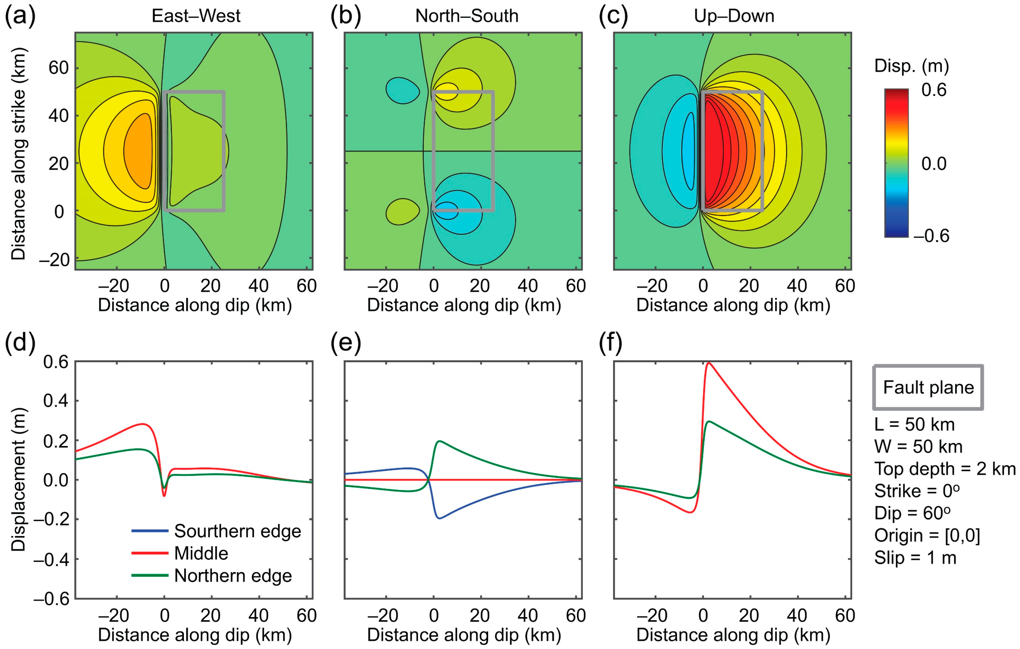
2.5. Fault Displacement Calculation

For the simulated slip distributions (Section 2.4), surface fault displacements are calculated using Okada equations for three transitional directions (i.e., east–west, north–south, and up–down). A hypothetical fault (Figure 7) is used to explain the calculation of surface fault displacements. The geometry of the hypothesized fault is 50 km long and 50 km wide; the top of the fault plane is 2 km deep with a 0° strike and 60° dip, having a reverse faulting mechanism (90° rake). A 1 m slip is assumed for this hypothetical fault rupture. Figure 7a–c show the spatial distributions of displacements for all three components of the fault plane with a unit slip. Figure 7d–f illustrate the three cross-sectional profiles (center and two edges of the rupture plane) of the displacements associated with each direction. In the east–west direction, there is a larger displacement in the footwall in comparison with the hanging wall, which is expected for a reverse faulting mechanism. In the north–south direction, there is a displacement at the rupture boundaries, which can be attributed to the bulging of the hanging wall fault due to the vertical displacement. The surface displacement of ∼0.6 m is calculated for the up–down direction with the maximum upward displacement in the hanging wall side of the fault plane and downward displacement in the footwall side of the fault plane. The displacement values decrease with increasing distance from the fault in all directions.
In computing the total surface displacement due to a fault movement with heterogeneous slip distribution (e.g., Figure 5), the fault displacements of each subfault can be evaluated using Okada equations (as demonstrated in Figure 7), and then their individual effects are summed up for all subfaults. For each stochastic source model generated in Section 2.4, the same procedure can be performed, and this model component can be implemented as part of the PFDHA framework shown in Figure 1. It is important to point out that the geometrical parameters, such as rake and dip, are uncertain. For instance, there may be conflicting field observations to suggest different faulting mechanisms. This uncertainty can be incorporated into the PFDHA framework by defining multiple fault planes (Section 2.2.2) and implementing them in a logic tree.

3. Probabilistic Fault Displacement Hazard Analysis of the Leech River Valley Fault

A simulation-based fault displacement hazard assessment (Figure 1) was carried out for the LRVF. In presenting PFDHA results, we mainly focus on horizontal and vertical surface fault displacements. The horizontal displacements are the vector sum of the east–west and north–south components. The simulation setup for PFDHA and the key aspects of the studied sites are presented in Section 3.1. In Section 3.2, the evaluated fault displacement hazards for the single and paired sites (i.e., differential fault displacements) are presented as hazard curves in terms of horizontal and vertical displacements. Finally, hazard maps for the critical scenarios are developed in Section 3.3 by focusing on differential fault displacements of the given paired sites.

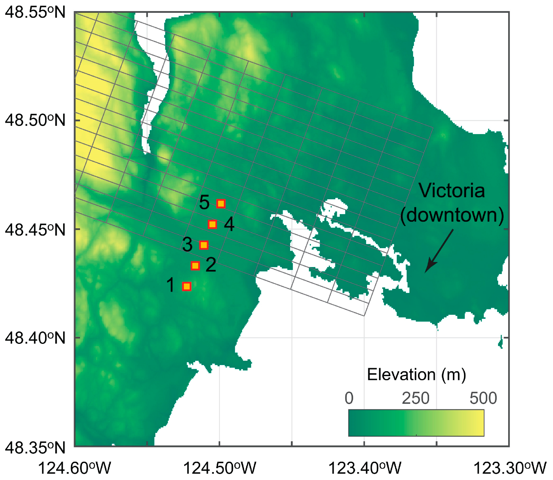
3.1. Simulation Setup and Site Selection

PFDHA was conducted by characterizing the possible earthquake ruptures of the LRVF (Section 2.2) based on the magnitude recurrence relationships (Section 2.3) and by assigning stochastic source models to these scenarios (Section 2.4). For each combination of earthquake scenario and stochastic source, fault displacements were evaluated using Okada equations (Section 2.5). For illustration, five hypothetical sites in Langford, British Columbia, with an inter-site distance of 1 km were selected (Figure 8). Sites 1 and 2 are on the footwall side of the LRVF, whereas Sites 3 to 5 are on the hanging wall side of the LRVF. Different magnitude models and model parameters for the magnitude–recurrence relationships were considered using the logic tree (Table 1 and Figure 3). To develop the stochastic source models, the source region of the LRVF (Figure 2b), which is large enough to include stochastic sources with various magnitudes and sizes, was defined and discretized into 2 × 2 km subfaults. The earthquake source parameters (Figure 4) and corresponding random slip fields (Figure 5 and Figure 6) were simulated, and subsequently, fault displacements were computed at the sites of interest (Figure 7). The duration of the simulation was set to 10 million years, noting that the mean recurrence period of the LRVF was relatively long (typically, 1000 years for Mw6+ events; Figure 3).

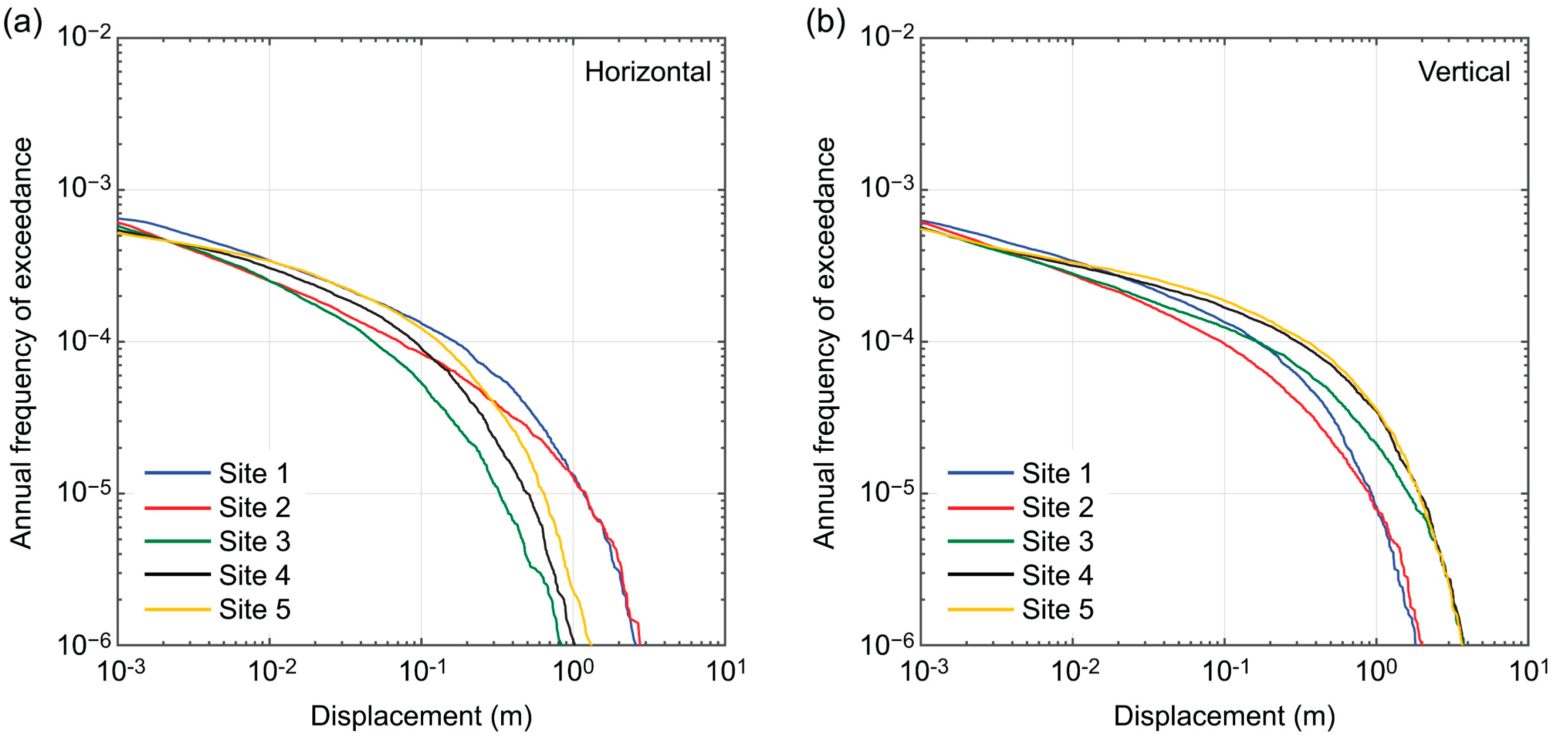
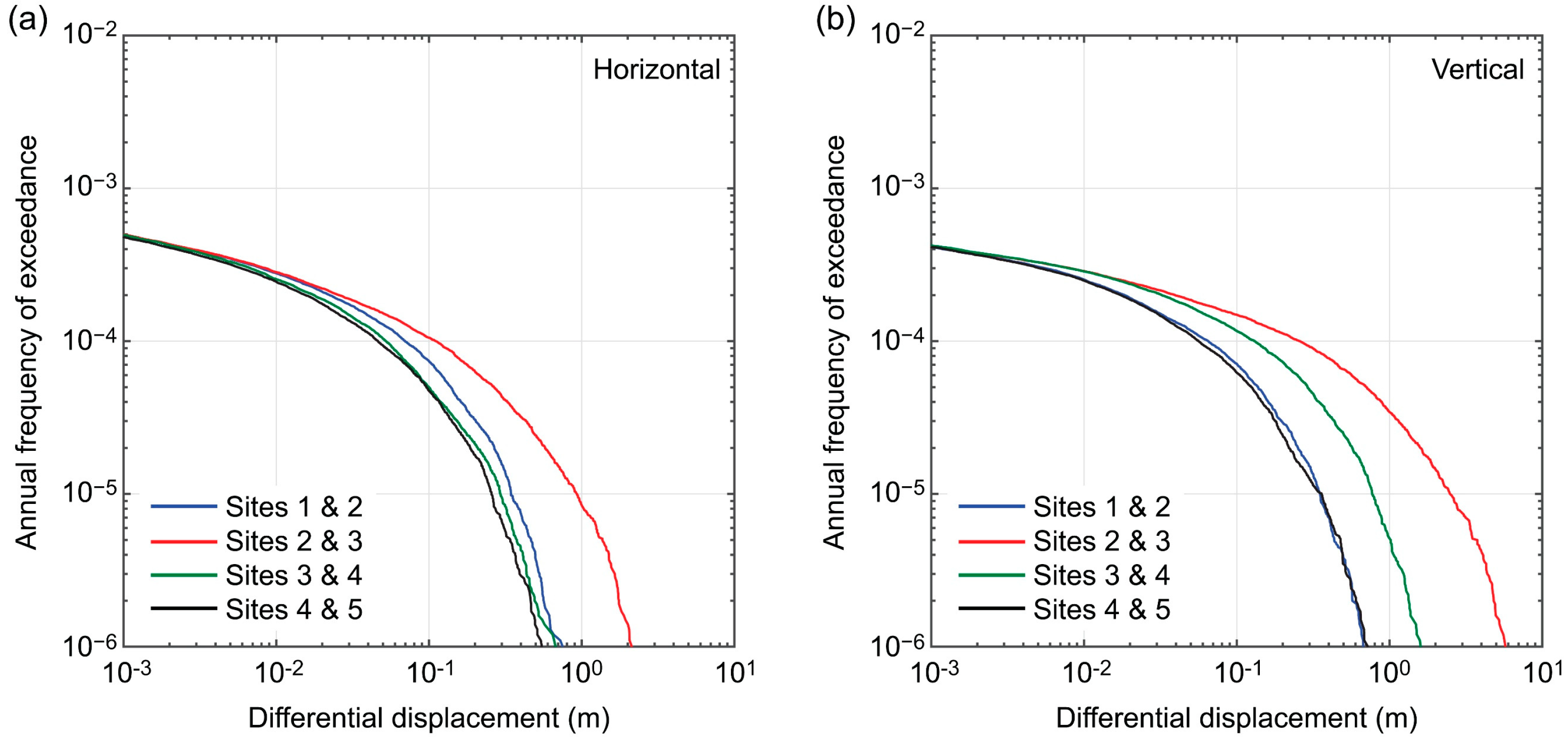
3.2. Fault Displacement Hazard Curves

Fault displacement hazard curves for individual and paired sites were developed. Figure 9 depicts the results of PFDHA for the horizontal displacement (Figure 9a) and vertical displacement (Figure 9b) of Sites 1 to 5. On the footwall side (Sites 1 and 2), horizontal displacements are more dominant than vertical displacements; by contrast, on the hanging wall side (Sites 3 to 5), vertical displacements are greater than horizontal displacements. The observed results are caused by reverse faulting mechanisms of the LRVF ruptures and are consistent with the illustrative Okada calculations shown in Figure 7. For rare cases (annual frequency of 10−4), some large displacements exceeding 0.1 m (up to 0.5 m vertical uplift at hanging wall sites) are likely to occur. Relatively low fault displacement hazards in Langford are mainly attributed to a low frequency of major earthquake ruptures of the LRVF.
Figure 10 shows the differential fault displacement hazard curves for paired sites. The differential displacement hazards for Sites 2 and 3 are significantly greater than other paired sites. This is because Site 2 is on the footwall side of the fault plane, while Site 3 is on the hanging wall side of the fault plane. At the annual frequency of 10−4, for instance, the differential vertical displacement of 0.5 m or greater is possible for Sites 2 and 3. The differential displacements tend to become large when the two sites experience different relative fault movements. For the reverse faulting case, vertical differential displacements are more critical than horizontal differential displacements. However, different situations would arise for different faulting mechanisms (e.g., for strike-slip events, differential horizontal displacements become dominant for two sites across the fault strike). Importantly, the results from the differential fault displacement hazard curves can be used for further analyses of engineered structures, such as bridges and pipelines, to assess their structural integrity and seismic performance under extreme loading conditions.
Similar to the PSHA disaggregation, hazard contributions from different earthquake scenarios can be evaluated using the detailed outputs from PFDHA. Figure 11a,b show the histograms of earthquake magnitudes of LRVF ruptures that produce the differential displacements larger than 0.5 m and 1.0 m, respectively, for Sites 2 and 3. The dominant earthquake scenarios are from Mw7.0+ events for both differential displacement cases. With the increase in the displacement threshold, larger earthquake events tend to contribute more to the differential displacement hazards, which is expected.

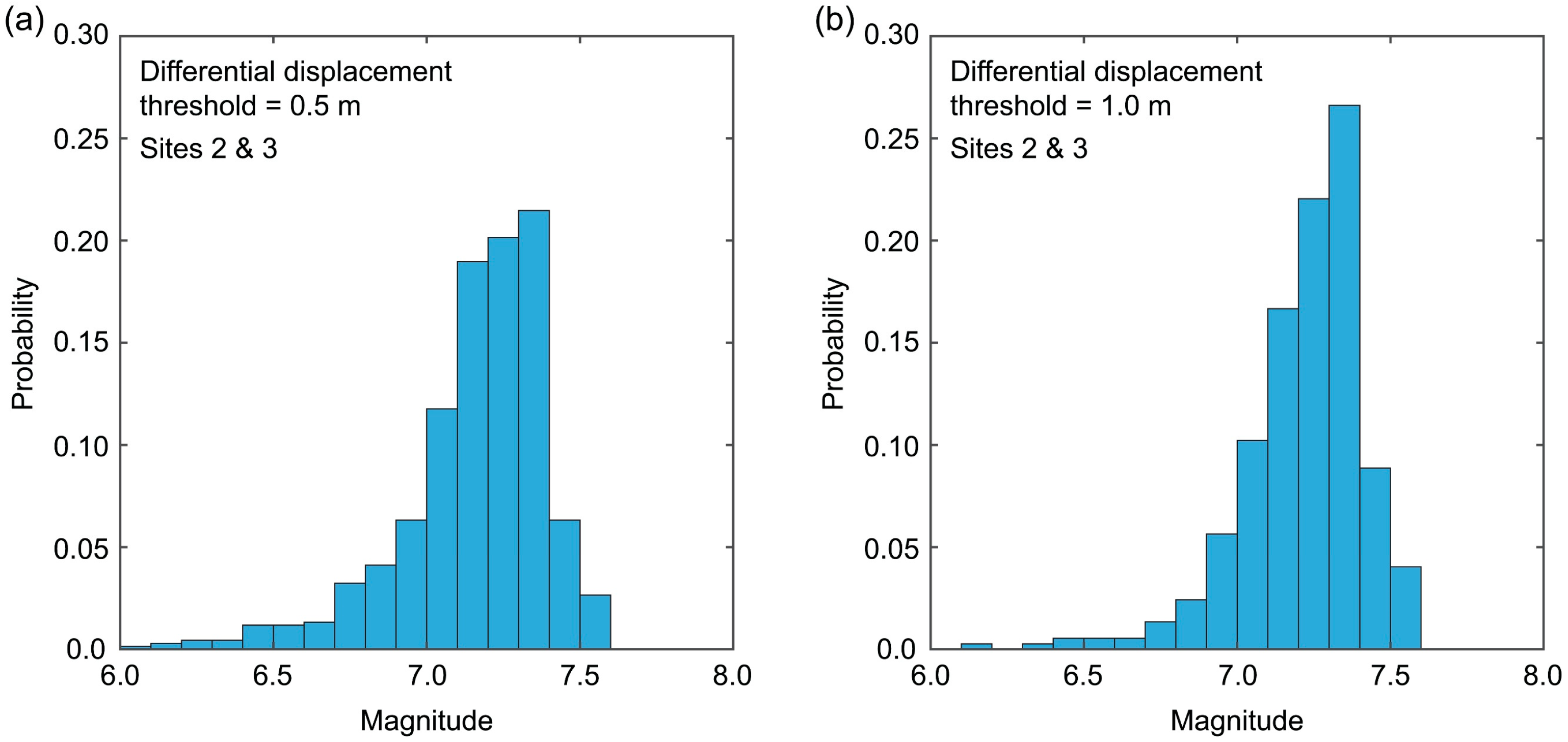
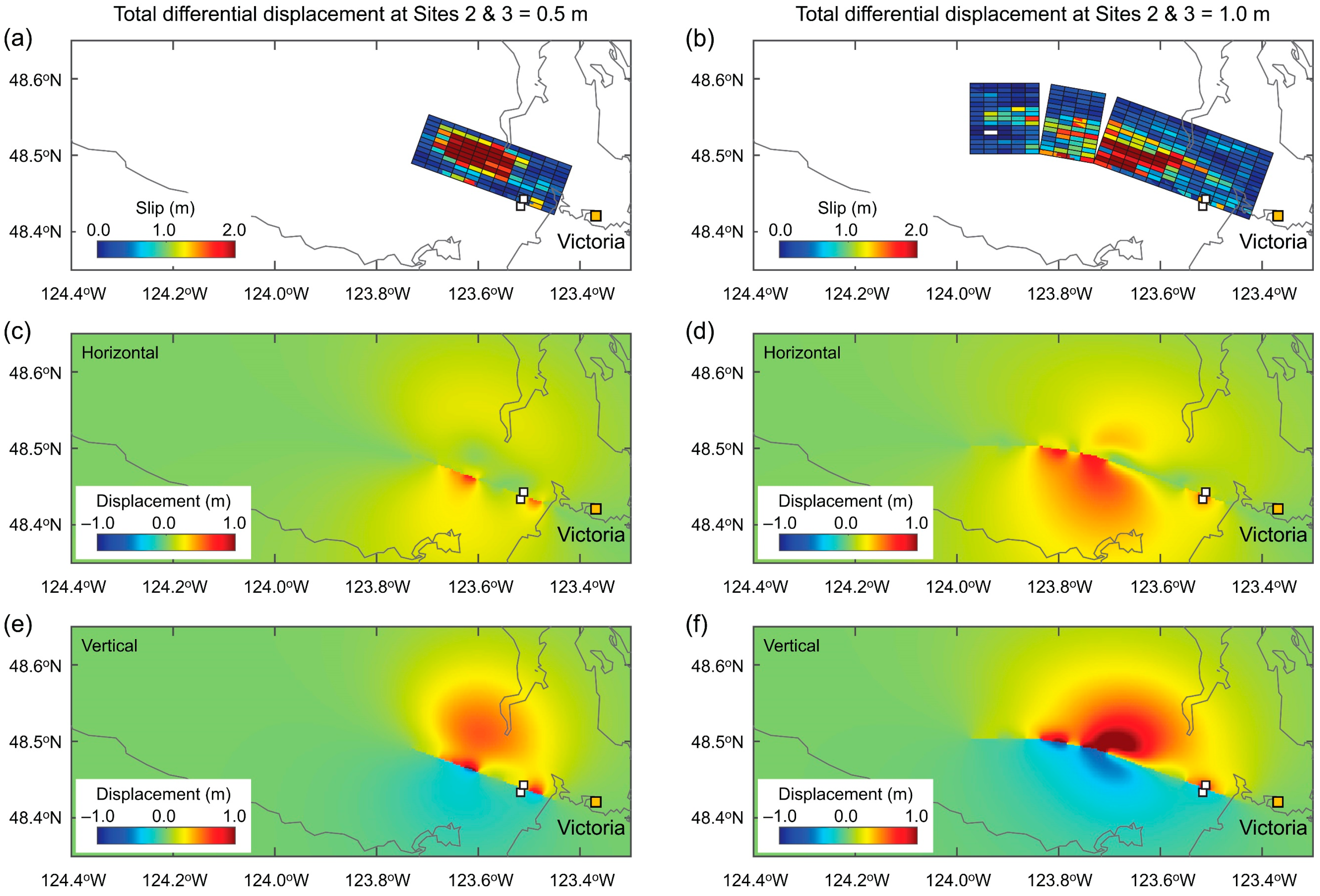
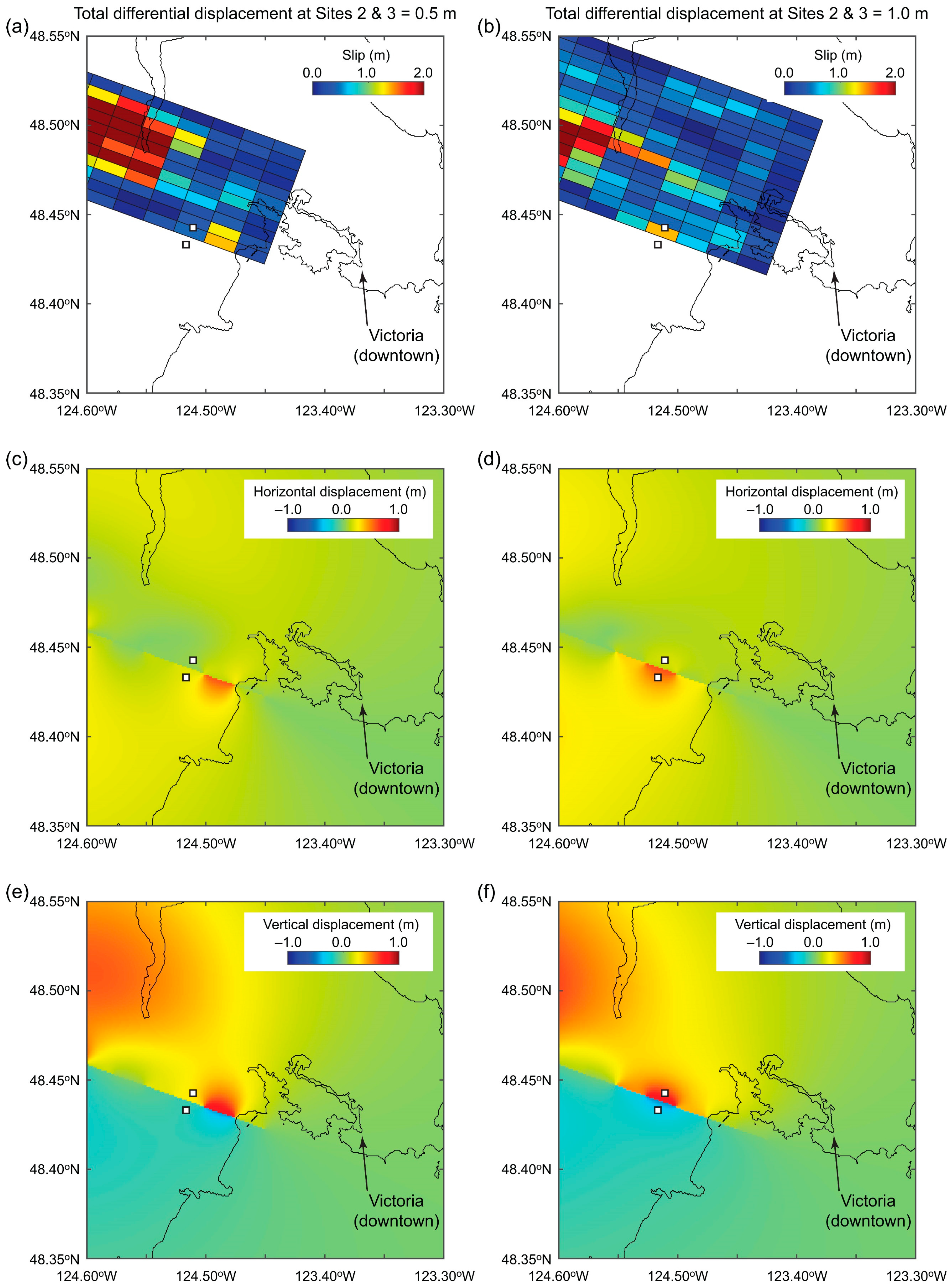
3.3. Fault Displacement Hazard Maps for Critical Scenarios

As one of the useful outputs from the simulation-based PFDHA, critical scenario hazard maps for fault displacement can be developed. It is noted that critical hazard maps are different from so-called uniform hazard maps that are used for national seismic hazard mapping. The main difference between the two types of hazard maps is that the critical scenario hazard map corresponds to a specific earthquake rupture scenario, which results in a specified hazard value (or associated with a specified annual frequency of exceedance) and, thus, preserves the spatial dependence of the calculated hazard values at different locations, while the uniform hazard map is developed by evaluating the site-specific hazard at individual locations independently.
To demonstrate the development of the critical scenario hazard maps for fault displacement, two scenarios of differential displacements of 0.5 m and 1 m for Sites 2 and 3 were selected. These scenarios correspond to 6.8 × 10⁻⁵ and 3.8 × 10⁻⁵ annual frequency of exceedance. Figure 12a,b illustrate the regional views of the slip distribution for two selected source models. Figure 12c,d show the horizontal fault displacement hazard maps, whereas Figure 12e,f show the vertical displacement hazard maps. Figure 13 shows the local views of Figure 12 near Sites 2 and 3. As shown in Figure 12c (Figure 13c), there is a larger horizontal displacement on the footwall side of the fault plane (Site 2) than on the hanging wall side of the fault plane (Site 3). This is reversed in the case of the vertical displacement and larger surface displacement appears on the hanging wall side of the fault plane, as shown in Figure 12e (Figure 13e). With the increase in the fault displacement hazard threshold, the extent of fault displacements tends to be more extensive (as expected). Although the frequencies of the hazard for 0.5 m and 1 m fault displacements in the LRVF are low, such probable rupture scenarios are relevant and should be considered because of the potential consequences that can be caused by the failures of critical infrastructure in Victoria and the surrounding region. These critical fault displacement hazard maps are useful for emergency management purposes.

4. Conclusions

4.1. Summary and Key Findings

This study proposed a new approach to performing probabilistic fault displacement hazard analysis (PFDHA) by combining stochastic source modeling and Okada equations. The method was applied to the Leech River Valley Fault (LRVF) to evaluate the potential fault displacement hazard due to an earthquake rupture. The outputs of the PFDHA for the LRVF were obtained as fault displacement hazard curves at single sites, as well as differential fault displacement hazard curves at paired sites. From the case study for the five sites in Langford, British Columbia, the following specific conclusions can be drawn:
  • The results for the LRVF region indicate that a surface vertical displacement of 0.5 m is possible at a low annual frequency of exceedance (annual frequency of 10−4). The low chance of a major fault displacement hazard is attributed to the low seismic activity of the LRVF (i.e., mean recurrence periods of moderate-size earthquakes are around 1000 years). Although the probability is low, the consideration of the surface fault displacement of the LRVF is important as it may affect local critical infrastructures widely and simultaneously.
  • The differential fault displacement hazards for two sites that are located across the fault strike (i.e., one site is on the footwall side of the fault, while the other site is on the hanging wall side of the fault) are significantly greater than other paired sites that are located on the same side of the fault. For critical linear infrastructure crossing the fault trace, assessing the structural integrity against possible differential fault displacement hazards is important.

4.2. Perspectives

For future studies, two research directions can be suggested. Firstly, it is important to apply the fault displacement method based on the stochastic source modeling and Okada equations to many more historical events from retrospective perspectives [22,23], and their accuracy should be compared against all types of available observations. In this regard, the development of extensive fault displacement databases is essential [13,16,17]. The prediction errors of the fault displacement method can be quantified and can be incorporated into PFDHA. Secondly, more rigorous characterization of epistemic uncertainty related to earthquake sources can be investigated, such as consideration of multiple fault planes in the logic tree and consideration of different earthquake source scaling relationships. These refinements will improve the comprehensiveness of uncertainty quantification associated with fault displacement hazard analysis. Such approaches will open new avenues for seismic performance evaluations of critical facilities and infrastructure subject to multi-hazard actions (e.g., transient shaking and permanent fault displacement).

Author Contributions

K.G. developed the research plan and computer codes, and carried out the analyses. P.S. contributed to the writing of this paper and checked the accuracy of the analyses. All authors have read and agreed to the published version of the manuscript.

Funding

This study is funded by the Canada Research Chair program (950–232015) and the NSERC Discovery Grant (RGPIN-2019–05898). The APC is funded by the same funding programs.

Data Availability Statement

All information is described in the maintext.

Conflicts of Interest

The author declares no conflict of interest.

References

  1. Yang, S.; Mavroeidis, G.P. Bridges crossing fault rupture zones: A review. Soil Dyn. Earthq. Eng. 2018, 113, 545–571. [Google Scholar] [CrossRef]
  2. Katona, T.J.; Tóth, L.; Győri, E. Fault displacement hazard analysis based on probabilistic seismic hazard analysis for specific nuclear sites. Appl. Sci. 2021, 11, 7162. [Google Scholar] [CrossRef]
  3. Valentini, A.; Fukushima, Y.; Contri, P.; Ono, M.; Sakai, T.; Thompson, S.C.; Viallet, E.; Annaka, T.; Chen, R.; Moss, R.E.S. Probabilistic fault displacement hazard assessment (PFDHA) for nuclear installations according to IAEA safety standards. Bull. Seismol. Soc. Am. 2021, 115, 2661–2672. [Google Scholar] [CrossRef]
  4. Ni, P.; Mangalathu, S.; Yi, Y. Fragility analysis of continuous pipelines subjected to transverse permanent ground deformation. Soils Found. 2018, 58, 1400–1413. [Google Scholar] [CrossRef]
  5. Garcia, F.E.; Bray, J.D. Discrete element analysis of earthquake surface fault rupture through layered media. Soil Dyn. Earthq. Eng. 2022, 152, 107021. [Google Scholar] [CrossRef]
  6. Youngs, R.R.; Arabasz, W.J.; Anderson, R.E.; Ramelli, A.R.; Ake, J.P.; Slemmons, D.B.; McCalpin, J.P.; Doser, D.I.; Fridrich, C.J.; Swan III, F.H.; et al. A methodology for probabilistic fault displacement hazard analysis (PFDHA). Earthq. Spectra 2003, 19, 191–219. [Google Scholar] [CrossRef]
  7. Stepp, J.C. Probabilistic seismic hazard analyses for fault displacement and ground motions at Yucca Mountain, Nevada. Earthq. Spectra 2001, 17, 113–151. [Google Scholar] [CrossRef]
  8. Cornell, C.A. Engineering seismic risk analysis. Bull. Seismol. Soc. Am. 1968, 58, 1583–1606. [Google Scholar] [CrossRef]
  9. Baker, J.W.; Bradley, B.A.; Stafford, P.J. Seismic Hazard and Risk Analysis; Cambridge University Press: Cambridge, UK, 2021; p. 600. [Google Scholar]
  10. Takao, M.; Tsuchiyama, J.; Annaka, T.; Kurita, T. Application of probabilistic fault displacement hazard analysis in Japan. J. Jpn. Assoc. Earthq. Eng. 2013, 13, 17–36. [Google Scholar] [CrossRef]
  11. Wesnousky, S.G. Displacement and geometrical characteristics of earthquake surface ruptures: Issues and implications for seismic hazard analysis and the earthquake rupture process. Bull. Seismol. Soc. Am. 2008, 98, 1609–1632. [Google Scholar] [CrossRef]
  12. Petersen, M.D.; Dawson, T.E.; Chen, R.; Cao, T.; Wills, C.J.; Schwartz, D.P.; Frankel, A.D. Fault displacement hazard for strike-slip faults. Bull. Seismol. Soc. Am. 2011, 101, 805–825. [Google Scholar] [CrossRef] [Green Version]
  13. Nurminen, F.; Boncio, P.; Visini, F.; Pace, B.; Valentini, A.; Baize, S.; Scotti, O. Probability of Occurrence and displacement regression of distributed surface rupturing for reverse earthquakes. Front. Earth Sci. 2020, 8, 581605. [Google Scholar] [CrossRef]
  14. Moss, R.E.; Ross, Z.E. Probabilistic fault displacement hazard analysis for reverse faults. Bull. Seismol. Soc. Am. 2011, 101, 1542–1553. [Google Scholar] [CrossRef]
  15. Lavrentiadis, G.; Abrahamson, N. Generation of surface-slip profiles in the wavenumber domain. Bull. Seismol. Soc. Am. 2019, 109, 888–907. [Google Scholar] [CrossRef]
  16. Baize, S.; Nurminen, F.; Sarmiento, A.; Dawson, T.; Takao, M.; Scotti, O.; Azuma, T.; Boncio, P.; Champenois, J.; Cinti, F.R.; et al. A worldwide and unified database of surface ruptures (SURE) for fault displacement hazard analyses. Seismol. Res. Lett. 2020, 91, 499–520. [Google Scholar] [CrossRef] [Green Version]
  17. Sarmiento, A.; Madugo, D.; Bozorgnia, Y.; Shen, A.; Mazzoni, S.; Lavrentiadis, G.; Dawson, T.; Madugo, C.; Kottke, A.; Thompson, S.; et al. Fault Displacement Hazard Initiative Database; UCLA Natural Hazards Risk and Resiliency Research Center: Los Angeles, CA, USA, 2021. [Google Scholar] [CrossRef]
  18. Goda, K.; Yasuda, T.; Mori, N.; Maruyama, T. New scaling relationships of earthquake source parameters for stochastic tsunami simulation. Coast. Eng. J. 2016, 58, 1650010. [Google Scholar] [CrossRef] [Green Version]
  19. Mai, P.M.; Beroza, G.C. A spatial random field model to characterize complexity in earthquake slip. J. Geophys. Res. Solid Earth 2002, 107, ESE-10. [Google Scholar] [CrossRef]
  20. Goda, K.; Mai, P.M.; Yasuda, T.; Mori, N. Sensitivity of tsunami wave profiles and inundation simulations to earthquake slip and fault geometry for the 2011 Tohoku earthquake. Earth Planets Space 2014, 66, 105. [Google Scholar] [CrossRef] [Green Version]
  21. Okada, Y. Surface deformation due to shear and tensile faults in a half-space. Bull. Seismol. Soc. Am. 1985, 75, 1135–1154. [Google Scholar] [CrossRef]
  22. Goda, K. Potential fault displacement hazard assessment using stochastic source models: A retrospective evaluation for the 1999 Hector Mine earthquake. GeoHazards 2021, 2, 22. [Google Scholar] [CrossRef]
  23. Goda, K. Probabilistic characterization of seismic ground deformation due to tectonic fault movements. Soil Dyn. Earthq. Eng. 2017, 100, 316–329. [Google Scholar] [CrossRef] [Green Version]
  24. Li, G.; Liu, Y.; Regalla, C.; Morell, K.D. Seismicity relocation and fault structure near the Leech River fault zone, southern Vancouver Island. J. Geophys. Res. Solid Earth 2018, 123, 2841–2855. [Google Scholar] [CrossRef] [Green Version]
  25. Morell, K.D.; Regalla, C.; Amos, C.; Bennett, S.; Leonard, L.J.; Graham, A.; Reedy, T.; Levson, V.; Telka, A. Holocene surface rupture history of an active forearc fault redefines seismic hazard in southwestern British Columbia, Canada. Geophys. Res. Lett. 2018, 45, 11605–11611. [Google Scholar] [CrossRef]
  26. Halchuk, S.; Allen, T.I.; Adams, J.; Onur, T. Contribution of the Leech River Valley-Devil’s Mountain Fault system to seismic hazard in Victoria, British Columbia. In Proceedings of the 12th Canadian Conference on Earthquake Engineering 2019, Quebec City, QC, Canada, 17–20 June 2019. [Google Scholar]
  27. Goda, K.; Sharipov, A. Fault-source-based probabilistic seismic hazard and risk analysis for Victoria, British Columbia, Canada: A case of the Leech River Valley Fault and Devil’s Mountain Fault system. Sustainability 2021, 13, 1440. [Google Scholar] [CrossRef]
  28. Wells, D.L.; Coppersmithn, K.J. New empirical relationships among magnitude, rupture length, rupture width, rupture area, and surface displacement. Bull. Seismol. Soc. Am. 1994, 84, 974–1002. [Google Scholar] [CrossRef]
  29. Youngs, R.R.; Coppersmith, K.J. Implications of fault slip rates and earthquake recurrence models to probabilistic seismic hazard estimates. Bull. Seismol. Soc. Am. 1985, 75, 939–964. [Google Scholar] [CrossRef]
  30. Page, M.; Felzer, K. Southern San Andreas Fault seismicity is consistent with the Gutenberg–Richter magnitude–frequency distribution. Bull. Seismol. Soc. Am. 2015, 105, 2070–2080. [Google Scholar] [CrossRef]
  31. Stirling, M.; Gerstenberger, M. Applicability of the Gutenberg–Richter relation for major active faults in New Zealand. Bull. Seismol. Soc. Am. 2018, 108, 718–728. [Google Scholar] [CrossRef]
  32. Convertito, V.; Emolo, A.; Zollo, A. Seismic-hazard assessment for a characteristic earthquake scenario: An integrated probabilistic–deterministic method. Bull. Seismol. Soc. Am. 2006, 96, 377–391. [Google Scholar] [CrossRef] [Green Version]
  33. Thingbaijam, K.K.S.; Mai, P.M.; Goda, K. New empirical earthquake source scaling laws. Bull. Seismol. Soc. Am. 2017, 107, 2225–2246. [Google Scholar] [CrossRef] [Green Version]
Figure 1. Flowchart of the fault displacement hazard analysis based on the stochastic source modeling method.
Geohazards 03 00015 g001
Figure 2. (a) Topographical characteristics of the southern Vancouver Island and (b) fault plane model of the Leech River Valley Fault. The fault scarp is based on [25].
Geohazards 03 00015 g002
Figure 3. Magnitude–recurrence relationships for the Leech River Valley Fault based on the characteristic model (a) and the truncated exponential model (b). For each magnitude model, 27 variations were considered by assigning discrete values to slip rate, b value, and Mmax.
Geohazards 03 00015 g003
Figure 4. Earthquake scaling relationships and simulated parameters for the stochastic earthquake source models for the fault length (a), fault width (b), mean slip (c), and maximum slip (d).
Geohazards 03 00015 g004
Figure 5. Three stochastic models (ac) for the Mw6.9–7.0 scenario.
Geohazards 03 00015 g005
Figure 6. Average earthquake slip distributions of the 1000 stochastic source models: (a) Mw6.6–6.7 scenario, (b) Mw6.9–7.0 scenario, and (c) Mw7.2–7.3 scenario.
Geohazards 03 00015 g006
Figure 7. Spatial distributions (ac) and cross-sectional profiles (df) of fault displacements in east–west (a,d), north–south (b,e), and up–down (c,f) directions due to a fault rupture with unit slip in a reverse faulting mechanism.
Geohazards 03 00015 g007
Figure 8. Locations of Sites 1 to 5 for the fault displacement hazard analysis of the Leech River Valley Fault.
Geohazards 03 00015 g008
Figure 9. Fault displacement hazard curves for Sites 1 to 5: (a) horizontal displacement and (b) vertical displacement.
Geohazards 03 00015 g009
Figure 10. Differential fault displacement hazard curves for four pairs of Sites 1 to 5: (a) horizontal displacement and (b) vertical displacement.
Geohazards 03 00015 g010
Figure 11. Magnitude distributions of fault-rupture events that produce total differential displacements for Sites 2 and 3, exceeding the threshold values of 0.5 m (a) and 1.0 m (b).
Geohazards 03 00015 g011
Figure 12. Regional views of earthquake slip distribution (a,b), horizontal displacement (c,d), and vertical displacement (e,f) due to stochastic source models that produce total differential displacements of 0.5 m (a,c,e) and 1.0 m (b,d,f) for Sites 2 and 3.
Geohazards 03 00015 g012
Figure 13. Local views of earthquake slip distribution (a,b), horizontal displacement (c,d), and vertical displacement (e,f) due to stochastic source models that produce total differential displacements of 0.5 m (a,c,e) and 1.0 m (b,d,f) for Sites 2 and 3.
Geohazards 03 00015 g013
Table 1. Logic-tree parameter values and associated weights of the magnitude model for the Leech River Valley Fault. Parameter values and weights were adopted from [26].
ParameterValuesWeights
Slip rate (mm/year)0.25, 0.15, 0.350.68, 0.16, 0.16
b-value0.796, 0.730, 0.8620.68, 0.16, 0.16
Mmax7.37 1, 7.22, 7.520.6, 0.3, 0.1
1 The best estimate of Mmax is determined using the fault area–magnitude scaling relationship [33].
Table 2. Stochastic source parameters and associated functions in generating slip distribution.
Stochastic Source ParametersFunctions
Fault length (L)Define a fault geometry that can be smaller than the fault plane and can be floated within the source zone.
Fault width (W)
Mean slip (Da)Define a marginal distribution of earthquake slip on the fault plane
Maximum slip (Dm)
Box–Cox parameter (λBC)
Correlation length along strike (CL)Define a heterogeneous slip distribution based on the von Kármán wavenumber spectrum [19] within the source zone.
Correlation length along dip (CW)
Hurst number (H)
Publisher’s Note: MDPI stays neutral with regard to jurisdictional claims in published maps and institutional affiliations.

