Integral Balance Methods for Stokes’ First Equation Described by the Left Generalized Fractional Derivative


Laboratoire de Mathématiques de la Décision et d’Analyse Numérique (LMDAN), Université Cheikh Anta Diop de Dakar, Faculté des Sciences Economiques et Gestion, BP 5683 Dakar Fann, Senegal
Physics 2019, 1(1), 154-166; https://0-doi-org.brum.beds.ac.uk/10.3390/physics1010015
Submission received: 6 May 2019
/
Revised: 3 June 2019
/
Accepted: 10 June 2019
/
Published: 12 June 2019
(This article belongs to the Section Classical Physics)
Abstract
:In this paper, the integral balance methods of the Stokes’ first equation have been presented. The approximate solution of the fractional Stokes’ first equation using the heat balance integral method has been proposed. The approximate solution of the fractional Stokes’ first equation using the double integral methods has been proposed. The generalized fractional time derivative operator has been used. The graphical representations of the cubic profile and the quadratic profile for the Stokes’ first problem have been provided. The impacts of the orders of the generalized fractional derivative in the Stokes’ first problem have been investigated. The exponent of the assumed profile for the Stokes’ first equation has been discussed.
1. Introduction
The fractional differential equation is one of the most critical fields in fractional calculus. The Stokes’ first equation is a first differential equation and has received many investigations. The Stokes’ first equation has many applications in physics and the viscoelasticity. The questions related to the determination of the analytical solution and the numerical schemes are the most important questions in the Stokes’ first equations. The Stokes’ first equation for a heated second-grade fluid is very popular in Stokes’ first problems. The Stokes’ first problems have interested many mathematicians in fractional calculus. Ref. [1] has proposed a novel method for getting the analytical solution of the Stokes’ first equation for a heated second-grade fluid. As it was done in [1], the Fourier sine transform and the Laplace transform for getting the analytical solution has been proposed. For the non-Newtonian fluids, the solutions are proposed in [2,3]. As in [4], the Laplace transform method of getting the analytical solution of the Stokes’ first equation for a flat plate second-grade fluid have been used. Recently, the fractional derivatives were introduced in the viscoelasticity problems. The most used fractional derivative operators in the viscoelasticity problems are the Riemann–Liouville fractional derivative [5,6], and the Caputo fractional derivative [5,6]. In addition, many investigations related to the Stokes’ first equation described by the fractional derivative operators exist in the literature. As it was done in [7], the analytical solution of the Rayleigh–Stokes equation described by the Riemann–Liouville fractional derivative has proposed. In [7], the Laplace transform and the Fourier sine transform of getting the analytical solution have been used. Note the use of the Laplace transform, and the Fourier sine transforms depend on the boundary conditions. In other words, the application of the method is possible when we use Dirichlet boundary conditions. It is difficult to be applied when we use Neumann boundary conditions. In [8], the Stokes’ first equation described the Caputo fractional derivative and the Rayleigh–Stokes equation described by the Caputo fractional derivative have been recalled. The analytical solutions of these equations using both the Laplace transform and the Fourier sine transform. The analytical solution of the Stokes’ first equation corresponding to the Newtonian fluids has been proposed. In [9], a new model of the Stokes’ first equation for a heated generalized second-grade fluid using the Atangana–Baleanu fractional derivative has been proposed. The analytical solution using both the Laplace transform and the Fourier sine transform has been presented. There exist some investigations related to the numerical solution of the Stokes’ first equation described by an integer order or non-integer order derivative. In [10], a numerical scheme for the Stokes’ first equation described by the variable order time fractional derivative has been proposed. In [11], the numerical solutions of the Stokes’ first and second equations for fluids have been investigated. In [12], the numerical method of the Rayleigh–Stokes problem for heated generalized second-grade fluid described by the Riemann–Liouville fractional derivative has been proposed. Many other papers related to the numerical method for the Stokes’ first problem exist in the literature.
Recently, a novel method of approaching the exact solutions for the fractional diffusion equations have been developed. The homotopy perturbation method was addressed in [13]. The variational iteration method combined with the Laplace transform method presented in [14]. The heat balance integral method and the double integral method. The HBIM and the DIM techniques are an excellent compromise of approximating the solutions of the parabolic equations [15,16,17]. These methods were developed in this last decade by Myers, Mitchell, and Hristov in many of their works [15,16,17,18]. Regarding HBIM and DIM methods in the Stokes’ first equation, in this paper, we develop the heat balance integral method and the double integral method of getting a new approximate solution of the Stokes’ first equation for a heated generalized second-grade fluid described by the generalized fractional derivative.
In Section 2, we recall the definitions of certain generalized fractional derivative operators and their Laplace transforms. In Section 3, we recall the necessary tools for the applications of the heat balance integral method and the double integral method. In Section 4, we describe the HBIM and the DIM techniques of getting the approximate solution of the Stokes’ first equation. In Section 5, we propose the exponent of the assumed profile for the Stokes’ first equation. In Section 6, we give the explicit form of the approximate solution for the Stokes’ first equation. In Section 7, we discuss the Myers criterion of getting the exponent of the assumed profile. In Section 8, we give the concluding remarks.
2. Fractional Derivative News
Let’s recall certain generalized fractional derivatives, and the Laplace transforms which we will use in this paper [19]. The generalized fractional integral for a function is defined as the following form:
The generalized fractional derivative for a function is defined as the following form:
The Caputo generalized fractional derivative for a function is defined as the following form
Note in the above definition that we have and designs the Gamma function. We finish this section by recalling the Laplace transform of fractional integral, the Laplace transform of the generalized fractional derivative and the Laplace transform of the Caputo fractional derivative [19]. The generalized fractional integral of a continuous function f admits a -Laplace transform defined as follows:
The generalized fractional derivative of a continuous function f admit a -Laplace transform defined as follows:
The Caputo generalized fractional derivative of a continuous function f admit a -Laplace transform defined as follows:
There exist many other fractional derivatives such as the Riemann–Liouville fractional derivative [6,20], the Atangana–Baleanu fractional derivative [9,21,22], the Caputo–Fabrizio fractional derivative [23], the Caputo fractional derivative [6,20], and the conformable fractional derivative [24]. In differentiation and integration to non-integer order, we distinguish the fractional derivatives and the fractal derivatives. For recent advancements of the fractional derivatives, see [21,23,24] and, for the fractal derivatives, see [25,26,27,28].
3. Preliminary Results for the Integral Balance Methods
In this section, we address some preliminary calculations. They will be used later in the application of the heat balance integral method and the double integral method.
For the heat integral balance method, we use the single integral. The method consists of integrating the Stokes’ first equation between 0 to finite penetration depth .
For the double integral method, we use the double integral. The technique consists: firstly, we integrate the Stokes’ first equation between x to finite penetration depth . Secondly, we integrate the Stokes’ first equation between 0 to finite penetration depth .
The application of the integral balance methods uses the following calculations. We assume the approximate solution of the Stokes’ first equation is given by . We notice , and the Goodman conditions are defined as follows:
4. Approximate Solutions of Stokes’ First Equation
In this section, we investigate the approximate solution of the Stokes’s first equation described by the generalized fractional derivative. We use the heat balance integral method and double integral method of getting the solution of Stokes’ equation. The fractional differential equation under consideration is defined by
with initial boundary conditions defined as
- for ,
- for .
The classical heat diffusion equation is obtained when and . The question in this section consists of getting the approximate solution of the Stokes’ first equation using the heat balance integral method and the double integral method. We begin by the heat balance integral method (HBIM).
4.1. Heat Integral Balance Method
The subsection aims at investigating the solution of the Stokes’ first equation described by the generalized fractional derivative using the heat balance integral method. Firstly, we stipulate that the approximate solution of the Stokes’ first Equation (14) is defined by
The problem consists of getting the finite penetration depth . The finite penetration depth has a physical concept—see in [16,17]. We integrate to both sides of Equation (14) between 0 to the finite penetration depth. We have
Using identities (8)–(10), we have the following relationships:
Integrating again between 0 to the penetration depth respecting the variable x, we obtain
Applying the -Laplace transform to both sides of Equation (18), we have
Applying the inverse of -Laplace transform to both sides of Equation (19), we have
Thus, the penetration depth of the Stokes’ first equation described by the generalized fractional derivative is given by
The penetration depth of the Stokes’ first equation for Newtonian fluid is obtained when [15] given by
The penetration depth of the Stokes’ first equation when is given by
We observe that, when and , we recover the standard penetration depth of the classical diffusion equation [16,17] and it is in the form
The penetration depth of the Stokes’ first equation described by the Riemann–Liouville fractional derivative is given by
4.2. Double Integral Method
In this section, we investigate the penetration depth of the Stokes’ first equation described by the left generalized fractional derivative using the double integral method. We stipulate that the approximate solution of the Stokes’ first Equation (14) is defined by
The problem consists of getting the finite penetration depth . We use double integration. Firstly, we integrate to both sides of Equation (14) between x to the finite penetration depth. Secondly, we integrate between 0 to the penetration depth as described in the next paragraph:
Using the identities (11)–(13), we obtain the following relationships:
Applying the -Laplace transform to both sides of Equation (28), we have
Applying the inverse of -Laplace transform to both sides of Equation (29), we have
Thus, the penetration depth of the Stokes’ first equation described by the generalized fractional derivative is given by
The penetration depth of the Stokes’ first equation for Newtonian fluid is obtained when , and given by
The penetration depth of the Stokes’ first equation, obtained when , is given by
We observe that, when and , we recover the classical penetration depth of the classical diffusion equation [16,17]. We have
The penetration depth of the Stokes’ first equation described by the Riemann–Liouville fractional derivative is given by
5. Exponent of the Approximate Solution of the Stokes’ First Equation
In this section, we investigate finding the exponent n of the approximate solution of the Stokes’ first equation described by the Riemann–Liouville fractional derivative. The exponent n is the subject of many investigations in the literature. The method of finding the exponent n was proposed by Myers in [16]. This method will be described later. Myers and Mitchell propose another method of finding the exponent n [16,17]. This method called “Matching method” by Hristov that consists of stipulating the penetration depth in the heat balance integral method and the double integral method are the same. This idea is reasonable and physically comprehensive:
With this exponent , we will describe the explicit form of the approximate solutions of the Stokes’ first equation.
6. Approximate Solution of the Stokes’ First Equation
In this section, we investigate the graphical representation of the approximate solution of the Stokes’ first equation described by the generalized fractional derivative. We use the exponent . We stipulate that the penetration depth obtained with the HBIM and the DIM method is the same. The approximate solution of the Stokes’ first equation described by the left generalized fractional derivative is given by
With , we have
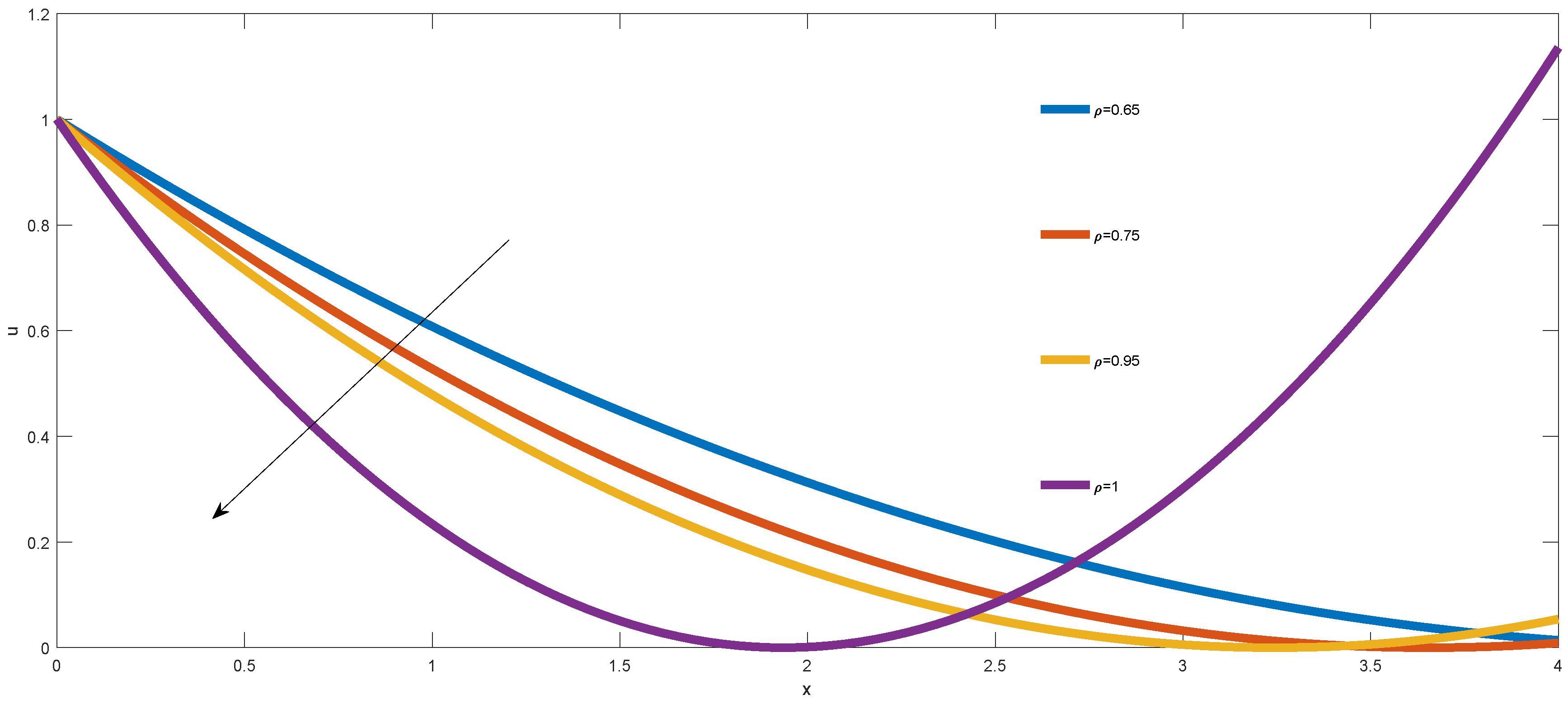
Let’s analyze some special cases. In Figure 1, we depict the behavior of the approximate solution when , and .
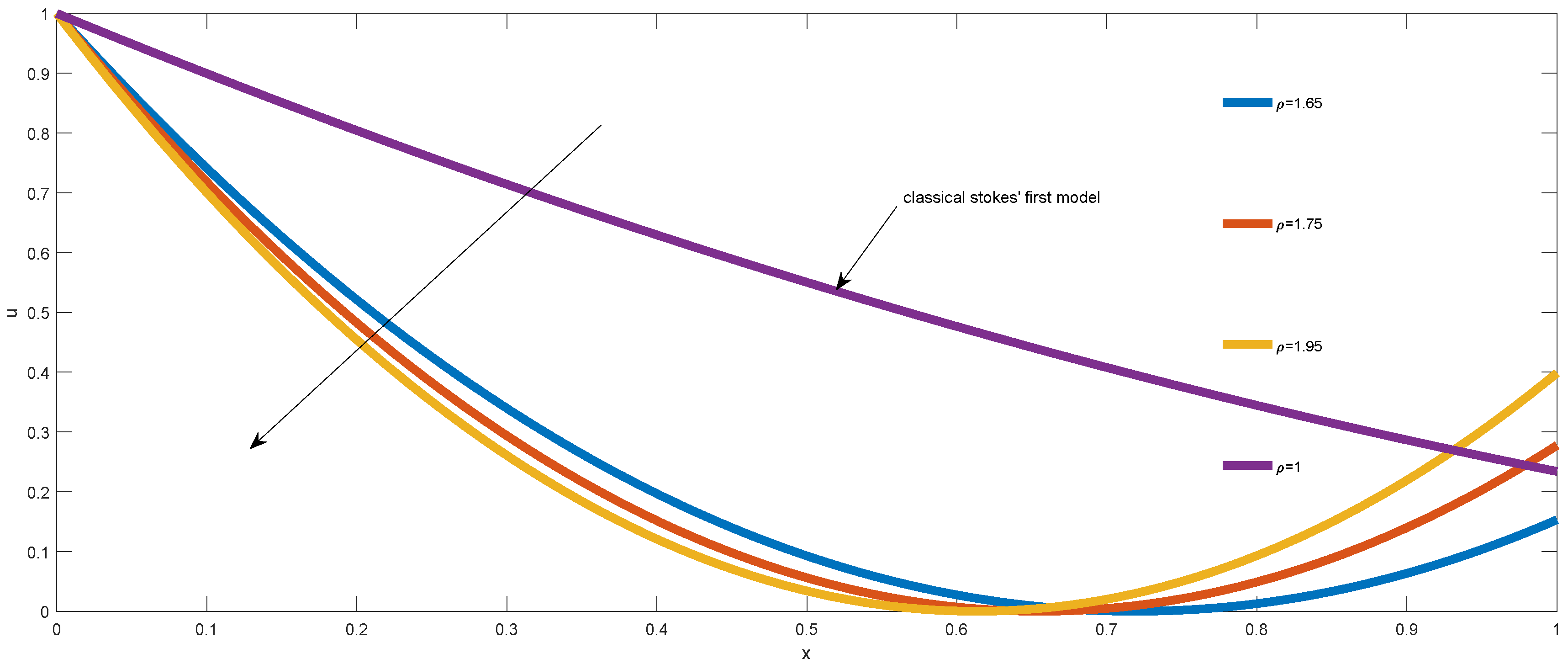
We notice all the curves decay in the space, by following the increase of the order . Observing the behavior of the classical Stokes’ first equation (), we note an acceleration impact in the diffusion process when the order . In Figure 2, we depict the behavior of the approximate solution when , and .
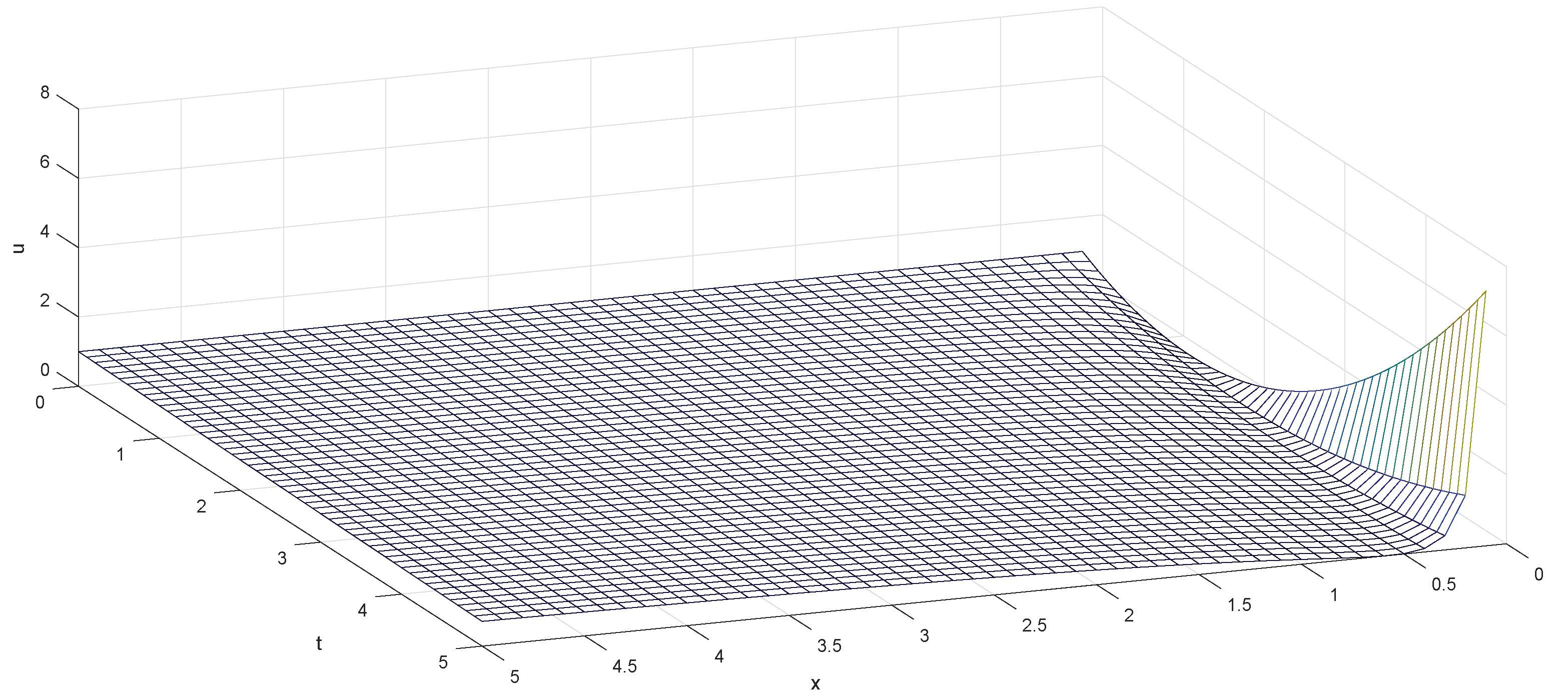
We notice all the curves decay in the space, by following the increase of the order . Observing the behavior of the classical Stokes’ first equation (), we note a retardation impact in the diffusion process when the order . In Figure 3, we depict the behavior of the approximate solution in the space and in the time with .
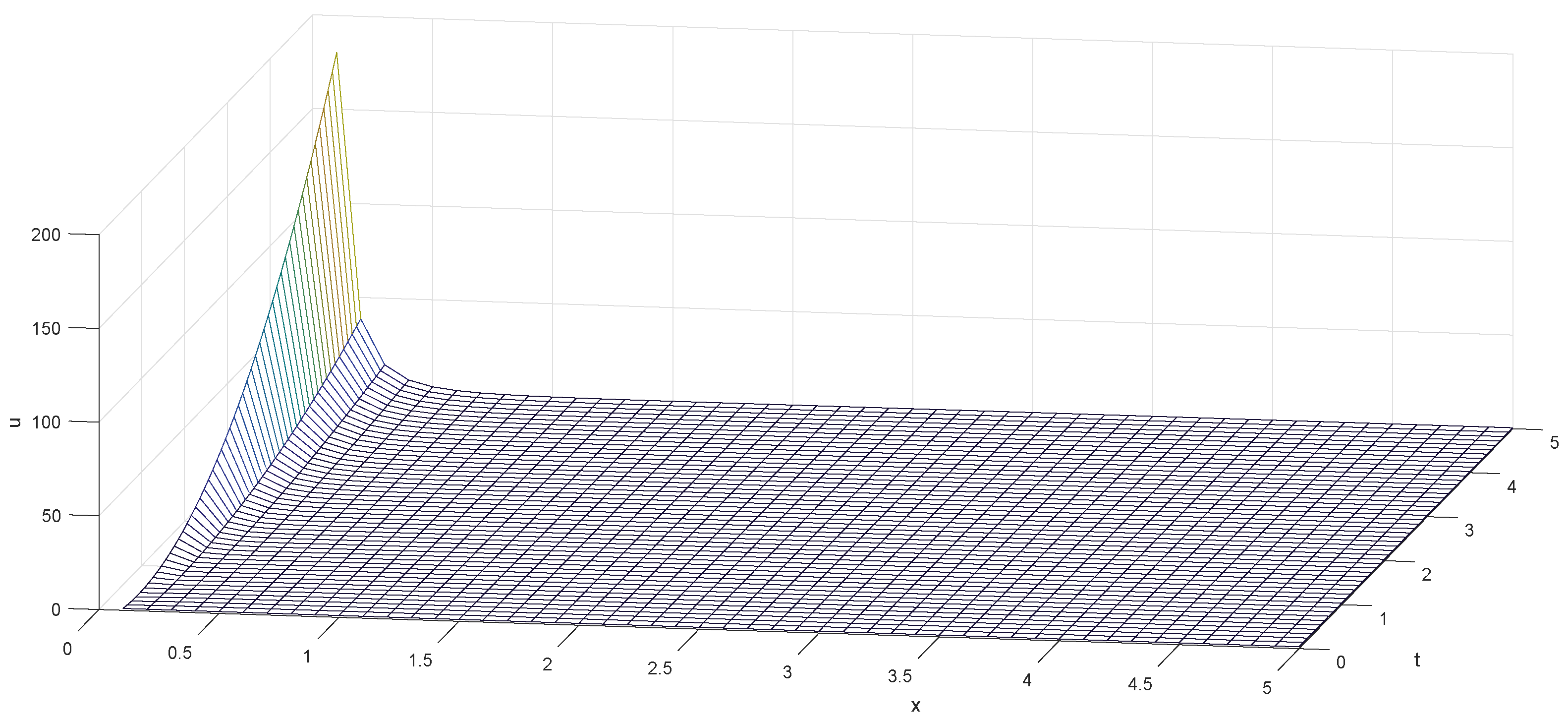
In Figure 4, we depict the behavior of the approximate solution in the space and the coordinate time with . It corresponds to Stokes’ first equation for Newtonian fluid.
7. Physical Discussion
In this section, we describe the physical meanings of our works briefly. The physical proposition of our works is to propose the flow profile of the Stokes’ first problem. Note that the similarity variable plays an important role in the determination of the flow profiles of the physical models. Our objective in this paper is to propose the flow of the Stokes’ first problem using the penetration depth, which is a physical method, by forgetting the mathematical aspect of the model (14). In other words, the model is a mathematical equation; it can be solved using many mathematical tools; here, we forget these tools and propose the flow profile using the physical concepts. The integral balance method is a good compromise to determine the flow profile by using the similarity variable. The HBIM and DIM propose the approximate value of the penetration depth. This penetration depth is used to give the similarity variable and to deduce the form of the flow profile. In our work, the similarity variable permit to classify the Stokes’ first problem in two classes: Stokes’ first problem for Newtonian fluid and the Stokes’ first problem for generalized second-grade fluid. Let us make and ; using the penetration depth Equation (23), the similarity variable is given by when , which represents the similarity variable of the Stokes’ first problem for a Newtonian fluid. Using the similarity variable, the exact flow profile for Newtonian fluid is given by
where denotes the Gaussian function. In general for a Newtonian fluid when the value of the exponent is arbitrary, the similarity variable is in the form . Let us have and . The similarity variable of the Stokes’ first problem coincides with the similarity variable for a heated second-grade fluid, for a long time of diffusion. With classical mathematical tools, the profile of the flow is difficult to be established, and the graphical representation of the solution is not trivial. Our method proposes the following approximate flow profile for Stokes’ first problem for a heated second-grade fluid
where we stipulate the exponent . The graphical representation of the flow is depicted in Figure 2. The above flow profile confirms Teipel works [29] on Stokes’ first equation. The similarity solution by series expansion is not possible [29]. Our observation is that, when the time of the diffusion process is very long, the similarity variable of the Stokes’ first problem can be obtained and is in the form when we use because the term converges to zero. A conclusion is that, when the time of the diffusion process is very long, we recover the similarity variable and the flow profile of the Newtonian fluid.
8. Optimization of the Residual Function
In this section, we give a brief exposition related to the Myers method of getting the exponent n of the assumed profile. Let us have the residual function of the Stokes’ first equation as
where is the approximate solution of the Stokes’ first equation. Let us define the Langford function defined by
Naturally by Myers, when the approximate solution is the exact solution or approach exact solution u, then the residual function should be zero or approach zero too. That is, Myers criterion of getting exponent n consists of finding an optimal n that minimizes the Langford function. A trivial consequence of the Myers criterion is that the residual function should attend its minimum for certain values of the exponent Thus, we can obtain the value of the exponent n at the boundary conditions ( and ). In other words, the Goodman condition should be satisfied:
We begin by recalling some calculations strategical for the Residual function:
We investigate the value of the . We first recall the Taylor expansion of the function . We have the following relation:
Thus, we have the following relationship:
The residual function of the Stokes’ first equation defined by Equation (14) is given by
At , in order to satisfy the Goodman conditions, the Residual function should be zero and then we have
At and , in order to satisfy the Goodman conditions, the Residual function should be zero and then we have
when Note that the exponent and found at the boundary conditions are not necessary for the optimal exponent that minimizes the Langford function. An alternative is finding n by minimizing the function
with the residual function defined by Equation (45). The result is not trivial. In this paper, we accept the optimal exponent in the previous section. The method used in Section 6 is more straightforward than the Myers criterion defined in this section. In conclusion, for the Stokes’ first equation, we assume that the approximate solution is quadratic. That is,
The penetration depth is obtained with HBIM method or the DIM method.
9. Conclusions
In this paper, we have discussed the approximate solution of the Stokes’ first equation described by the generalized fractional derivative. We have analyzed the impact of the order in the diffusion process. The order have in general a retardation or an acceleration effect in the diffusion process. Furthermore, the quadratic function is a good compromise to approach the exact solution of the Stokes’ first equation.
Funding
This research received no external funding.
Conflicts of Interest
The author declares no conflict of interest.
References
- Fetecau, C.; Fetecau, C. The Rayleigh–Stokes problem for heated second grade fluids. Int. J. -Non-Linear Mech. 2002, 37, 1011–1015. [Google Scholar] [CrossRef]
- Zierep, J. Similarity Laws and Modeling; Marcel Dekker Inc.: New York, NY, USA, 1971. [Google Scholar]
- Zierep, J. Das Rayleigh–Stokes Problem fur die Ecke. Acta Mech. 1979, 34, 161–165. [Google Scholar] [CrossRef]
- Bandelli, R.; Rajagopal, K.R. Start-up flows of second grade fluids in domains with one finite dimension. Int. J. Non-Linear Mech. 1995, 30, 817–839. [Google Scholar] [CrossRef]
- Owolabi, K.M.; Atangana, A. Robustness of fractional difference schemes via the Caputo subdiffusion-reaction equations. Chaos Solitons Fractals 2018, 111, 119–127. [Google Scholar] [CrossRef]
- Sene, N. Exponential form for Lyapunov function and stability analysis of the fractional differential equations. J. Math. Comput. Sci. 2018, 18, 388–397. [Google Scholar] [CrossRef] [Green Version]
- Masood Khan The Rayleigh–Stokes problem for an edge in a viscoelastic fluid with a fractional derivative model. Nonlinear Anal. Real World Appl. 2009, 10, 3190–3195. [CrossRef]
- Shen, F.; Tana, W.; Zhao, Y.; Masuokad, T. The Rayleigh–Stokes problem for a heated generalized second grade fluid with fractional derivative model. Nonlinear Anal. Realworld Appl. 2006, 7, 1072–1080. [Google Scholar] [CrossRef]
- Sene, N. Stokes’ first problem for heated flat plate with Atangana–Baleanu fractional derivative. Chaos Solitons Fractals 2018, 117, 68–75. [Google Scholar] [CrossRef]
- Chen, C.-M.; Liu, F.; Turner, I.; Anh, V. Numerical methods with fourth-order spatial accuracy for variable-order nonlinear Stokes’ first problem for a heated generalized second grade fluid. Comput. Math. Appl. 2011, 62, 971–986. [Google Scholar] [CrossRef]
- Srinivasan, S.; Rajagopal, K.R. Study of a variant of Stokes’ first and second problems for fluids with pressure dependent viscosities. Int. J. Eng. Sci. 2009, 47, 1357–1366. [Google Scholar] [CrossRef]
- Zhuang, P.-H.; Liu, Q.-X. Numerical method of Rayleigh–Stokes problem for heated generalized second grade fluid with fractional derivative. Appl. Math. Mech. 2009, 30, 1533–1546. [Google Scholar] [CrossRef]
- Yu, D.N.; He, J.H.; Garcıa, A.G. Homotopy perturbation method with an auxiliary parameter for nonlinear oscillators. J. Low Freq. Noise Vib. Act. Control 2018. [Google Scholar] [CrossRef]
- Anjum, N.; He, J.H. Laplace transform: Making the variational iteration method easier. Appl. Math. Lett. 2019, 92, 134–138. [Google Scholar] [CrossRef]
- Hristov, J. A transient flow of a non-Newtonian fluid modelled by a mixed time-space derivative: An improved integral-balance approach. Math. Methods Eng. 2019, 153–174. [Google Scholar] [CrossRef]
- Myers, T.G. Optimal exponent heat balance and refined integral methods applied to Stefan problems. Int. J. Heat Mass Transf. 2010, 53, 1119–1127. [Google Scholar] [CrossRef] [Green Version]
- Mitchell, S.L.; Myers, T.G. Improving the accuracy of heat balance integral methods applied to thermal problems with time dependent boundary conditions. Int. J. Heat Mass Transf. 2010, 53, 3540–3551. [Google Scholar] [CrossRef] [Green Version]
- Hristov, J. Fourth-order fractional diffusion model of thermal grooving: Integral approach to approximate closed form solution of the Mullins model. Math. Model. Nat. Phenom. 2018, 13, 6. [Google Scholar] [CrossRef]
- Fahd, J.; Abdeljawad, T. A modified Laplace transform for certain generalized fractional operators. Results Nonlinear Anal. 2018, 2, 88–98. [Google Scholar]
- Priyadharsini, S. Stability of fractional neutral and integrodifferential systems. J. Fract. Calc. Appl. 2016, 7, 87–102. [Google Scholar]
- Owolabi, K.M.; Hammouch, Z. Mathematical modeling and analysis of two-variable system with noninteger-order derivative. Chaos 2019, 1, 013145. [Google Scholar] [CrossRef]
- Sene, N. Analytical solutions of Hristov diffusion equations with non-singular fractional derivatives. Chaos 2019, 29, 023112. [Google Scholar] [CrossRef] [PubMed]
- Abdeljawad, T.; Mert, R.; Peterson, A. Sturm Liouville equations in the frame of fractional operators with exponential kernels and their discrete versions. Quest. Math. 2018, 1–19. [Google Scholar] [CrossRef]
- Makhlouf, A.B.; Nagy, A.M. Finite-time stability of linear Caputo–Katugampola fractional-order time delay systems. Asian J. Control. 2019, 21, 1–10. [Google Scholar] [CrossRef]
- He, J.H. Fractal calculus and its geometrical explanation. Results Phys. 2018, 10, 272–276. [Google Scholar] [CrossRef]
- Li, X.X.; Tian, D.; He, C.H.; He, J.H. A fractal modification of the surface coverage model for an electrochemical arsenic sensor. Electrochim. Acta 2019, 296, 491–493. [Google Scholar] [CrossRef]
- Wang, Q.L.; Shi, X.Y.; He, J.H.; Li, Z.B. Fractal calculus and its application to explanation of biomechanism of polar bear hairs. Fractals 2018, 26, 1850086. [Google Scholar] [CrossRef]
- Wang, Y.; Deng, Q. Fractal derivative model for tsunami travelling. Fractals 2019, 27, 1950017. [Google Scholar] [CrossRef]
- Teipel, I. The Impulsive Motion of a Flat Plate in a Viscoelastic Fluid. Acta Mechanica 1981, 39, 277–279. [Google Scholar] [CrossRef]
Figure 1.
Approximate solutions of Stokes’ first equation, , and .

Figure 2.
Approximate solutions of Stokes’ first equation, , and .

Figure 3.
Approximate solutions of Stokes’ first equation, , and .

Figure 4.
Approximate solutions of Stokes’ first equation, , and .

© 2019 by the author. Licensee MDPI, Basel, Switzerland. This article is an open access article distributed under the terms and conditions of the Creative Commons Attribution (CC BY) license (http://creativecommons.org/licenses/by/4.0/).
Share and Cite
MDPI and ACS Style
Sene, N. Integral Balance Methods for Stokes’ First Equation Described by the Left Generalized Fractional Derivative. Physics 2019, 1, 154-166. https://0-doi-org.brum.beds.ac.uk/10.3390/physics1010015
AMA Style
Sene N. Integral Balance Methods for Stokes’ First Equation Described by the Left Generalized Fractional Derivative. Physics. 2019; 1(1):154-166. https://0-doi-org.brum.beds.ac.uk/10.3390/physics1010015
Chicago/Turabian StyleSene, Ndolane. 2019. "Integral Balance Methods for Stokes’ First Equation Described by the Left Generalized Fractional Derivative" Physics 1, no. 1: 154-166. https://0-doi-org.brum.beds.ac.uk/10.3390/physics1010015