Extended SSH Model: Non-Local Couplings and Non-Monotonous Edge States

Abstract

We construct a generalized system by introducing an additional long-range hopping to the well-known Su-Schrieffer-Heeger (SSH) model. This system exhibits richer topological properties including non-trivial topological phases and associated localized edge states. We study the zero-energy edge states in detail and derive the edge-state wave functions using two different methods. Furthermore, we propose a possible setup using octupole moments optically excited on an array of dielectric particles for the realization of the system, and by adjusting the coupling strengths between neighboring particles we can control the hotspots (near-field enhancement) in such structures.

1. Introduction

One of the most important advances in recent decades in condensed matter physics has been the theoretical prediction [1,2] and experimental confirmation [2] of a new phase of matter called the ”topological insulator”. A topological insulator does not conduct current through the bulk, but its surface can conduct electricity without dissipation or back-scattering, even in the presence of large impurities. The first example of this was the integer quantum Hall effect, discovered in 1980. The discovery of topological insulator allows significant advances in spintronics [3,4,5], photonics devices [6] and quantum computing [7,8,9,10].

One of the simplest topological insulator models was proposed by Su, Schrieffer and Heeger in 1979 [11] which describes a particle hopping in 1D lattice with staggered hopping constants. It has been extensively studied both theoretically and experimentally. The starting point of this article is to extend the SSH model by adding additional hopping which preserves chiral symmetry. Although the extended SSH model with long-range hopping has already been investigated in a general sense [12], some important aspects of such generalization were overlooked. Here we study a specific model containing rich quantum phases protected by symmetries. Unlike SSH model, this system has two topologically non-trivial topological phases with winding number $\mathcal{W}=\pm 1$. This system supports localized zero-energy edge states associated with each non-trivial phase which exhibit non-monotonous spatial decay. We study the topological phases and associated edge states of this system in detail.

Another aspect of special interest in topological insulators are experimental implementations and demonstrations with artificial matter setups. Such demonstrations have been performed by engineering photonic crystals and metamaterials with synthetic magnetic fields and spin-orbit interactions [13,14,15,16], cold atoms and ions [17,18,19], plasmonic systems [20,21,22,23] and superconducting circuits [24,25,26,27,28,29]. These systems often employ periodic driving as a tool to engineer the effective Hamiltonian. We will also propose a possible realization of our model using nanoparticles based on polarization-dependent interactions between resonant modes of its structural elements.

This paper is organized as follows. In Section 2, the setup of our model is described, and its topological phases are characterized using the winding number. This system possesses chiral symmetry, which implies the existence of zero energy localized edge states when the system falls into topologically non-trivial phases, thus in Section 3 we derive the wave functions of these edge states using two different methods. In Section 4, we discuss a possible realization of this system using an array of nanoparticles. Finally, we present a summary and conclusion in Section 5.

2. SSH Model With Long-Range Hopping

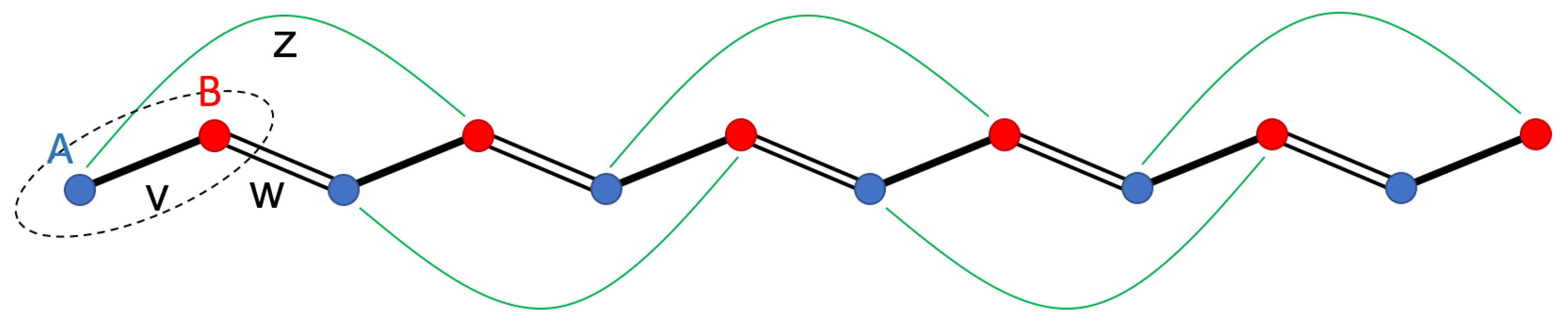
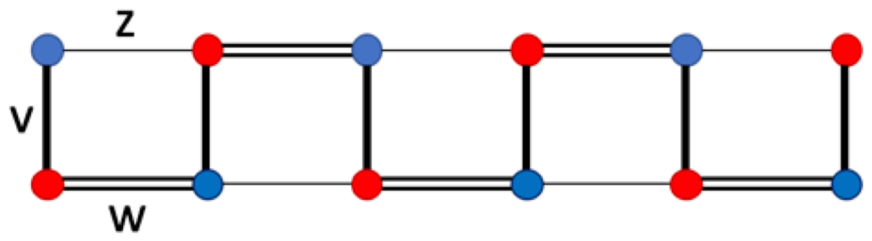
Similar to the standard SSH model, we consider a particle hopping in a 1D lattice (see Figure 1) which consists of N unit cells, each hosting two sites, A (blue) and B (red). The intra-cell and nearest-neighbor inter-cell hopping amplitudes are denoted by v and w, respectively. Furthermore, we introduce an additional hopping which connects sub-lattice A to sub-lattice B nonadjacent in two neighboring unit cells whose amplitude is denoted by z, as shown in Figure 1.

A single-particle Hamiltonian of this system can be expressed as follows

$$H=\sum _{j=1}^N(v{c}_{B,j}^{†}{c}_{A,j}+w{c}_{A,j+1}^{†}{c}_{B,j}+z{c}_{B,j+1}^{†}{c}_{A,j})+h.c.$$

(1)

where $c_{A,j}$ and $c_{B,j}$ stand for the annihilation operators of electron in sub-lattices A and B in the jth ($j\in \{1,2,\dots ,N\}$) unit cell, respectively. For simplicity, we set the hopping amplitudes to be real and non-negative. If the hopping amplitudes carried phases, the phase can always be gauged away by redefining the base states. The thermodynamical limit, $N\to \infty$, determines the most important properties of the model. To approach this thermodynamical limit, we can use the periodic boundary condition by simply closing the chain into a ring. With this boundary condition, the Hamiltonian can be transformed into momentum-space basis using

$$\begin{array}{c}\hfill c_{A,j}=\frac{1}{\sqrt{N}}\sum _k{e}^{ikj}{a}_k\\ \hfill c_{B,j}=\frac{1}{\sqrt{N}}\sum _k{e}^{ikj}{b}_k\end{array}$$

(2)

we can express Equation (1) as $H={\sum }_k{\psi }_k^{†}H\left(k\right){\psi }_k$ where ${\psi }_k$ is defined as ${\psi }_k={(a_k,b_k)}^T$ and $H\left(k\right)$ is the momentum-space Hamiltonian

$$H\left(k\right)=\left(\begin{array}{cc}0& \rho \left(k\right)\\ {\rho }^{*}\left(k\right)& 0\end{array}\right),\rho \left(k\right)=v+z{e}^{ik}+w{e}^{-ik}.$$

(3)

The eigenvalue of $H\left(k\right)$, $E\left(k\right)$, can be easily derived

$$\begin{array}{cc}\hfill E\left(k\right)=& \pm \left|\rho \right(k\left)\right|\hfill \\ \hfill =& \pm \sqrt{v^2+w^2+z^2-2wz+2v(w+z)\cos k+4wz{\cos }^{2}k}\hfill \end{array}$$

(4)

and provides with the dispersion relation of this system.

Introducing the vector of Pauli matrix $\sigma =({\sigma }_x,{\sigma }_y,{\sigma }_z)$, $H\left(k\right)$ can be expressed in a compact form

$$H\left(k\right)=\mathit{d}\left(k\right)·\sigma$$

(5)

with $\mathit{d}\left(k\right)=(d_x,d_y,d_z)=(v+z\cos k+w\cos k,w\sin k-z\sin k,0)$. Since vector $\mathit{d}\left(k\right)$ is lying in $d_x-d_y$ plane only, the chiral symmetry ${\sigma }_{z}H\left(k\right){\sigma }_z=-H\left(k\right)$ is preserved similar to the original SSH model. When k runs through the Brillouin zone from 0 to $2\pi$, the endpoint of $\mathit{d}\left(k\right)$ traces out a closed loop in $d_x-d_y$. For our system, this loop is an ellipsoid centered at point $(v,0)$, and the lengths of semi-major axis and semi-minor axis are $|w+z|$ and $|w-z|$, respectively. The $winding$ $number$ $\mathcal{W}$ is defined as the number of times this loop winds around the origin of the plane, expressed as

$$\mathcal{W}=\frac{1}{2\pi }{\int }_{-\pi }^{\pi }{\left(\tilde{\mathit{d}}\times \frac{d}{dk}\tilde{\mathit{d}}\left(k\right)\right)}_{z}dk.$$

(6)

where

$$\tilde{\mathit{d}}=\frac{\mathit{d}}{\left|\mathit{d}\right|}$$

(7)

is the projection of the closed loop onto a circle. This winding number can be written as an integral, using the complex logarithm function $\log \rho \left(k\right)=\log \left|\rho \right|+i\mathrm{Arg}\rho$. It can be proved that

$$\mathcal{W}=\frac{1}{2\pi i}{\int }_{-\pi }^{\pi }dk\frac{d}{dk}\log \rho \left(k\right).$$

(8)

From the mathematical point of view, the argument principle says that the derivative of $\log \rho \left(k\right)=\log \left|\rho \right|+i\mathrm{Arg}\rho$ where the total change in $\log \left|\rho \right|$ is zero for a closed contour counts the number of zeros/poles inside the contour with multiplicity weighted by the winding number. Simple computation yields the exact value of the winding number for systems with different parameters

$$\mathcal{W}=\left\{\begin{array}{cc}0,\hfill & |w+z|<v\hfill \\ 1,\hfill & |w+z|>vandw>z\hfill \\ -1,\hfill & |w+z|>vandw<z\hfill \end{array}\right.$$

(9)

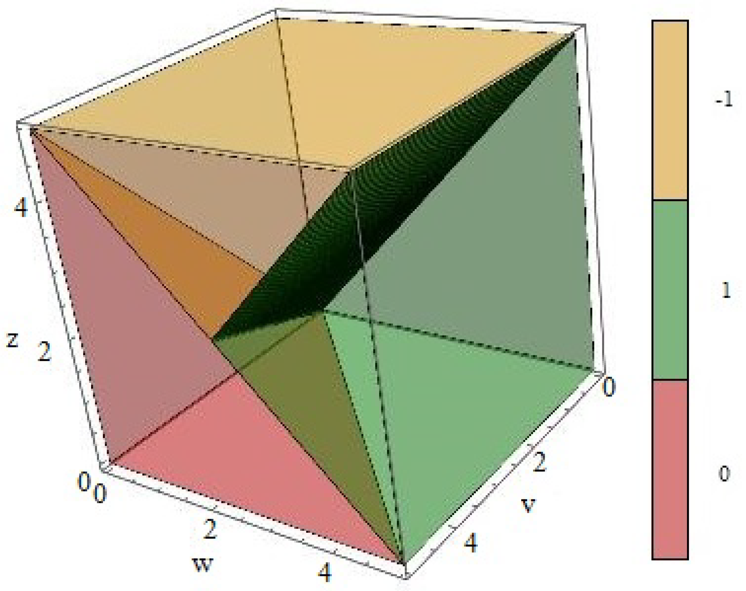
and the phase diagram is shown in Figure 2. The Zak phase [30], an analogue of the Berry phase for 1D systems, also carries important information about the system. Here, the Zak phase is related to the phase factor $\varphi \left(k\right)$ associated with $\rho \left(k\right)$ as $\rho \left(k\right)=\left|\rho \left(k\right)\right|e^{-i\varphi \left(k\right)}$ which is given by

$$\cot \varphi \left(k\right)=\frac{v}{(w-z)\sin k}+\frac{(w+z)\cot k}{w-z}.$$

(10)

And the Zak phase is defined as

$$\mathcal{Z}=\frac{1}{2}\oint dk\frac{d\varphi }{dk}=\frac{\Delta \varphi }{2}$$

(11)

where $\Delta \varphi$ is the total variation in phase $\varphi \left(k\right)$ when k varies across the full Brillouin zone.

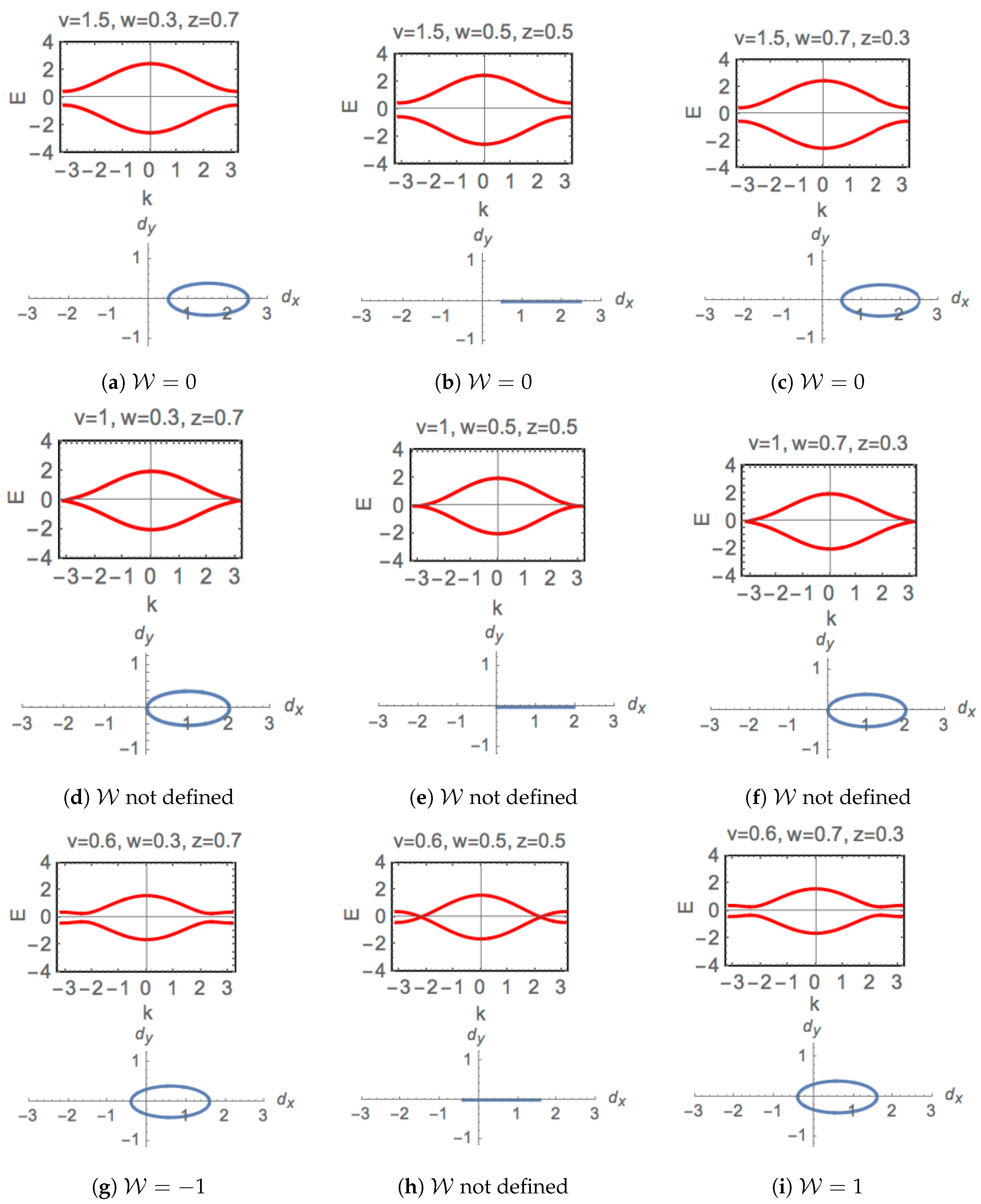
Topological phase transitions are always accompanied by closing of the energy band gaps. For our model, we show in Figure 3 the dispersion relation together with the corresponding trajectory of $\widehat{\mathit{d}}\left(k\right)$ for the system with nine different choices of parameters w, v and z. In the first, second, and third line, $v,w,z$ satisfy $v>w+z,v=w+z$ and $v<w+z$ respectively. In column 1 and 3, systems from top to bottom experience phase transitions from topologically trivial states to topologically non-trivial states, and there are closes of band gaps accompanying these transitions as shown by the cases in the second column. There is also a phase transition from $\mathcal{W}=-1$ to $\mathcal{W}=1$ as shown in the third row, and the close of the band gap associated with this transition manifests in Figure 3h in between.

In our model, only additional couplings (z) between 1 and 4 sites (3 and 6, 5 and 8, etc.) are considered. It seems natural to consider a simpler geometry with additional couplings between 1 and 3 sites (2 and 4, 3 and 5, etc.). In the case of this second neighbor coupling, assume that the coupling strength between ith and $(i+2)$th sites is $z_2$, then the momentum-space Hamiltonian reads

$$H_2\left(k\right)=\left(\begin{array}{cc}2z_2\cos k& v+w{e}^{-ik}\\ v+w{e}^{ik}& 2z_2\cos k\end{array}\right).$$

(12)

Chiral symmetry is absent in this Hamiltonian, thus such 1D lattices support no zero-energy edge state. In general, in order to preserve chiral symmetry, no coupling between ith and $(i+n)$th sites where n is an even number is allowed. However, odd couplings between site $2m-1$ and $(2m-1)+(2n+1)$ (i.e., subsite A in the mth unit cell and subsite B in the $(m+n)$th unit cell) where m enumerates the unit cells are allowed for all integer n if the chain is sufficiently long. The single-particle Hamiltonian of the generalized system with odd couplings can be expressed in the following form

$$H_o=H_{ssh}+\sum _{j=1}^N\sum _{n=1}{z}_n{c}_{B,j+n}^{†}{c}_{A,j}+h.c.$$

(13)

where $H_{ssh}$ is the Hamiltonian for the standard SSH model and $z_n$ denotes the coupling strength between site $2m-1$ and $(2m-1)+(2n+1)$ for every unit cell m. In this paper, we focus on the simplest system with the odd coupling z between site 1 and 4 (3 and 6, 5 and 8, etc.).

In systems with chiral symmetry, two states being chiral partners of each other must occur together. Bulk-edge correspondence (BEC), a theme in the theory of topological insulator, refers to a one-to-one correspondence between the topological invariant and the number of edge modes in a topologically non-trivial system. In a 1D chiral-symmetric lattice, the winding number is the topological invariant and it equals to the net number of edge modes on sub-lattice A at the left edge, $N_A-N_B$, where $N_A$ is the number of edge mode of sub-lattice A and $N_B$ is that of sub-lattice B, read from left [31]. When our system supports winding number $\mathcal{W}=1$ and $-1$ there is one edge mode, localized in sub-lattice A and B respectively seen from the left. Since each chiral pair is associated with opposite energies $\pm E$, and this single edge mode should satisfy it as well, thus E = 0. With zero energy, the wave functions of the edge states can be explicitly calculated without solving the eigen-problems. In the next section, we derive and characterize these edge states using two different methods, one incorporating the Zak phase and another one directly from the Hamiltonian.

3. Properties of the Edge States

3.1. Method 1: Edge-State Wave Functions Incorporating Zak Phase

As stated above, the edge states have zero energy and if forcing the bulk dispersion relation Equation (4) to be zero, i.e., $E\left(k_0\right)=0$, what information does this $k_0$ carry? In the rest of this section, it will be shown that the profile of the edge-state wave function can be easily obtained once $k_0$ is known. Noting that we are studying edge states which only occur in a topologically non-trivial system where the band gap of the dispersion relation is open, forcing the dispersion relation to be zero (a value inside the band gap) returns a complex number $k_0$:

$$k_0=-i\ln |\delta +\sqrt{{\delta }^2-1}|+Arg(\delta +\sqrt{{\delta }^2-1}),\delta =\frac{-v(w+z)}{4wz}+\frac{|w-z|}{4wz}\sqrt{v^2-4wz}$$

(14)

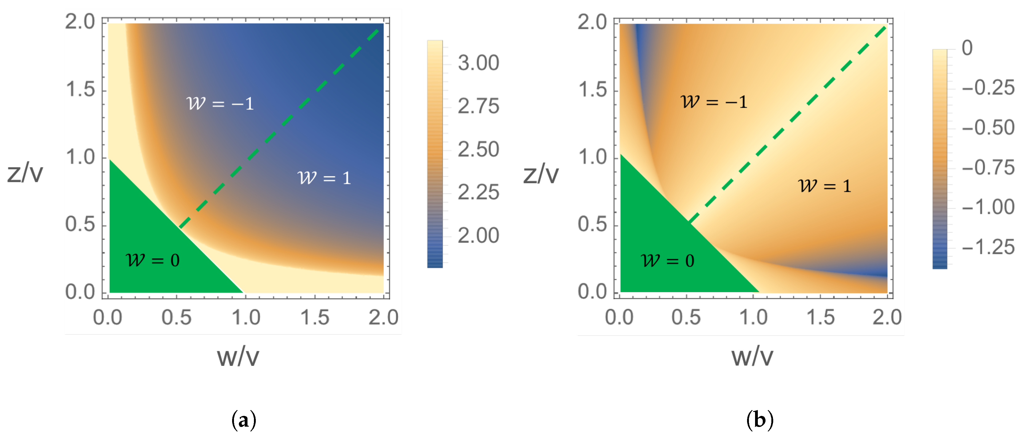
is a solution of $E\left(k_0\right)=0$. The real and imaginary part of $k_0$ have been plotted in Figure 4a,b, respectively, as functions of $w/v$ and $z/v$ in the topologically non-trivial regime, i.e., $z/v+w/v>1$. The real part of $k_0$ is strictly $\pi$ when $v^2-4wz\le 0$ and decreases with increasing w and z. We will show later that in the regime $v^2-4wz\le 0$, the coefficient amplitude for any edge state is strictly monotonic. The imaginary part equals to zero when $z=w$ which denotes the boundary of topological phase transition while decreases along $v^2-4wz=0$ with increasing w and z.

A general expression of wave functions on a dimerized 1D open lattice is given by [30]

$$|v_{\pm }\left(k\right)\rangle =\frac{i}{\sqrt{M}}\sum _m\left(\begin{array}{c}\sin [km-\varphi (k\left)\right]\\ \pm \sin \left(km\right)\end{array}\right).(|m,A\rangle ,|m,B\rangle )$$

(15)

where M is the total number of unit cells in the finite chain, $|m,A/B\rangle$ denotes the orbital $A/B$ in the mth cell and $\varphi \left(k\right)$ is the Zak phase. Using $\varphi \left(k\right)$ in Equation (10), the wave function Equation (15) above transforms into

$$|v_{\pm }\left(k\right)\rangle =\frac{i}{\sqrt{M}}\sum _m\left(\begin{array}{c}{\gamma }_m^A\\ {\gamma }_m^B\end{array}\right).(|m,A\rangle ,|m,B\rangle )$$

(16)

where

$$\left(\begin{array}{c}{\gamma }_m^A\\ {\gamma }_m^B\end{array}\right)=\left(\begin{array}{c}\left[w\sin \right(m-1)k+v\sin mk+z\sin (m+1\left)k\right]/\left|\rho \right(k\left)\right|\\ \pm \sin \left(km\right)\end{array}\right).$$

(17)

We only need to study the probability amplitude of one sub-lattice, since the other one can be obtained via the inversion symmetry, starting in the opposite direction. Here, ${\gamma }_m^A$ is the coefficient of interest. It can be expressed in the polar form as

$$\begin{array}{c}\hfill {\gamma }_m^A=\frac{1}{2i\left|\rho \right(k\left)\right|}\left(e^{imk}(w{e}^{-ik}+v+z{e}^{ik})-e^{-imk}(e^{ik}+v+z{e}^{-ik})\right)=\frac{\mathrm{Im}\left(e^{imk}\rho \left(k\right)\right)}{\left|\rho \right(k\left)\right|}.\end{array}$$

(18)

Writing $e^{imk}$ as $e^{imk}=e^{im\left(\mathrm{Re}\right(k)+i\mathrm{Im}(k\left)\right)}$ and $\rho \left(k\right)$ as $\rho \left(k\right)=\left|\rho \left(k\right)\right|e^{-i\varphi \left(k\right)}$, ${\gamma }_m^A$ can also be written as a composition of a sine wave and an exponential function:

$${\gamma }_m^A=e^{-\mathrm{Im}\left(k\right)m}\sin \left(\mathrm{Re}\left(k\right)m-\varphi \left(k\right)\right),$$

(19)

This form clearly demonstrates the roles of $\mathrm{Im}\left(k\right)$, $\mathrm{Re}\left(k\right)$ and $\varphi \left(k\right)$: $\mathrm{Im}\left(k\right)$ characterizes the exponential decay rate of the wave function along the chain, $\mathrm{Re}\left(k\right)$ describes the period of oscillation, and $\varphi \left(k\right)$ defines the initial phase of the sine wave. Plugging the wavenumber $k_0$, Equation (14), into Equation (19), one gets the wave function of the edge state. The form of Equation (19) also illustrates how the energy of a zero-energy wave incident the 1D lattice is dissipated during its travel; the coefficient of this wave decays exponentially with periodic fluctuations. Indeed, energy dissipation is the reason the edge state falls into the band gap of the energy spectrum; a wave with energy in the band gap is not propagating without loss, thus giving rise to a localized state showing a signature of dissipation. By carefully adjusting the parameters v, w, z of our system, we can design the profile of the localized edge state by choosing the exponential decay rate and period of oscillation.

There is a special case $v^2-4wz\le 0$, as shown in Figure 4a, where the real part of $k_0$ is strictly $\pi$, then $k_0$ can be expressed as $k_0=\pi +i\lambda$ where $\xi =1/\lambda$ is the localization length of the edge state [30]. And the wave function Equation (16) can be written in terms of $\lambda$, as

$$\begin{array}{cc}\hfill |v_{k,\pm }^e\rangle & =\frac{1}{\sqrt{M}}\sum _m{(-1)}^{m+1}\left(\begin{array}{c}{\chi }_m^A\\ {\chi }_m^B\end{array}\right).(|m,A\rangle ,|m,B\rangle ),\hfill \\ \hfill \left(\begin{array}{c}{\chi }_m^A\\ {\chi }_m^B\end{array}\right)& =\left(\begin{array}{c}[-w\sinh (m-1)\lambda +v\sinh m\lambda -z\sinh (m+1\left)\lambda \right]/\left|\rho \right(k\left)\right|\\ \pm \sinh \left(m\lambda \right)\end{array}\right).\hfill \end{array}$$

(20)

Since our finite open chain has M unit cells, the boundary condition that the wave function vanishes on subs-lattice A at the $(M+1)$th unit cell requires that

$$w\sinh M\lambda +z\sinh (M+2)\lambda -v\sinh (M+1)\lambda =0.$$

(21)

When the number of unit cell M is large, Equation (21) gives

$$\exp (-\lambda )\approx \frac{v}{2w}\pm \frac{\sqrt{v^2-4wz}}{2w}.$$

(22)

The ± sign implies the edge-state amplitude ${\chi }_A$ contains a combination of two hidden exponential functions with real exponents, and it can be proved that $|{\chi }_A|$ is strictly monotonic.

3.2. Method 2: Exact Solutions of Zero-Energy Edge States

In this section, we present a method to exactly calculate the discrete edge-state wavevector and the approximation of the wavevector to a continuous function in the thermodynamic limit, $N\to \infty$. We derive it without solving for the complex wavenumber $k_0$, which is cumbersome in a general case. In the thermodynamical limit $N\to \infty$, the wave function of the zero-energy edge state can be exactly calculated in the absence of translational invariance [31]. When the Hamiltonian (Equation (1)) acts on the zero-energy edge state $|\psi \rangle$, it gives

$$\widehat{H}|\psi \rangle =0.$$

(23)

The edge-state wave vector can be written as

$$|\psi \rangle =\sum _{m=1}^N(A_m{c}_{A,m}^{†}+B_m{c}_{B,m}^{†})|0\rangle$$

(24)

where m enumerates the unit cell indexes, $A_m$ and $B_m$ are the coefficients of the wave function on sub-lattice A and B of the mth unit cell respectively, $|0\rangle$ denotes the vacuum state and N is the number of unit cells. Equation (23) can be expanded into

$$\begin{array}{cc}\hfill \widehat{H}=& (\sum _{m=2}^{N-1}(v{A}_m+w{A}_{m+1}+z{A}_{m-1})c_{B,m}^{†}+(v{A}_1+w{A}_2)c_{B,1}^{†}+(v{A}_N+z{A}_{N-1})c_{B,N}^{†}\hfill \\ & +\sum _{m=2}^{N-1}(v{B}_m+w{B}_{m-1}+z{B}_{m+1})c_{A,m}^{†}+(v{B}_1+z{B}_2)c_{A,1}^{†}+(v{B}_N+w{B}_{N-1})c_{A,N}^{†})|0\rangle =0\hfill \end{array}$$

(25)

To make this equal to 0, the coefficient in front of every independent term must be equal to 0, which gives $2N$ linear equations:

$$v{A}_m+w{A}_{m+1}+z{A}_{m-1}=0$$

(26a)

$$v{B}_m+w{B}_{m-1}+z{B}_{m+1}=0$$

(26b)

($m=2,3,\dots ,N-1$) for the bulk, and

$$\begin{array}{cc}\hfill v{A}_1+w{A}_2=& 0\hfill \\ \hfill v{A}_N+z{A}_{N-1}=& 0\hfill \\ \hfill v{B}_1+z{B}_2=& 0\hfill \\ \hfill v{B}_N+w{B}_{N-1}=0\end{array}$$

(27)

at the boundary. Since $B_m=A_{N-m}$ due to inversion symmetry, it is sufficient to solve the amplitude for sub-lattice $A_m$, and then $B_m$ can be obtained accordingly by labeling the indexes of the unit cells from the opposite direction. Solving the recurrence formula Equation (26a) (see Appendix A), we get

$$A_m=\frac{A_1({\mathsf{\Lambda }}_1{\mathsf{\Lambda }}_2^{m-1}-{\mathsf{\Lambda }}_2{\mathsf{\Lambda }}_1^{m-1})+A_2({\mathsf{\Lambda }}_1^{m-1}-{\mathsf{\Lambda }}_2^{m-1})}{{\mathsf{\Lambda }}_1-{\mathsf{\Lambda }}_2}$$

(28)

for $m=3,4,\dots ,N-1$, where

$$\begin{array}{cc}\hfill {\mathsf{\Lambda }}_1=& \frac{-v+\sqrt[]{v^2-4wz}}{2w},{\mathsf{\Lambda }}_2=\frac{-v-\sqrt[]{v^2-4wz}}{2w}.\hfill \end{array}$$

(29)

The boundary condition Equation (27) allows us to simplify the above solution further into the following form:

$$A_m=\frac{{\mathsf{\Lambda }}_1^m-{\mathsf{\Lambda }}_2^m}{{\mathsf{\Lambda }}_1-{\mathsf{\Lambda }}_2}{A}_1$$

(30)

for $m=1,2,\dots ,N$.

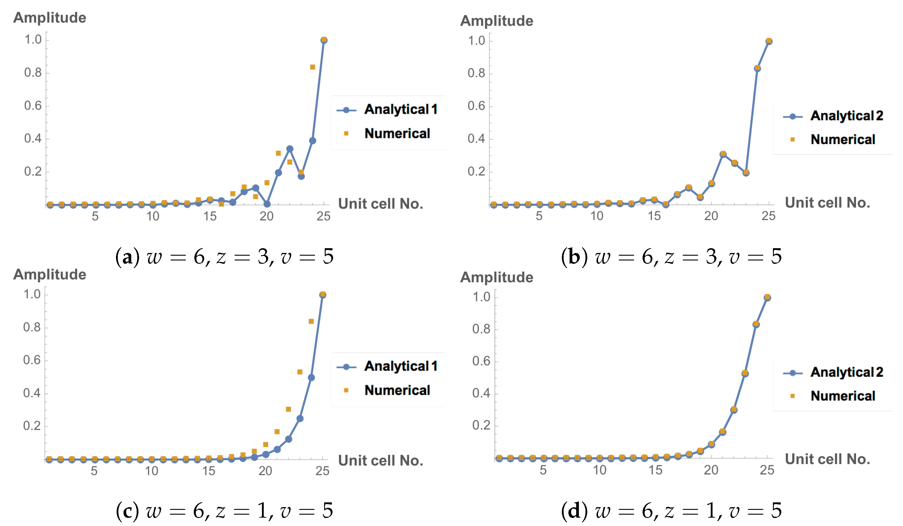
The edge-state wave function amplitudes for two different sets of parameters derived using method 1, discussed in last section, and method 2, comparing with the corresponding eigenvectors solved numerically from the Hamiltonian Equation (1), are plotted in Figure 5. For systems with $v^2-4wz<0$, as shown in the first row, the edge state amplitudes exhibit non-monotonicity and local maxima, but for systems with $v^2-4wz\ge 0$, such as the example in the second row, the edge states decay monotonously from the end. There are some discrepancies between the analytical solutions calculated using method 1 and the numerical results, which may be due to the assumption behind the general expression, Equation (15). When writing the wave function in that form, it is already assumed that the eigenvectors for open chains can be written as linear combinations of the bulk eigenfunctions [30], but in fact the bulk eigenfunctions may not be a set of complete bases to construct the edge states of open chains.

The thermodynamical limit, $N\to \infty$, determines the most important properties of the system. In the thermodynamic limit, the discrete wavevector of the edge state can be approximated by a continuous and smooth function evaluated at the particle sites [30,31]. With a smooth function rather than a sequence of seemingly disordered discrete points such as those shown in Figure 5a,b, we can see the behavior of waves propagating on the lattice and the energy dissipation of these waves more clearly. In the rest of this section we will find such approximations for our model and the standard SSH model and propose a possible generalization of this method to SSH systems with additional odd couplings. The starting point of this approximation is from approximating the recurrence equation that describes the edge-state wave functions, e.g., Equation (26a) to a differential equation of the same order by taking the reverse process of the well-known Euler method by replacing $A_n$ by A, the difference ratio $(A_{n+1}-A_n)/ϵ$ by $dA/dx$, the difference ratio of difference ratios,

$$\frac{1}{ϵ}(\frac{A_{n+2}-A_{n+1}}{ϵ}-\frac{A_{n+1}-A_n}{ϵ})=\frac{A_{n+2}-2A_{n+1}+A_n}{{ϵ}^2},$$

(31)

by $d^{2}A/d{x}^2$ …, where $ϵ$ is the distance between the A-subsites in two neighboring unit cells and $A\left(x\right)$ is the approximated continuous function. There is only one restriction, $A_m=A\left(mϵ\right)$, meaning that the continuous coefficient $A\left(x\right)$ evaluated at the mth particle must equal to the coefficient of this particle calculated using the discrete method.

Consider the standard SSH model first. The additional z-coupling vanishes, then the recurrence equation, Equation (26a), reduces to

$$v{A}_m+w{A}_{m+1}=0.$$

(32)

This can be easily solved by

$$A_m={(-\frac{v}{w})}^{m-1}{A}_1.$$

(33)

Due to the one-one correspondence between difference equations and differential equations of the same order, Equation (33) can be approximated by the solution of a first order differential equation

$$a\frac{dA}{dx}+bA=0.$$

(34)

where a and b are some constants. The general solution of this differential equation reads

$$A\left(t\right)=A\left(0\right)e^{-\frac{b}{a}x}.$$

(35)

This can be compared to the discrete solution, Equation (33), by writing

$${(-\frac{v}{w})}^n=\exp (n\ln (-\frac{v}{w}))=\exp \left(\kappa n\right)$$

(36)

where $\kappa =\ln (-v/w)$, then Equation (33) can be written as

$$A_m=A_1{e}^{\kappa (m-1)}.$$

(37)

This can be fitted to the exponential function $A\left(x\right)$, Equation (35), such that $A_m=A\left(mϵ\right)$, provided

$$\begin{array}{c}\frac{b}{a}=-\frac{\kappa }{ϵ}\hfill \\ A\left(0\right)=A_1{e}^{\frac{bϵ}{a}}.\hfill \end{array}$$

(38)

The wave function amplitudes read

$$|A_m|=|A_1|e^{-(m-1)/\chi }$$

(39)

where $\chi =1/(\ln w-\ln v)$ is the localization length, which is consistent with that calculated in ref. [31].

In terms of our model (1 additional odd couplings), the recurrence formula, Equation (26a), can be approximated by a second-order differential equation

$$\frac{d^{2}A}{d{x}^2}+2\alpha \frac{dA}{dx}+\beta A=0,$$

(40)

where $\alpha$ and $\beta$ are constant. The general solution of Equation (40) can be expressed by the roots ${\lambda }_1$, ${\lambda }_2$ of the characteristic equation ${\lambda }^2+2\alpha \lambda +{\beta }^2=0$ and the initial conditions $A\left(0\right)$ and $\dot{A}\left(0\right)=\frac{dA}{dx}\left(0\right)$:

$$A\left(x\right)=\frac{\dot{A}\left(0\right)-{\lambda }_{2}A\left(0\right)}{{\lambda }_1-{\lambda }_2}{e}^{{\lambda }_{1}x}+\frac{\dot{A}\left(0\right)-{\lambda }_{1}A\left(0\right)}{{\lambda }_2-{\lambda }_1}{e}^{{\lambda }_{2}x}.$$

(41)

To satisfy the restriction $A\left(mϵ\right)=A_m$, the crucial point is to set

$${\mathsf{\Lambda }}_k^n=\exp \left(n\ln {\mathsf{\Lambda }}_k\right)=\exp \left(nϵ{\lambda }_k\right)$$

(42)

where $k=1,2$, meaning that

$${\lambda }_k:={ϵ}^{-1}\ln {\mathsf{\Lambda }}_k$$

(43)

Then $A_n$ in Equation (30) can be rewritten in the form

$$A_n=\frac{A_1}{e^{ϵ{\lambda }_1}-e^{ϵ{\lambda }_2}}(e^{{\lambda }_{1}nϵ}-e^{{\lambda }_{2}nϵ})=A\left(nϵ\right)$$

(44)

as the continuous coefficient Equation (41) evaluated at discretized points $ϵm$, provided the initial conditions

$$\begin{array}{c}\hfill A\left(0\right)=\frac{2A_1}{e^{ϵ{\lambda }_1}-e^{ϵ{\lambda }_2}}\\ \hfill \dot{A}\left(0\right)=\frac{1}{2}({\lambda }_1+{\lambda }_2)A\left(0\right).\end{array}$$

(45)

The continuous function Equation (40) approximates the discrete equation Equation (30) such that

$$\frac{v}{w}=-2e^{-ϵ\alpha }\cos (ϵ\sqrt{{\beta }^2-{\alpha }^2}),\frac{z}{w}=e^{-2ϵ\alpha }.$$

(46)

Therefore, the zero-energy edge wave function for our system can be approximated by a combination of two exponential functions. If ${\lambda }_1$ and ${\lambda }_2$ in Equation (41) are complex numbers, $A\left(x\right)$ can be rewritten in the form of an exponential function with real exponent multiplied by a sin/cos wave, which is consistent with the form calculated using method 1.

Consider the general Hamiltonian with M additional odd couplings, Equation (13)

$$H_o=H_{ssh}+\sum _{j=1}^N\sum _{i=1}^M{z}_i{c}_{B,j+i}^{†}{c}_{A,j}+h.c.$$

(47)

which respects Chiral symmetry. In this case, subsite A in each unit cell j is coupled to subsite B in unit cell $j+1,j+2,\dots ,j+M$. The recurrence equation that gives the edge-state wavevector for this Hamiltonian, obtained from $H_0|\psi \rangle =0$ thus is

$$\sum _{i=1}^M{z}_{M-i+1}{A}_i+v{A}_{M+1}+w{A}_{M+2}=0$$

(48)

whose solution $A_n$ can be approximated by the continuous solution of a $(M+1)$th order differential equation, $A\left(x\right)$, i.e., $A_n=A\left(ϵn\right)={\sum }_{i=1}^{M+1}{C}_i\exp \left(ϵ{\lambda }_{i}n\right)$ where ${\lambda }_{1,\dots ,M+1}$ and $C_{1,\dots ,M+1}$ are constants to be determined. However, connections between the parameters ${\lambda }_{1,\dots ,M+1}$, $C_{1,\dots ,M+1}$ and the coupling strengths $z_{1,\dots ,M+1},v,w$ must be carefully calculated by solving the recurrence equation Equation (48) using generating functions or other methods, which is out of the scope of this paper.

4. Possible Physical Realization Using Array of Nanoparticles

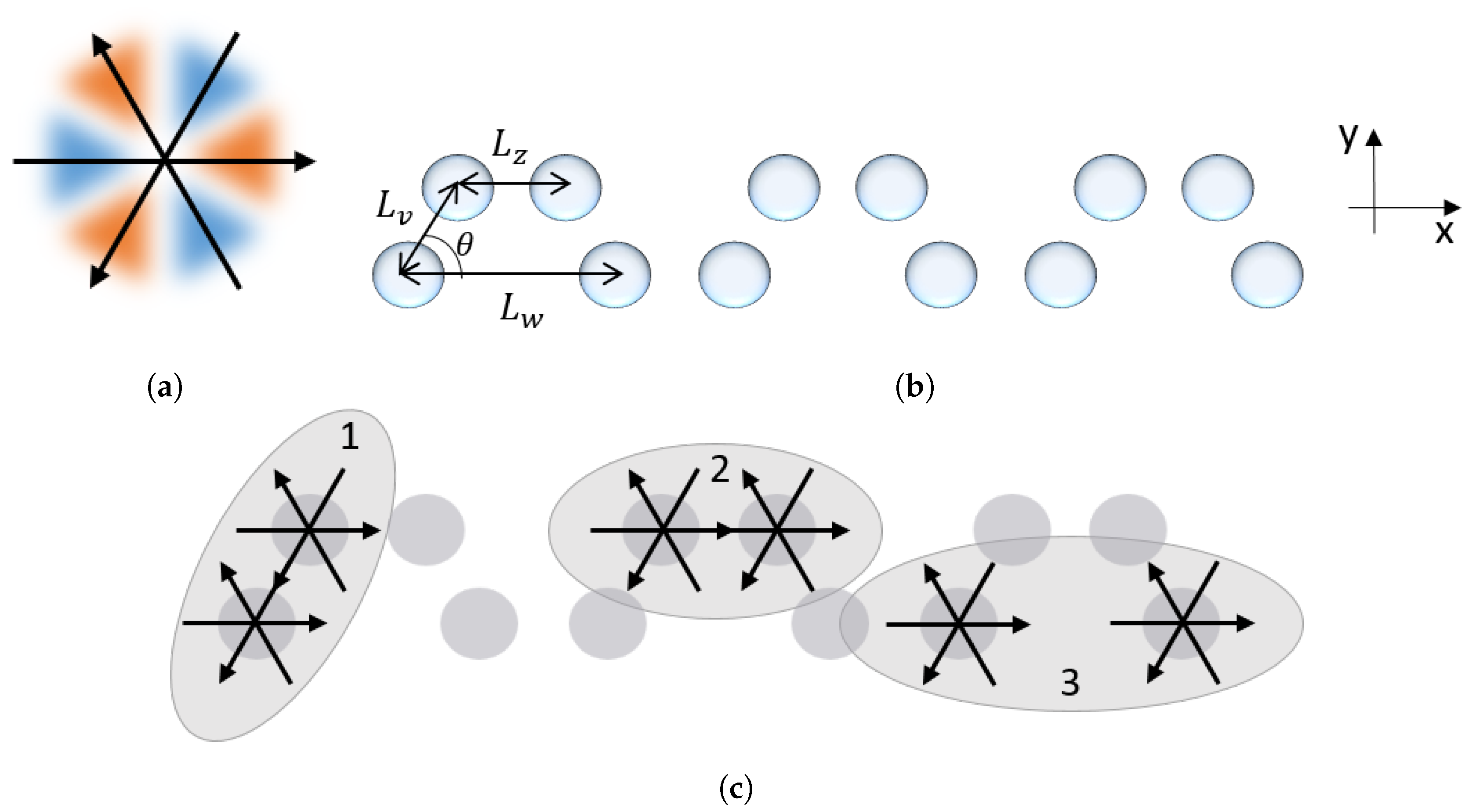
Here we propose a possible realization of our model using optically resonant nanoparticles which was successfully used in the past [15,20,32]. The geometry of our model in Figure 1 can be rearranged into a ladder system as shown in Figure 6. With this setup, the topological properties of our model can be demonstrated in an array of resonant nanoparticles shown in Figure 7b where an octupole moment is excited (as shown in Figure 7a) in each particle at the normal light incidence upon plane $x-y$.

Three major types of interaction between neighboring octupole moments in this setup are depicted in Figure 7c where the interaction strengths for type 1, 2, 3 correspond to the hopping amplitudes v, z and w, and they are controlled by angle $\theta$ and distance $L_v$, $L_z$, $L_w$ respectively (see Figure 7b).

Efficient heat generation in localized spots using plasmonic nanoparticles and optical excitation is an interesting field that has been extensively researched due to its wide potential applications in bio-related research [33], thermal actuation of biosystem [34], efficient light-to-heat conversion [35] and local temperature sensing in nanoscale systems [36]. The advantage of our system is the ability of controlling the locations of local maxima of the probability amplitude of the edge states by carefully adjusting the coupling strength w, v, z governing the periodicity, decay rate and initial phase of the amplitude profiles, which provides a potential method of fabricating the locations of hotspots in the array. As the edge states are protected by topology and symmetry, the hotspots generated by our system are robust to small perturbations.

5. Conclusions

By introducing extra hopping between two neighboring unit cells, a novel system with rich topological properties emerge. This system possesses more topological phases than the SSH model does, and the zero-energy edge state is a combination of exponential functions and sometimes can be written as an exponential decay modulated by cosine/sine waves. By adjusting the system parameters, we can control the period, initial phase and decay rate of the edge-state wavevector, which offers a way to fabricate the locations of hotspots (local maxima in the wave function), once the topolgical properties of our system can be realized on dielectric or plasmonic arrays. Since the edge states are protected by symmetry and topology, the hotspots in these states work as efficient and localized heat generation sources. We believe our model has potential applications in a wide range of fields such as biomedical systems, temperature sensing, near-field imaging, and hot-electron dynamics.

References

- Kane, C.L.; Mele, E.J. Z2 Topological Order and the Quantum Spin Hall Effect. Phys. Rev. Lett. 2005, 95, 146802. [Google Scholar] [CrossRef] [PubMed]
- Bernevig, B.A.; Hughes, T.L.; Zhang, S.C. Quantum Spin Hall Effect and Topological Phase Transition in HgTe Quantum Wells. Science 2006, 314, 1757–1761. [Google Scholar] [CrossRef] [PubMed] [Green Version]
- Pesin, D.; MacDonald, A.H. Spintronics and pseudospintronics in graphene and topological insulators. Nat. Mater. 2012, 11, 409–416. [Google Scholar] [CrossRef] [PubMed] [Green Version]
- Vobornik, I.; Manju, U.; Fujii, J.; Borgatti, F.; Torelli, P.; Krizmancic, D.; Hor, Y.S.; Cava, R.J.; Panaccione, G. Magnetic Proximity Effect as a Pathway to Spintronic Applications of Topological Insulators. Nano Lett. 2011, 11, 4079–4082. [Google Scholar] [CrossRef] [PubMed]
- Sinova, J.; Zutic, I. New moves of the spintronics tango. Nat. Mater. 2012, 11, 368–371. [Google Scholar] [CrossRef] [PubMed]
- Liu, M.; Cai, Z.R.; Hu, S.; Luo, A.P.; Zhao, C.J.; Zhang, H.; Xu, W.C.; Luo, Z.C. Dissipative rogue waves induced by long-range chaotic multi-pulse interactions in a fiber laser with a topological insulator-deposited microfiber photonic device. Opt. Lett. 2015, 40, 4767–4770. [Google Scholar] [CrossRef] [PubMed]
- Alicea, J.; Oreg, Y.; Refael, G.; von Oppen, F.; Fisher, M.P.A. Non-Abelian statistics and topological quantum information processing in 1D wire networks. Nat. Phys. 2011, 7, 412–417. [Google Scholar] [CrossRef] [Green Version]
- Hassler, F.; Akhmerov, A.R.; Hou, C.Y.; Beenakker, C.W.J. Anyonic interferometry without anyons: How a flux qubit can read out a topological qubit. New J. Phys. 2010, 12, 125002. [Google Scholar] [CrossRef]
- Ferreira, G.J.; Loss, D. Magnetically Defined Qubits on 3D Topological Insulators. Phys. Rev. Lett. 2013, 111, 106802. [Google Scholar] [CrossRef] [PubMed]
- Leijnse, M.; Flensberg, K. Quantum Information Transfer between Topological and Spin Qubit Systems. Phys. Rev. Lett. 2011, 107, 210502. [Google Scholar] [CrossRef] [PubMed]
- Su, W.P.; Schrieffer, J.R.; Heeger, A.J. Solitons in Polyacetylene. Phys. Rev. Lett. 1979, 42, 1698–1701. [Google Scholar] [CrossRef]
- Pérez-González, B.; Bello, M.; Gómez-León, Á.; Platero, G. SSH model with long-range hoppings: Topology, driving and disorder. arXiv, 2018; arXiv:1802.03973. [Google Scholar]
- Lu, L.; Joannopoulos, J.D.; Soljacic, M. Topological states in photonic systems. Nat. Phys. 2016, 12, 626–629. [Google Scholar] [CrossRef] [Green Version]
- Lu, L.; Joannopoulos, J.D.; Soljacic, M. Topological photonics. Nat. Photonics 2014, 8, 821–829. [Google Scholar] [CrossRef] [Green Version]
- Slobozhanyuk, A.P.; Poddubny, A.N.; Miroshnichenko, A.E.; Belov, P.A.; Kivshar, Y.S. Subwavelength Topological Edge States in Optically Resonant Dielectric Structures. Phys. Rev. Lett. 2015, 114, 123901. [Google Scholar] [CrossRef] [PubMed]
- Noh, C.; Rodriguez-Lara, B.M.; Angelakis, D.G. Proposal for realization of the Majorana equation in a tabletop experiment. Phys. Rev. A 2013, 87, 040102. [Google Scholar] [CrossRef]
- Duca, L.; Li, T.; Reitter, M.; Bloch, I.; Schleier-Smith, M.; Schneider, U. An Aharonov-Bohm interferometer for determining Bloch band topology. Science 2015, 347, 288–292. [Google Scholar] [CrossRef] [PubMed]
- Jotzu, G.; Messer, M.; Desbuquois, R.; Lebrat, M.; Uehlinger, T.; Greif, D.; Esslinger, T. Experimental realization of the topological Haldane model with ultracold fermions. Nature 2014, 515, 237–240. [Google Scholar] [CrossRef] [PubMed] [Green Version]
- Goldman, N.; Juzeliunas, G.; Ohberg, P.; Spielman, I.B. Light-induced gauge fields for ultracold atoms. Rep. Prog. Phys. 2014, 77, 126401. [Google Scholar] [CrossRef] [PubMed] [Green Version]
- Poddubny, A.; Miroshnichenko, A.; Slobozhanyuk, A.; Kivshar, Y. Topological Majorana States in Zigzag Chains of Plasmonic Nanoparticles. ACS Photonics 2014, 1, 101–105. [Google Scholar] [CrossRef]
- Ling, C.W.; Xiao, M.; Chan, C.T.; Yu, S.F.; Fung, K.H. Topological edge plasmon modes between diatomic chains of plasmonic nanoparticles. Opt. Express 2015, 23, 2021–2031. [Google Scholar] [CrossRef] [PubMed] [Green Version]
- Liu, C.X.; Dutt, M.V.G.; Pekker, D. Robust manipulation of light using topologically protected plasmonic modes. Opt. Express 2018, 26, 2857–2872. [Google Scholar] [CrossRef] [PubMed] [Green Version]
- Downing, C.A.; Weick, G. Topological collective plasmons in bipartite chains of metallic nanoparticles. Phys. Rev. B 2017, 95, 125426. [Google Scholar] [CrossRef]
- Koch, J.; Houck, A.A.; Le Hur, K.; Girvin, S.M. Time-reversal-symmetry breaking in circuit-QED-based photon lattices. Phys. Rev. A 2010, 82, 043811. [Google Scholar] [CrossRef] [Green Version]
- Nunnenkamp, A.; Koch, J.; Girvin, S.M. Synthetic gauge fields and homodyne transmission in Jaynes-Cummings lattices. New J. Phys. 2011, 13, 095008. [Google Scholar] [CrossRef]
- Mei, F.; You, J.B.; Nie, W.; Fazio, R.; Zhu, S.L.; Kwek, L.C. Simulation and detection of photonic Chern insulators in a one-dimensional circuit-QED lattice. Phys. Rev. A 2015, 92, 041805. [Google Scholar] [CrossRef]
- Mei, F.; Xue, Z.Y.; Zhang, D.W.; Tian, L.; Lee, C.H.; Zhu, S.L. Witnessing topological Weyl semimetal phase in a minimal circuit-QED lattice. Quantum Sci. Technol. 2016, 1, 015006. [Google Scholar] [CrossRef] [Green Version]
- Yang, Z.H.; Wang, Y.P.; Xue, Z.Y.; Yang, W.L.; Hu, Y.; Gao, J.H.; Wu, Y. Circuit quantum electrodynamics simulator of flat band physics in a Lieb lattice. Phys. Rev. A 2016, 93, 062319. [Google Scholar] [CrossRef]
- Tangpanitanon, J.; Bastidas, V.M.; Al-Assam, S.; Roushan, P.; Jaksch, D.; Angelakis, D.G. Topological Pumping of Photons in Nonlinear Resonator Arrays. Phys. Rev. Lett. 2016, 117, 213603. [Google Scholar] [CrossRef] [PubMed]
- Delplace, P.; Ullmo, D.; Montambaux, G. Zak phase and the existence of edge states in graphene. Phys. Rev. B 2011, 84, 195452. [Google Scholar] [CrossRef]
- Asbóth, J.K.; Oroszlány, L.; Pályi, A. A Short Course on Topological Insulators: Band-structure topology and edge states in one and two dimensions. arXiv, 2015; arXiv:1509.02295. [Google Scholar]
- Sinev, I.S.; Mukhin, I.S.; Slobozhanyuk, A.P.; Poddubny, A.N.; Miroshnichenko, A.E.; Samusev, A.K.; Kivshar, Y.S. Mapping plasmonic topological states at the nanoscale. Nanoscale 2015, 7, 11904–11908. [Google Scholar] [CrossRef] [PubMed]
- Cognet, L.; Tardin, C.; Boyer, D.; Choquet, D.; Tamarat, P.; Lounis, B. Single metallic nanoparticle imaging for protein detection in cells. Proc. Natl. Acad. Sci. USA 2003, 100, 11350–11355. [Google Scholar] [CrossRef] [PubMed] [Green Version]
- Assanov, G.S.; Zhanabaev, Z.Z.; Govorov, A.O.; Neiman, A.B. Modelling of photo-thermal control of biological cellular oscillators. Eur. Phys. J. Spec. Top. 2013, 222, 2697–2704. [Google Scholar] [CrossRef] [PubMed] [Green Version]
- Richardson, H.H.; Carlson, M.T.; Tandler, P.J.; Hernandez, P.; Govorov, A.O. Experimental and Theoretical Studies of Light-to-Heat Conversion and Collective Heating Effects in Metal Nanoparticle Solutions. Nano Lett. 2009, 9, 1139–1146. [Google Scholar] [CrossRef] [PubMed] [Green Version]
- Capobianco, J.A.; Vetrone, F.; D’Alesio, T.; Tessari, G.; Speghini, A.; Bettinelli, M. Optical spectroscopy of nanocrystalline cubic Y2O3: Er3+ obtained by combustion synthesis. Phys. Chem. Chem. Phys. 2000, 2, 3203–3207. [Google Scholar] [CrossRef]
Figure 1.
Schematic of the extended SSH model.
Figure 2.
Phase diagram indicating the topological phases characterized by the winding number for systems with different hopping parameters. Yellow, red, and green represent , 0 and 1 respectively.
Figure 3.
Dispersion relations, Equation (4) together with the corresponding vector , Equation (5), on plane as the wavenumber k is swept across the Brillouin zone, for nine different settings of hopping amplitudes: (a) , , ; (b) , , ; (c) , , ; (d) , , ; (e) , , ; (f) , , ; (g) , , ; (h) , , ; (i) , , .
Figure 4.
(a) Real part and (b) imaginary part of the complex number , plotted as functions of and in the topologically non-trivial regime, i.e., . The green area in each plot corresponds to topologically trivial region with winding number . The regions with and 1 are also labeled in the figures. Note that, as shown in (b), phase transition occurs at where dose not decay, i.e., the localized edge states vanish.
Figure 5.
Coefficient amplitudes for two different sets of parameters, , , in the first row and , , in the second row, calculated on a finite chain with 25 unit cells using method 1 and method 2: (a) , , using method 1; (b) , , using method 2; (c) , , using method 1; (d) , , using method 2; The discrete dots represent the edge-state amplitudes numerically given by the eigenvector of the Hamiltonian Equation (1).
Figure 6.
Rearrangement of the geometry shown in Figure 1 as a ladder system.
Figure 7.
(a) A cross-section of the octupole moment excited on each particle; (b) Arrangement of the nanoparticle array; (c) Three major interactions between neighboring particles, 1, 2 and 3, which mimic the hopping amplitudes, v, z and w respectively. The strengths of these interactions can be controlled by varying the distances, , , , and angle .
© 2018 by the authors. Licensee MDPI, Basel, Switzerland. This article is an open access article distributed under the terms and conditions of the Creative Commons Attribution (CC BY) license (http://creativecommons.org/licenses/by/4.0/).
Share and Cite
MDPI and ACS Style
Li, C.; Miroshnichenko, A.E. Extended SSH Model: Non-Local Couplings and Non-Monotonous Edge States. Physics 2019, 1, 2-16. https://0-doi-org.brum.beds.ac.uk/10.3390/physics1010002
AMA Style
Li C, Miroshnichenko AE. Extended SSH Model: Non-Local Couplings and Non-Monotonous Edge States. Physics. 2019; 1(1):2-16. https://0-doi-org.brum.beds.ac.uk/10.3390/physics1010002
Chicago/Turabian StyleLi, Chao, and Andrey E. Miroshnichenko. 2019. "Extended SSH Model: Non-Local Couplings and Non-Monotonous Edge States" Physics 1, no. 1: 2-16. https://0-doi-org.brum.beds.ac.uk/10.3390/physics1010002