Abramovsky—Gribov—Kancheli Theorem in the Physics of Black Holes

Abstract

The proof of the Abramovsky—Gribov—Kancheli (AGK) theorem for black hole physics is given. Based on the AGK relations, a formula for the luminosity of a black hole as a function of the mass of the black hole is derived. The correspondence to experimental data is considered. It is shown that the black holes of the galaxies NGC3842 and NGC4889 do not differ from those of the other galaxies.

1. Introduction

Observations of recent decades have shown that all massive galaxies have supermassive black holes in their centers. In most cases, the calculation of the masses of these black holes is carried out using empirical scaling relations between black hole mass, luminosity, and galaxy velocity dispersion. These phenomenological empirical relations work quite well and allow us to calculate the masses of black holes with quite a good rate of accuracy [1]. However, in [2], it is stated that two galaxies with a mass of 9.7 billion solar masses and with a mass of 21 billion solar masses are not governed by this phenomenological correlation. In [3], it is emphasized that in the future, with an increase in the diameter of telescopes, it will be possible to more reliably determine these correlations.

In this paper, we will not touch on the phenomenological relationship between the black hole mass and the galactic velocity dispersion. We will consider the relationship between the black hole mass and luminosity, based on a quantum mechanical point of view. Taking the Abramovsky—Gribov—Kancheli theorem (AGK) [4,5], we will show that the dependence of the luminosity of a black hole on its mass has the form:

$$L=a{M}_{BH},$$

(1)

where the parameter a does not depend on the black hole mass but depends only on the density of the particles surrounding the black hole. Here, the mass of a black hole is expressed in units of solar mass, and the luminosity of a black hole is expressed in units of solar luminosity.

The AGK theorem was derived 47 years ago for hadron–hadron interaction in Regge theory. As an example, let us derive the first AGK relation. We consider the simplest amplitude diagram of a two-reggeon branching (Figure 1). Here, we follow the work of [6].

Contribution of the diagram of Figure 1 to the amplitude of scattering is as follows:

$$\begin{array}{cc}\hfill iA\left(s,t\right)=& s{\displaystyle \int d{x}_{1}d{x}_2\delta \left(1-x_1-x_2\right)d{x^{\prime }}_1}d{x^{\prime }}_2\delta \left(1-{x^{\prime }}_1-{x^{\prime }}_2\right)w\left(x_1,x_2\right)w\left({x^{\prime }}_1,{x^{\prime }}_2\right)\hfill \\ & \times {{\displaystyle \int d\mathsf{\Omega }}}_2\left(i{D}_1\left(s_1,k_1^{\perp 2}\right)\right)\left(i{D}_2\left(s_2,k_2^{\perp 2}\right)\right).\hfill \end{array}$$

(2)

Here, $x_1$, $x_2$, ${x^{\prime }}_1$, and ${x^{\prime }}_2$ are Feynman variables of partons that compose hadrons with four-momenta p_a and p_b; $w\left(x_1,x_2\right)$ and $w\left({x^{\prime }}_1,{x^{\prime }}_2\right)$ are probabilities that each hadron has two partons; $s_1=s{x}_1{x^{\prime }}_1$, $s_2=s{x}_2{x^{\prime }}_2$, and $s={\left(p_a+p_b\right)}^2$ are the squares of the total energy in the center-of-mass system, and $t={\left(p_a-{p^{\prime }}_a\right)}^2$ is the square of the transferred four-momentum.

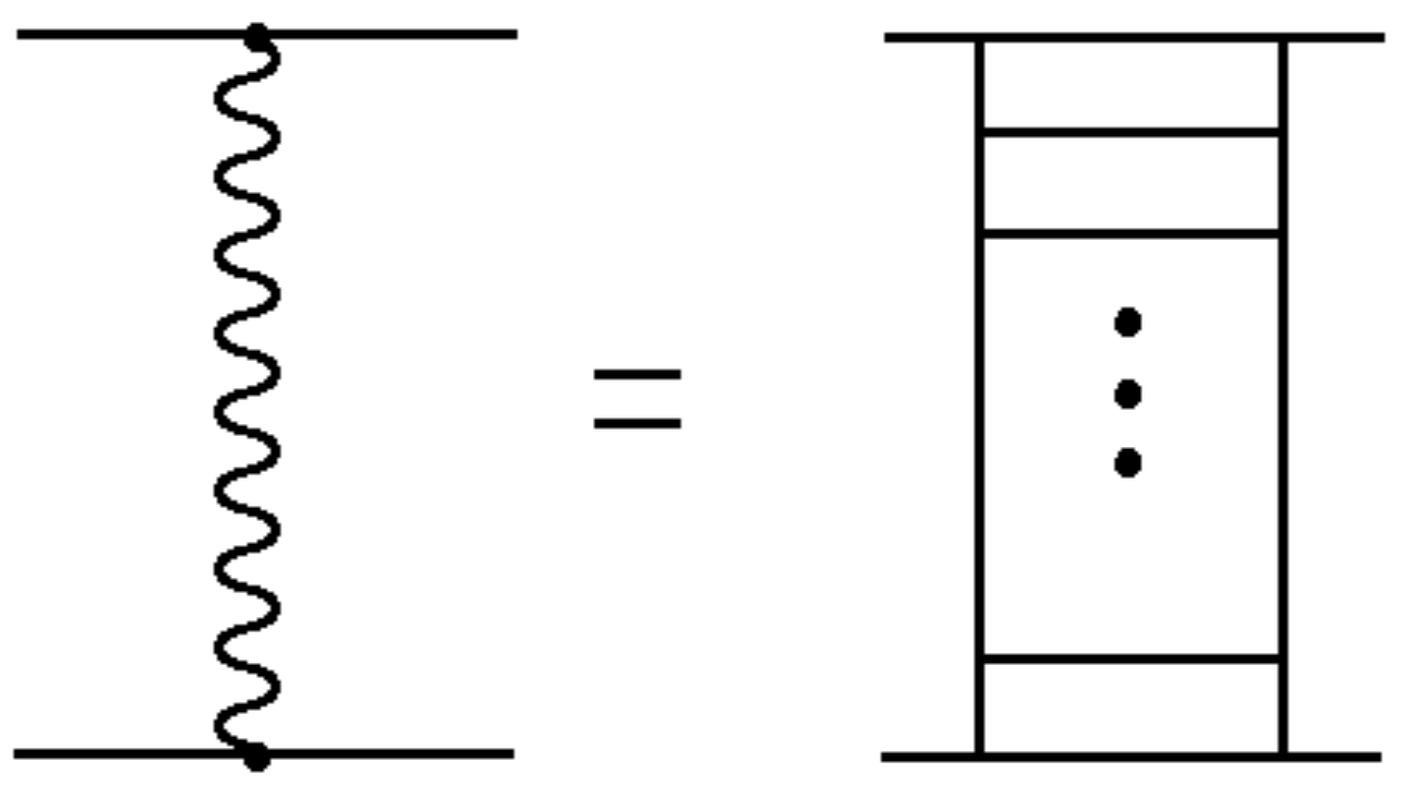
The amplitudes of the one-reggeon exchange, $i{D}_j\left(s_j{k}_j^{\perp 2}\right)$, where $k_j^{\perp 2}$ is the perpendicular part of the square of the transferred reggeon momentum, we will present in the form of the simplest multi-peripheral diagram, as shown in Figure 2. Phase volume of the two-reggeon branching is as follows:

$$d{\mathsf{\Omega }}_2=2{\left(2\pi \right)}^2\delta \left(\overrightarrow{Q}-{\overrightarrow{k}}_1^{\perp }-{\overrightarrow{k}}_2^{\perp }\right)\frac{d^2{k}_1^{\perp }}{2{\left(2\pi \right)}^2}\frac{d^2{k}_2^{\perp }}{2{\left(2\pi \right)}^2},$$

where $\overrightarrow{Q}$ is the transverse part of the total transferred four-momentum $p_a-{p^{\prime }}_a$.

Let us consider the inelastic processes corresponding to the exchange of one or more reggeons. We apply the generalized Cutkosky unitarity bound [7], which defines the imaginary part of any Feynman diagram as the sum of contributions:

$$\mathrm{Im}A\left(s,t\right)=\frac{1}{2i}{\displaystyle \sum _c{\delta }_c}A\left(s,t\right)=\frac{1}{2}{\displaystyle \int d{\tau }_{nc}}A\left(2\to n_c\right)A\left(n_c\to 2\right),$$

(3)

of all sorts of cuttings along some line to the associated amplitudes, the left $A\left(2\to n_c\right)$ and the right $A\left(n_c\to 2\right)=A^{*}\left(2\to n_c\right)$. The discontinuity ${\delta }_{c}A\left(s,t\right)$ along s in the cutting is associated with the production of the state $c$, $d{\tau }_{nc}$ is the partial phase volume, and $n_c$ is the number of lines in the diagram cut by the contour $c$ and displayed on a mass surface. The summation in Equation (3) runs over all admissible cuttings. Since the contribution of any reggeon diagram is a convergent sum of the inputs of Feynman diagrams, the generalized Cutkosky unitarity bound can be directly applied to any reggeon diagram. It can be shown that the cutting line of a one-reggeon amplitude inside the reggeon diagram should run along the entire reggeon, or not to cut it at all.

For the amplitude of the two-reggeon scattering, the absorption parts of the reggeon diagram can be of the following three types:

1)

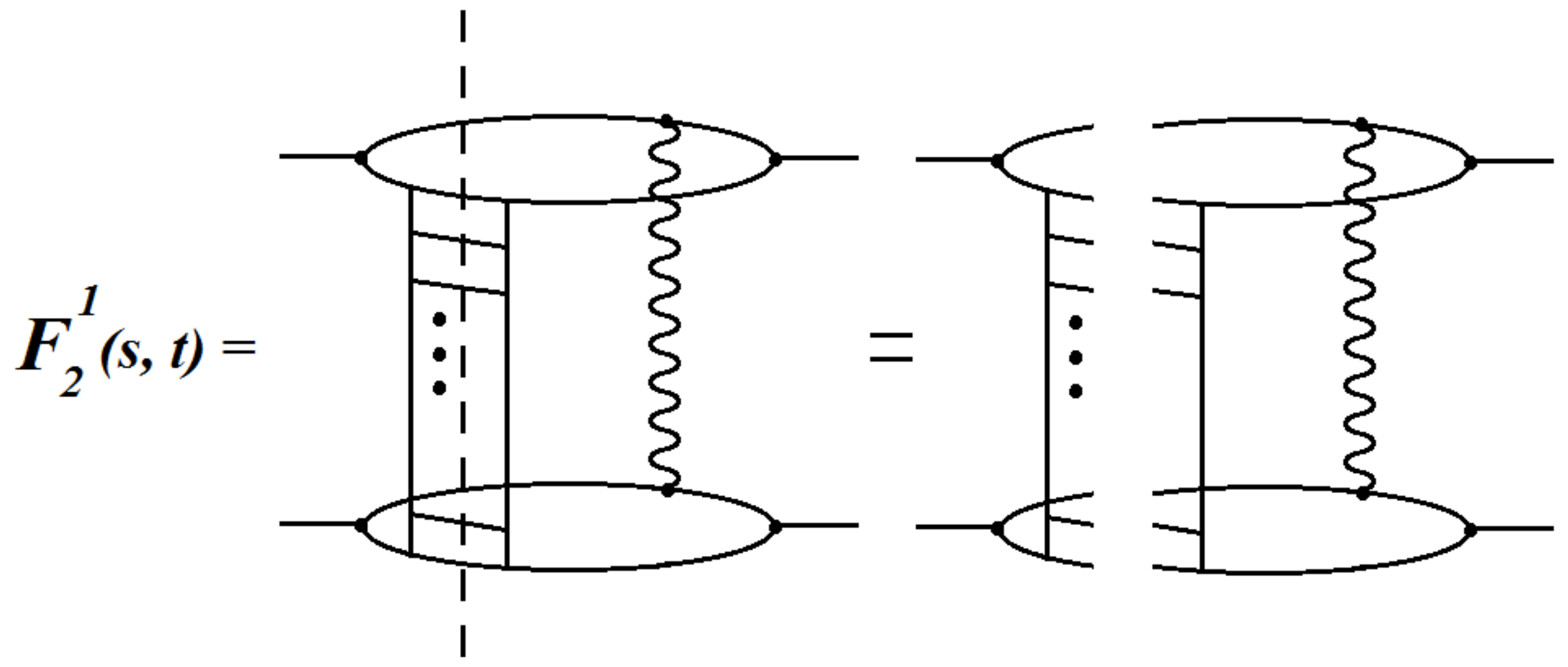
The cutting line is drawn between the reggeons (Figure 3). This corresponds to the process of diffraction dissociation of projectile particles. The absorption part $F_2^0$ is equal to:

$$\begin{array}{cc}\hfill F_2^0\left(s,t\right)=& s{\displaystyle \int d{x}_{1}d{x}_2\delta \left(1-x_1-x_2\right)d{x^{\prime }}_1}d{x^{\prime }}_2\delta \left(1-{x^{\prime }}_1-{x^{\prime }}_2\right)w\left(x_1,x_2\right)w\left({x^{\prime }}_1,{x^{\prime }}_2\right)\hfill \\ & \times {{\displaystyle \int d\mathsf{\Omega }}}_2\left\{\left[i{D}_1\left(s_1,k_1^{\perp 2}\right)\right]{\left[i{D}_2\left(s_2,k_2^{\perp 2}\right)\right]}^{*}+\left[i{D}_2\left(s_2,k_2^{\perp 2}\right)\right]{\left[i{D}_1\left(s_1,k_1^{\perp 2}\right)\right]}^{*}\right\}.\hfill \end{array}$$

(4)

The two terms in the integrand correspond to two possible positions of reggeons in relation to the cutting line.

2)

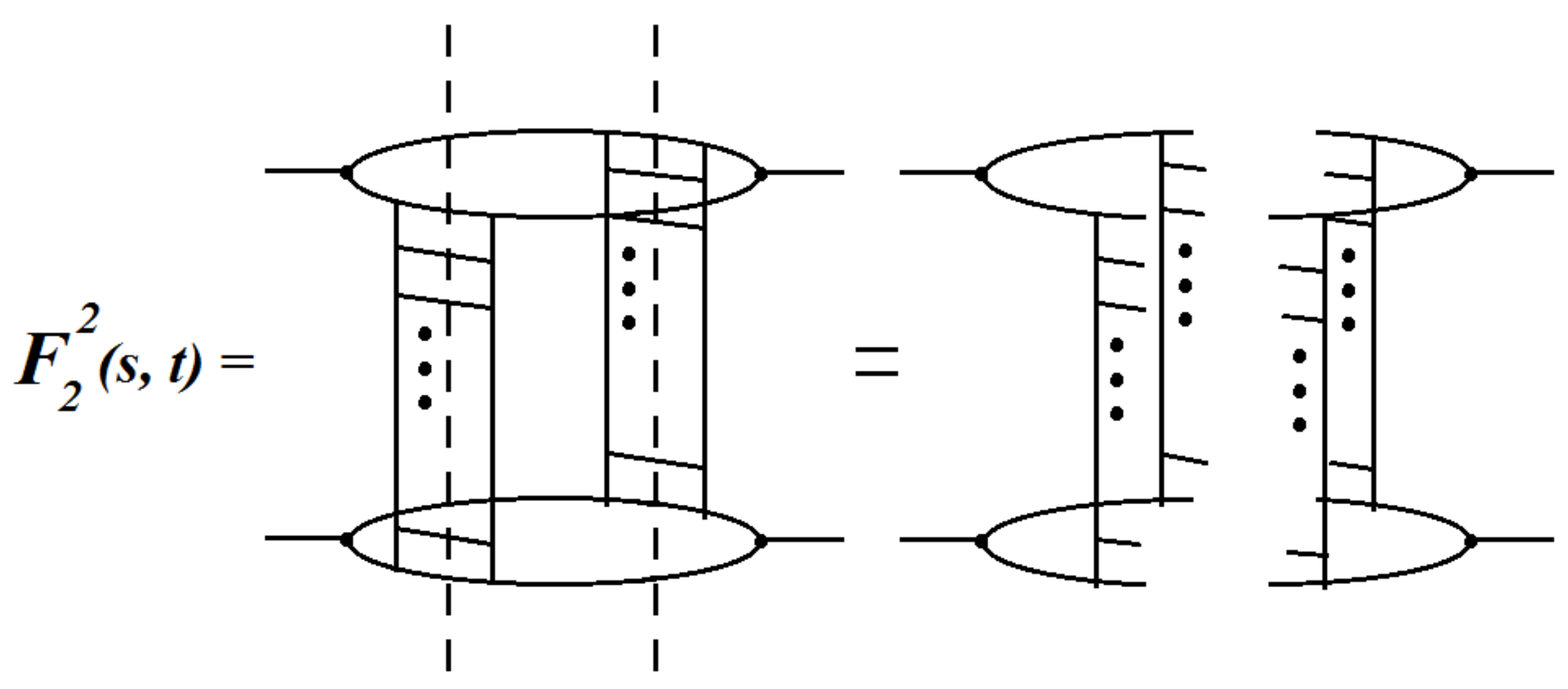
The cutting line is drawn along one of the reggeons (Figure 4). This is a contribution from the interference of the amplitude of the formation of a multi-peripheral particle comb and the same comb with an additional exchange of reggeon. The equation for the absorption part $F_2^1$ looks like:

$$\begin{array}{cc}\hfill F_2^1\left(s,t\right)=& s{\displaystyle \int d{x}_{1}d{x}_2\delta \left(1-x_1-x_2\right)d{x^{\prime }}_1}d{x^{\prime }}_2\delta \left(1-{x^{\prime }}_1-{x^{\prime }}_2\right)w\left(x_1,x_2\right)w\left({x^{\prime }}_1,{x^{\prime }}_2\right)\hfill \\ & \times {{\displaystyle \int d\mathsf{\Omega }}}_2\{\left[i{D}_1\left(s_1,k_1^{\perp 2}\right)\right]\left[2\mathrm{Im}{D}_2\left(s_2,k_2^{\perp 2}\right)\right]+\left[2\mathrm{Im}{D}_2\left(s_2,k_2^{\perp 2}\right)\right]{\left[i{D}_1\left(s_1,k_1^{\perp 2}\right)\right]}^{*}\hfill \\ & +\left[2\mathrm{Im}{D}_1\left(s_1,k_1^{\perp 2}\right)\right]{\left[i{D}_2\left(s_2,k_2^{\perp 2}\right)\right]}^{*}+\left[i{D}_2\left(s_2,k_2^{\perp 2}\right)\right]\left[2\mathrm{Im}{D}_1\left(s_1,k_1^{\perp 2}\right)\right]\}.\hfill \end{array}$$

(5)

Here, the first two terms correspond to the cut reggeon $D_2$ and the position of the reggeon $D_1$ to the left and to the right of the cutting line, and the last two terms correspond to the reggeon cut $D_1$ and the position of the reggeon $D_2$ to the left and to the right of the cutting line.

3)

The cut line is drawn simultaneously on both reggeons (Figure 5). This cutting corresponds to the formation of two multi-peripheral combs. The corresponding absorption part $F_2^2$ is represented as:

$$\begin{array}{cc}\hfill F_2^2\left(s,t\right)=& s{\displaystyle \int d{x}_{1}d{x}_2\delta \left(1-x_1-x_2\right)d{x^{\prime }}_1}d{x^{\prime }}_2\delta \left(1-{x^{\prime }}_1-{x^{\prime }}_2\right)w\left(x_1,x_2\right)w\left({x^{\prime }}_1,{x^{\prime }}_2\right)\hfill \\ & \times {{\displaystyle \int d\mathsf{\Omega }}}_2\left[2\mathrm{Im}{D}_1\left(s_1,k_1^{\perp 2}\right)\right]\left[2\mathrm{Im}{D}_2\left(s_2,k_2^{\perp 2}\right)\right].\hfill \end{array}$$

(6)

Both reggeons are cut here.

Adding these three absorption parts, we obtain the doubled imaginary part of the amplitude of the two-reggeon branching:

$$\begin{array}{cc}\hfill 2\mathrm{Im}A\left(s,t\right)& =2s{\displaystyle \int d{x}_{1}d{x}_2\delta \left(1-x_1-x_2\right)d{x^{\prime }}_1}d{x^{\prime }}_2\delta \left(1-{x^{\prime }}_1-{x^{\prime }}_2\right)w\left(x_1,x_2\right)w\left({x^{\prime }}_1,{x^{\prime }}_2\right)\hfill \\ & \times {{\displaystyle \int d\mathsf{\Omega }}}_2\left[\mathrm{Re}{D}_1\left(s_1,k_1^{\perp 2}\right)\mathrm{Re}{D}_2\left(s_2,k_2^{\perp 2}\right)-\mathrm{Im}{D}_1\left(s_1,k_1^{\perp 2}\right)\mathrm{Im}{D}_2\left(s_2,k_2^{\perp 2}\right)\right].\hfill \end{array}$$

(7)

Similarly, for the absorption parts of the amplitudes with a cutting of $m$ from $n$ reggeons:

$$\begin{array}{cc}{F}_n^m\left(s,t\right)=& {\left(-1\right)}^{n-m}{C}_n^{m}s{\displaystyle \int d{x}_1\dots d{x}_n\delta \left(1-{\displaystyle \sum _1^n{x}_j}\right)d{x^{\prime }}_1}\dots d{x^{\prime }}_n\delta \left(1-{\displaystyle \sum _1^n{x^{\prime }}_j}\right)w\left(x_1,\dots ,x_n\right)w\left({x^{\prime }}_1,\dots ,{x^{\prime }}_n\right)\hfill \\ & \times {{\displaystyle \int d\mathsf{\Omega }}}_n{\displaystyle \prod _{j=1}^{n}2\mathrm{Im}{D}_j\left(s_j,k_j^{\perp 2}\right)}.\hfill \end{array}$$

(8)

From Equation (8), the next relations follow:

$$\begin{array}{l}{\displaystyle \sum _{m=1}^{n}m{F}_n^m\left(s,t\right)}=0,\\ \dots \dots \dots \\ {\displaystyle \sum _{m=l}^{n}m\left(m-1\right)\dots \left(m-l+1\right)F_n^m\left(s,t\right)}=0.\end{array}$$

(9)

These AGK relations were derived for hadron physics. The significant distances are determined by the functions $w\left(x_1,\dots x_n\right)$ and, in order of magnitude, are equal to ${10}^{-15}$ m. In the Appendix, we present a more general proof of the AGK theorem, which will not fix the distance. The proof comes from the unitarity of the $S$-matrix. It proves the theorem not only for the case of elastic scattering but also for any number of initial states. Therefore, it turned out that the theorem is valid for all particles with different energies surrounding a black hole.

The standard scheme for constructing a theory is as follows. The external field is chosen so that it is absent in the distant past and the distant future. In these in- and out-areas, it is possible to unambiguously determine the state of the particle and vacuum. As a result of the action of the external field in the process of evolution of the system in the initial vacuum state, the production of particles starts, so that the result of the evolution of the state corresponding to the in-vacuum does not coincide with the out-vacuum state. Complete information about the processes of particle production, scattering, and annihilation is contained in a unitary operator connecting the in- and out- states, which is called the $S$-matrix.

The applicability of the $S$-matrix theory to the black hole radiation problem was shown in [8]. Let us consider the simplest process of absorption of a charged particle (proton) by a black hole. At the initial time, the particle is sufficiently distant from the black hole, so that its interaction is negligible. This allows the establishment of an in-state, including a particle and a black hole. Subsequently, the particle is attracted to a black hole, increasing its momentum and energy. From a certain moment, the particle begins to emit photons in a bremsstrahlung, dumping a part of the energy received from a black hole.

We cannot “turn off” the gravitational field of a black hole. As the particle approaches it, the interaction will increase. The resulting state is a black hole, a particle, and photons will not be an out-state. However, according to this state, we perform the convolution of the T-matrices in the unitarity bound. So, we get diagrams in which there will be free particles in the initial and final states.

It should be noted that the remote observer will be able to register only those photons that fly outside of the Schwarzschild radius. Particles that fall inside the Schwarzschild radius remain “invisible” to an observer. Therefore, we must average on these states. That is, instead of pure quantum-mechanical states, we must research inclusive cross-sections.

2. The Dependence of the Luminosity of a Black Hole on Its Mass

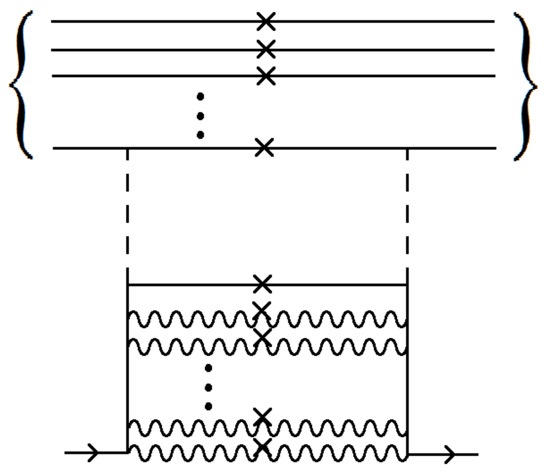
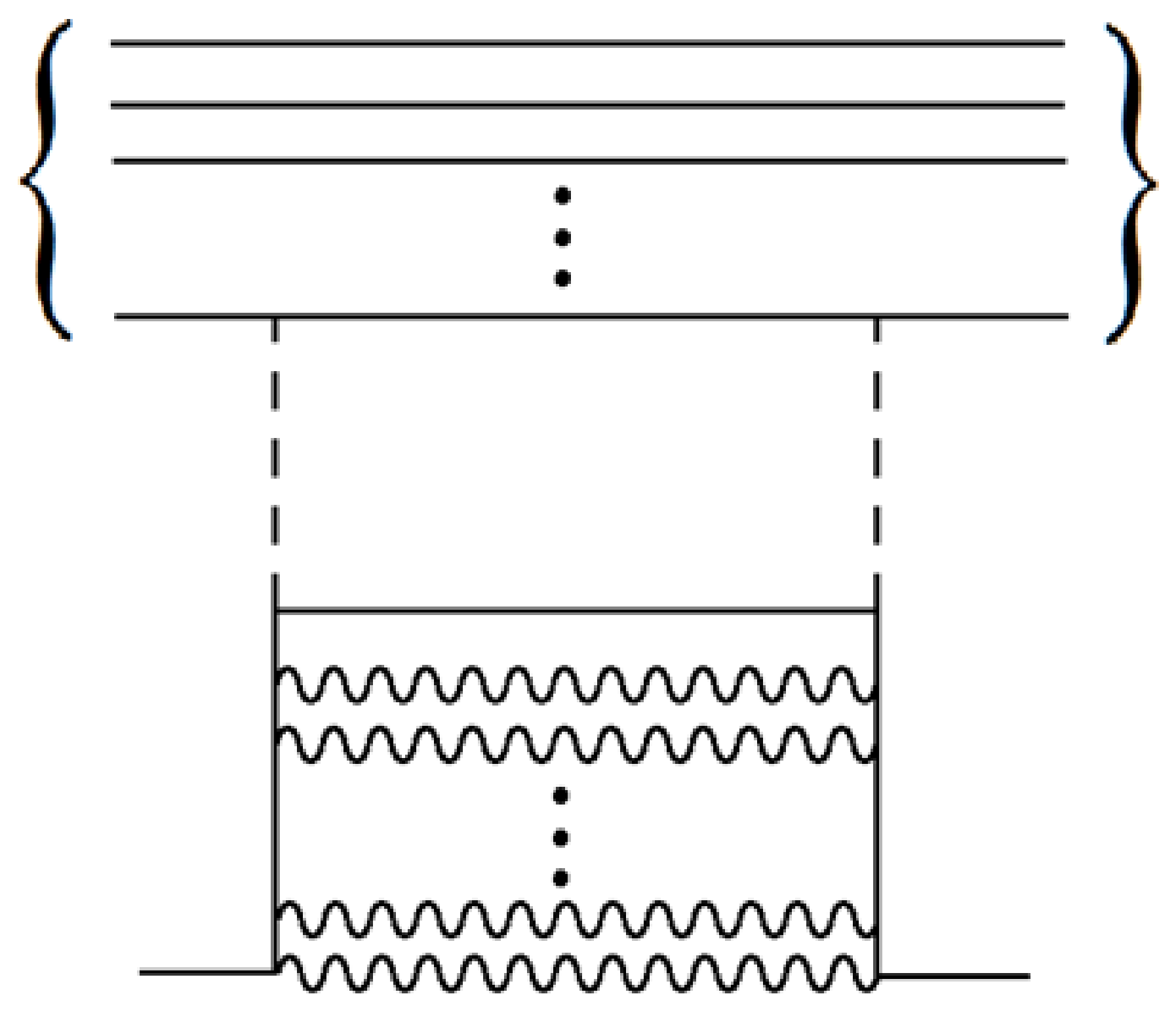
We consider the following picture of the dependence of a black hole on its mass. Let us consider a proton on a long distance from a black hole. As it approaches the black hole, the momentum and energy of this proton increase, and it begins to emit photons in a bremsstrahlung. The corresponding Feynman diagram has the following form (Figure 6). We consider the simplest black hole consisting only of neutrons. A part of the photons and the proton will pass through the Schwarzschild radius, but a certain number of photons will be emitted into the surrounding space. These photons will carry the energy “sucked off” from the black hole. To determine the probabilities of the processes, we have to multiply by the complex conjugate amplitude, as shown in Figure 7.

We get the square of the amplitude modulus corresponding to the exclusive photon emission cross-section in the field of a black hole by a proton. Integrating over the phase volume of all particles, including black hole particles, we obtain the imaginary part of the amplitude of elastic scattering of a proton by a black hole.

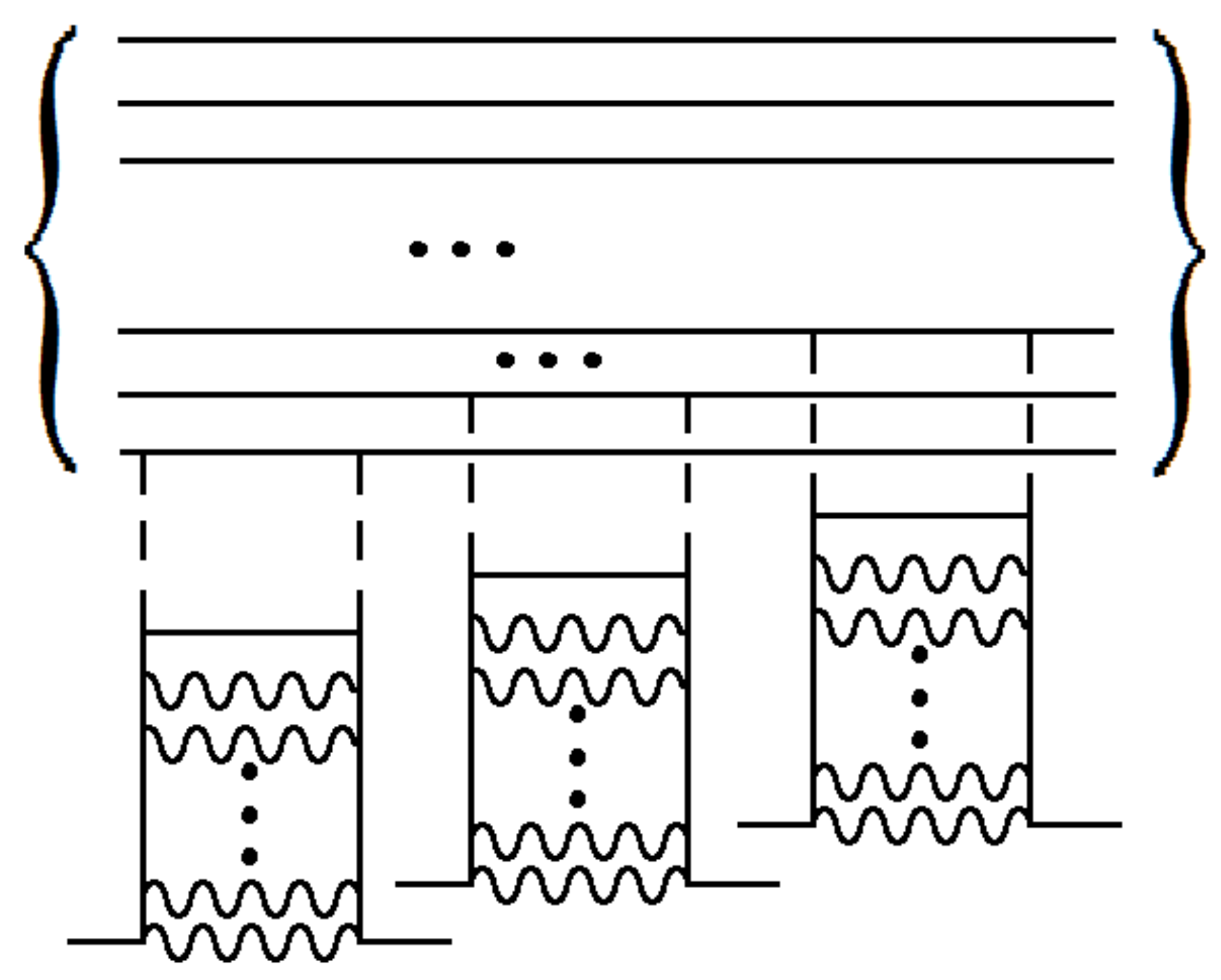
If a black hole attracts several protons, we get the Feynman diagrams in the form of Figure 8.

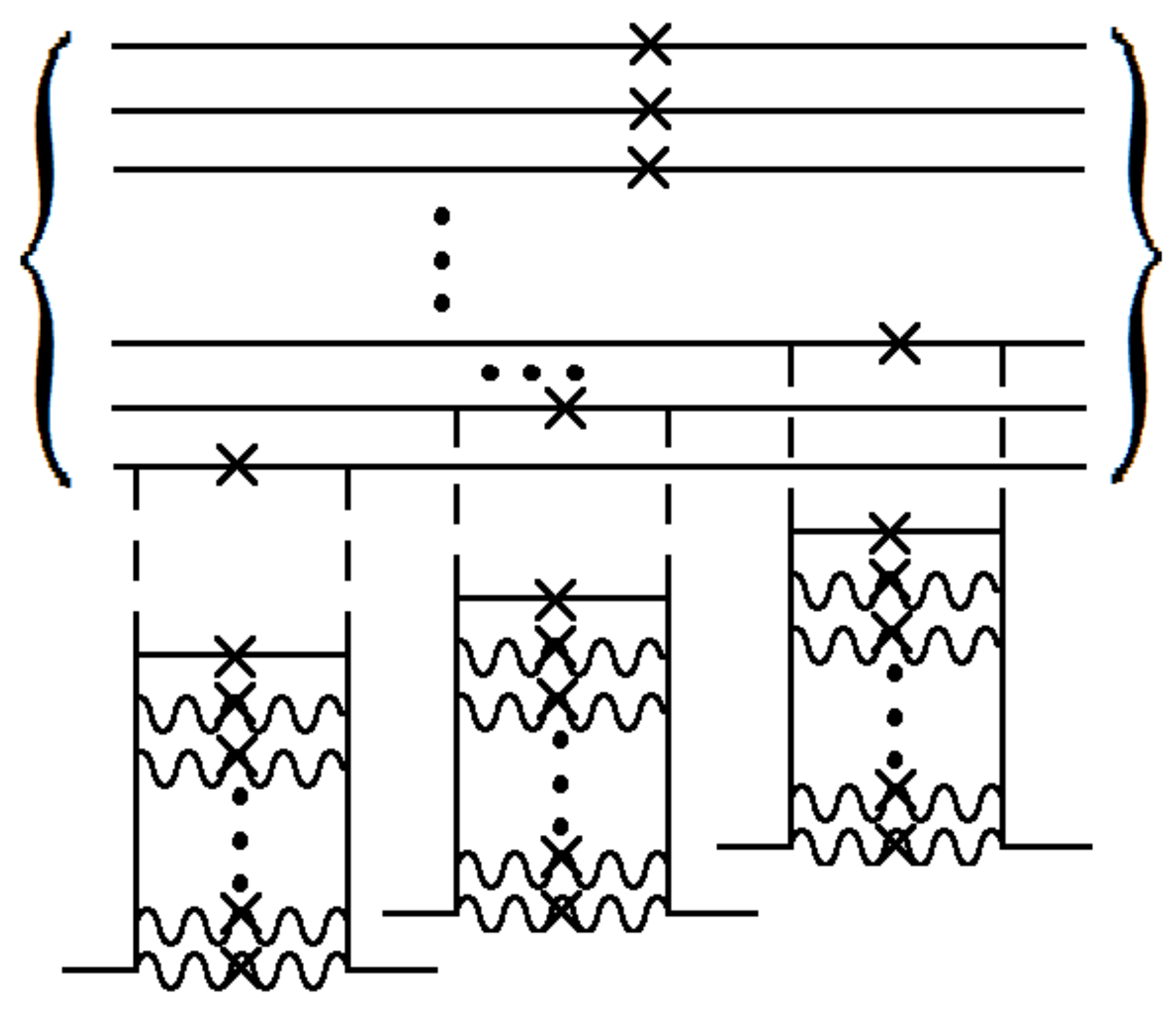
Taking the square of the module of this diagram (Figure 9), we obtain an exclusive cross-section for the production of photons from protons in the field of a black hole. Integrating over the phase volume, we obtain the contribution into the total cross-section of this process.

From the presence of the imaginary parts shown in Figure 7 and Figure 9, it follows that there are full amplitudes corresponding to the elastic scattering of one or several protons on the black hole, as shown in Figure 10 and Figure 11.

In the Appendix it is shown that the AGK theorem is valid for such diagrams.

An averaging is necessary over particles located within the Schwarzschild radius. Such averaging can be carried out using the inclusive technique [9,10,11,12]. The inclusive cross-section is obtained from the cut amplitudes, fixing the observed particle, integrating over the momentum of others, and summing over all the remaining particles. Therefore, for inclusive cross-sections, cuts between amplitudes do not provide any contributions. Equations (A30)–(A39) (see also (9)) imply that all diagrams for single-particle inclusive cross-sections are cut down. Only the diagram such as one shown in Figure 10, remains. Since both gravitons are connected to the same black hole particle, the input of this diagram will be proportional to the sum of all black hole particles, i.e., to the mass of the black hole.

The total energy carried away by the emitted particle is equal to the energy of the particle multiplied by the inclusive cross-section of the production of such a particle and integrated over all possible energy values. The luminosity is proportional to the energy carried away by a photon in a certain frequency range of the photon. It can be determined as follows:

$$L\propto {\displaystyle \underset{w_1}{\overset{w_2}{\int }}\frac{dw}{w}}{\displaystyle \int d^2{k}_{\perp }\cdot wf\left(w,k_{\perp }^2\right)},$$

(10)

where $f\left(w,k_{\perp }^2\right)$ is the inclusive cross-section of the photon radiation by a proton in the field of a black hole. Considering that:

$$f\left(w,k_{\perp }^2\right)\propto M_{BH},$$

we will have for luminosity:

$$L=a{M}_{BH},$$

where the parameter $a$ depends only on the amplitude of the graviton proton scattering.

3. Comparison with Experimental Data

The data are found to provide the dependence of the black hole mass on the black hole luminosity such as [1]:

$${\log }_{10}{M}_{BH}=\left(8.95\pm 0.11\right)+\left(1.11\pm 0.18\right){\log }_{10}\left(L_V/{10}^{11}\right),$$

(11)

and [2]:

$${\log }_{10}{M}_{BH}=9.16+1.16{\log }_{10}\left(L_V/{10}^{11}\right).$$

(12)

This goes along with the correspondences:

$$\begin{array}{l}{L}_V=0.87\cdot {10}^3{M}_{BH}^{0.9},\\ L_V=1.27\cdot {10}^3{M}_{BH}^{0.86}.\end{array}$$

(13)

Such correspondences are very close to the one we obtained (1). In [2], it is also noted that the black holes of the galaxies NGC 3842 and NGC4889 do not fit into the phenomenological formulas that describe the black holes given in Table 4 of [2].

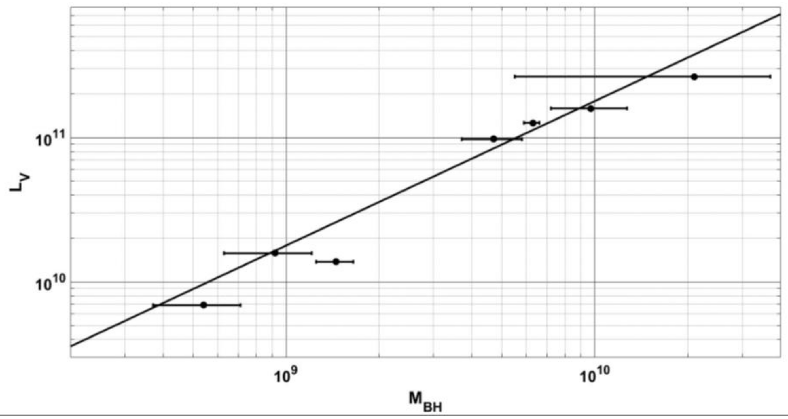
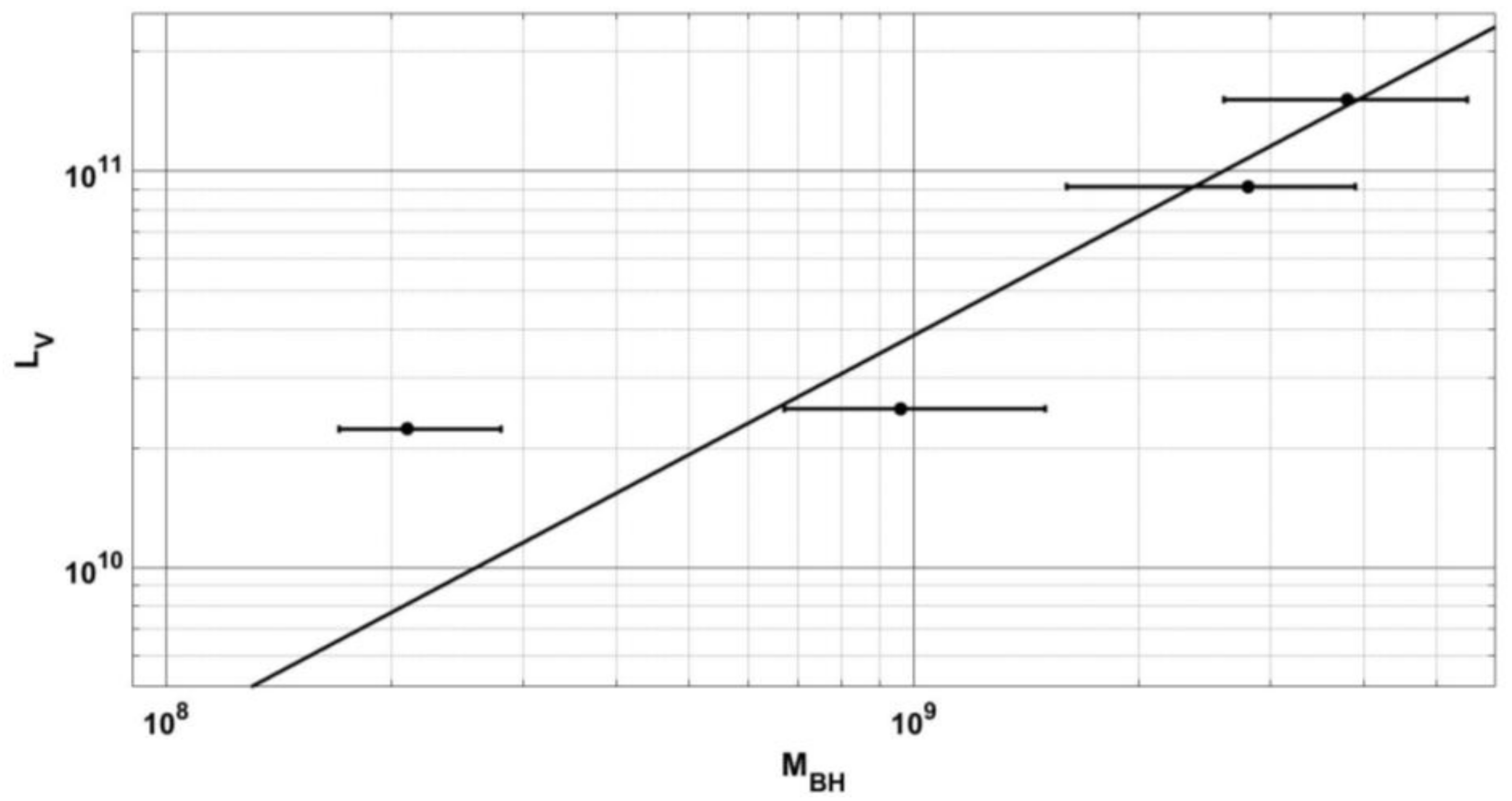
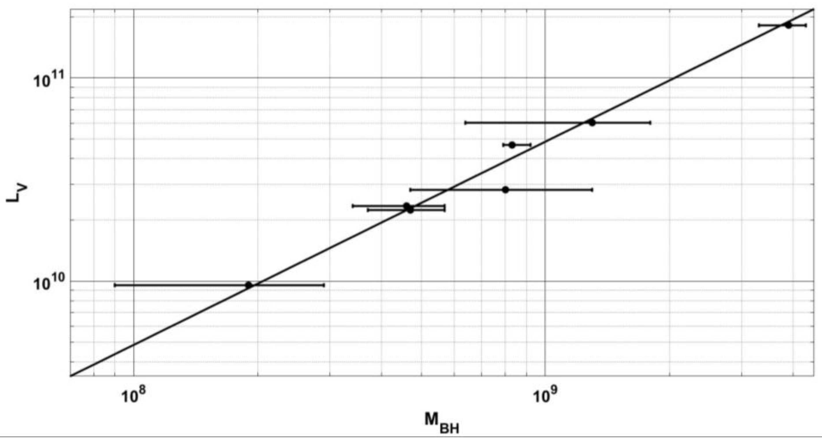
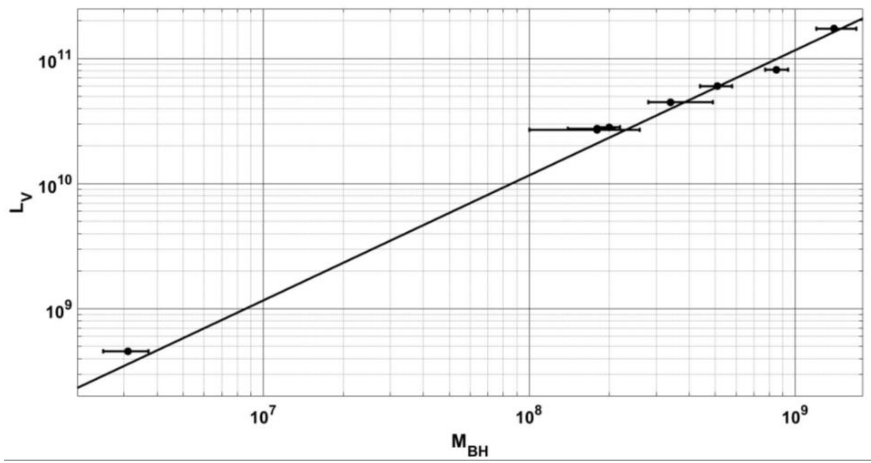
Using the quantum mechanical formula derived by us, we divided the data [2] into five groups as given in

Table 1. The first group of galaxies [2]: $L_V/M_{BH}<25$.

Galaxy	${\mathit{M}}_{\mathit{B}\mathit{H}}$	${\mathit{M}}_{\mathit{B}\mathit{H}\mathbf{min}}$	${\mathit{M}}_{\mathit{B}\mathit{H}\mathbf{max}}$	${\mathbf{log}}_{10}{\mathit{L}}_{\mathit{V}}$	${\mathit{L}}_{\mathit{V}}/{\mathit{M}}_{\mathit{B}\mathit{H}}$
N4889	2.1 × 1010	5.5 × 109	3.7 × 1010	11.42	12.5
N3842	9.7 × 109	7.2 × 109	1.27 × 1010	11.20	16.3
N4486 (M87)	6.3 × 109	5.9 × 109	6.6 × 109	11.10	20.0
N4649 (M60)	4.7 × 109	3.7 × 109	5.8 × 109	10.99	21.2
N1332	1.45 × 109	1.25 × 109	1.65 × 109	10.14	9.5
N4291	9.2 × 108	6.3 × 108	1.21 × 109	10.20	17.2
N5845	5.4 × 108	3.7 × 108	7.1 × 109	9.84	12.8

,

Table 2. The second group of galaxies [2]: $25<L_V/M_{BH}<40$.

Galaxy	${\mathit{M}}_{\mathit{B}\mathit{H}}$	${\mathit{M}}_{\mathit{B}\mathit{H}\mathbf{min}}$	${\mathit{M}}_{\mathit{B}\mathit{H}\mathbf{max}}$	${\mathbf{log}}_{10}{\mathit{L}}_{\mathit{V}}$	${\mathit{L}}_{\mathit{V}}/{\mathit{M}}_{\mathit{B}\mathit{H}}$
N6086	3.8 × 109	2.6 × 109	5.5 × 109	11.18	39.7
IC1459	2.8 × 109	1.6 × 109	3.9 × 109	10.96	35.8
N3115	9.6 × 108	6.7 × 108	1.5 × 109	10.40	26.1
N4026	2.1× 108	1.7 × 108	2.8 × 108	10.35	34.5

,

Table 3. The third group of galaxies [2]: $90<L_V/M_{BH}<150$.

Galaxy	${\mathit{M}}_{\mathit{B}\mathit{H}}$	${\mathit{M}}_{\mathit{B}\mathit{H}\mathbf{min}}$	${\mathit{M}}_{\mathit{B}\mathit{H}\mathbf{max}}$	${\mathbf{log}}_{10}{\mathit{L}}_{\mathit{V}}$	${\mathit{L}}_{\mathit{V}}/{\mathit{M}}_{\mathit{B}\mathit{H}}$
A1836-BCG	3.9 × 109	3.3 × 109	4.3 × 109	11.26	47
N1399	1.3 × 109	6.4 × 108	1.8 × 109	10.78	46
N524	8.3 × 108	7.9 × 108	9.2 × 108	10.67	56
N3608	4.7 × 108	3.7 × 108	5.7 × 108	10.35	47.8
N3379(M105)	4.6 × 108	3.4 × 108	5.7 × 108	10.37	50.9
N3377	1.9 × 108	9.0 × 107	2.9 × 108	9.98	50.3

,

Table 4. The fourth group of galaxies [2]: $90<L_V/M_{BH}<150$.

Galaxy	${\mathit{M}}_{\mathit{B}\mathit{H}}$	${\mathit{M}}_{\mathit{B}\mathit{H}\mathbf{min}}$	${\mathit{M}}_{\mathit{B}\mathit{H}\mathbf{max}}$	${\mathbf{log}}_{10}{\mathit{L}}_{\mathit{V}}$	${\mathit{L}}_{\mathit{V}}/{\mathit{M}}_{\mathit{B}\mathit{H}}$
A3565-BCG	1.4 × 109	1.2 × 109	1.7 × 109	11.24	124
N4374 (M84)	8.5 × 108	7.7 × 108	9.4 × 108	10.91	96.4
N1399	5.1 × 108	4.4 × 108	5.8 × 108	10.78	118
N3585	3.4 × 108	2.8 × 108	4.9 × 108	10.65	131
N4697	2.0 × 108	1.8 × 108	2.2 × 108	10.45	141
N5576	1.8 × 108	1.4 × 108	2.1 × 108	10.44	143
N821	1.8 × 108	1.0 × 108	2.6 × 108	10.43	149
N221 (M32)	3.1 × 106	2.5 × 106	3.7 × 106	8.66	147

and

Table 5. The fifth group of galaxies [2]: $150<L_V/M_{BH}<350$.

Galaxy	${\mathit{M}}_{\mathit{B}\mathit{H}}$	${\mathit{M}}_{\mathit{B}\mathit{H}\mathbf{min}}$	${\mathit{M}}_{\mathit{B}\mathit{H}\mathbf{max}}$	${\mathbf{log}}_{10}{\mathit{L}}_{\mathit{V}}$	${\mathit{L}}_{\mathit{V}}/{\mathit{M}}_{\mathit{B}\mathit{H}}$
N4261	5.5 × 108	4.3 × 108	6.6 × 108	11.02	190
N7052	4.0 × 108	2.4 × 108	6.8 × 108	10.87	185
N5128	3.0 × 108	2.8 × 108	3.4 × 108	10.66	152
N4473	1.0 × 108	5.0 × 107	1.5 × 108	10.39	245
N4459	7.4 × 107	6.0 × 107	8.8 × 107	10.36	310
N1023	4.6 × 107	4.1 × 107	5.1 × 107	10.18	330
N2549	1.4 × 107	1.0 × 107	1.47 × 107	9.6	284
N4486A	1.3 × 107	9.0 × 106	1.8 × 107	9.41	198
N4757	1.0 × 107	4.0 × 106	1.6 × 107	9.42	263

and shown in Figure 12, Figure 13, Figure 14, Figure 15 and Figure 16 along with the dependence (1).

We believe that the substance of the universe consists of 91% of hydrogen and 9% of helium. We have considered only one charged particle. In reality, hydrogen and helium atoms fall on a black hole. In hydrogen, there are two charged particles: a proton and an electron. In helium, there are four charged particles and two neutrons. Therefore, we must take into account the bremsstrahlung of all these particles together.

We can assume that the first group includes galaxies in which the substance is distributed around a black hole, like in the whole Universe. Therefore, galaxies NGC3842 and NGC4889 do not differ from other galaxies. In other groups, the density of the substance near the black hole is increased. Assuming that the remaining parameters of the graviton-proton interaction are the same for all groups, then the substance density is increased by two, three, six, and ten times. However, in this matter, more studies are required, which are planned for the future.

4. Conclusions

It was shown a black hole can emit photons via a mechanism of Beckenstein—Hawking radiation [13,14,15,16]. In this paper, we made the case that there is another possible process for emitting photons from a black hole.

We obtained a linear dependence of the luminosity of a black hole on the mass of a black hole. It occurs because all inelastic processes of photon emission by several atoms falling on a black hole are completely cut down by interference. Only the inclusive amplitude of photon emission by one atom falling on a black hole remains. The quantum mechanical formula we derived actually coincides with the phenomenological formulas described earlier in other papers. We believe that the difference in the constant of proportionality in (1) is due to differences in the density of substance near the black hole.

We also believe that the dependence of the galaxy velocity dispersion $\sigma$ on the mass of the black hole:

$$\left(\sigma /km{s}^{-1}\right)=4.8\cdot M_{BH}^{0.2},$$

most likely cannot be derived from a quantum-mechanical consideration.

References

- Gültekin, K.; Richstone, D.O.; Gebhardt, K.; Lauer, T.R.; Tremaine, S.; Aller, M.C.; Bender, R.; Dressler, A.; Faber, S.M.; Filippenko, A.V.; et al. The M-σ and M-L Relations in Galactic Bulges, and Determinations of their Intrinsic Scatter. Astrophys. J. 2009, 698, 198–221. [Google Scholar] [CrossRef]
- McConnell, N.J.; Ma, C.P.; Gebhardt, K.; Wright, S.A.; Murphy, J.D.; Lauer, T.R.; Graham, J.R.; Richstone, D.O. Two ten-billion-solar-mass black holes at the centres of giant elliptical galaxies. Nature 2011, 480, 215–218. [Google Scholar] [CrossRef] [PubMed] [Green Version]
- Gültekin, K.; Barth, A.; Gebhardt, K.; Greene, J.; Ho, L.; Juneau, S.; Ma, C.P.; Seth, A.; Valluri, M.; Walsh, J. Astro2020 Science White Paper: Black Holes Across Cosmic Time. arXiv 2019, arXiv:1904.01447. [Google Scholar]
- Abramovskii, V.A.; Kancheli, O.V.; Gribov, V.N. Structure of inclusive spectra and fluctuations in inelastic processes caused by multiple-pomeron exchange. eConf 1972, 720906, 389–413. [Google Scholar]
- Abramovsky, V.A.; Gribov, V.N.; Kancheli, O.V. Character of Inclusive Spectra and Fluctuations Produced in Inelastic Processes by Multi-Pomeron Exchange. Yad. Fiz. 1974, 18, 595–616. (in Russian); English translation: Sov. J. Nucl. Phys. 1974, 18, 308–317. [Google Scholar]
- Abramovsky, V.A.; Leptoukh, G.G. The AGK rules revised. Sov. J. Nucl. Phys. 1992, 55, 903–905. [Google Scholar]
- Cutkosky, R.E. Singularities and discontinuities of Feynman amplitudes. J. Math. Phys. 1960, 1, 429–433. [Google Scholar] [CrossRef]
- Novikov, I.D.; Frolov, V.P. Physics of Black Holes; Kluwer Academic: Dordrecht, The Netherlands, 1989. [Google Scholar]
- Feynman, R.P. Very high-energy collisions of hadrons. Phys. Rev. Lett. 1969, 23, 1415–1417. [Google Scholar] [CrossRef]
- Mueller, A.M. O(2,1) Analysis of Single-Particle Spectra at High Energy. Phys. Rev. D 1970, 2, 2963–2969. [Google Scholar] [CrossRef]
- Kancheli, O.V. Inelastic differential cross sections at high energies and duality. Pisma Zh. Eksp. Teor. Fiz. 1970, 11, 397–400. (in Russian); English translation: JETP Lett. 1970, 11, 267–270. [Google Scholar]
- Abramovsky, V.A.; Kancheli, O.V.; Mandzhavidze, I.D. Total differential cross-sections of inelastic processes at high energies. Yad. Fiz. 1971, 13, 1102–1115. (in Russian); English translation: Sov. J. Nucl. Phys. 1971, 13, 630. [Google Scholar]
- Beckenstein, J.D. Black holes and the second law. Nuovo Cim. Lett. 1972, 4, 737–740. [Google Scholar] [CrossRef]
- Beckenstein, J.D. Black holes and entropy. Phys. Rev. D 1973, 7, 2333–2346. [Google Scholar] [CrossRef]
- Hawking, S.W. Black hole explosions? Nature 1974, 248, 30–31. [Google Scholar] [CrossRef]
- Hawking, S.W. Particle creation by black holes. Commun. Math. Phys. 1975, 43, 199–220. [Google Scholar] [CrossRef]
- Mandelstam, S. Cuts in the Angular-Momentum Plane. Nuovo Cim. 1963, 30, 1148–1162. [Google Scholar] [CrossRef]
Figure 1.
The simplest amplitude diagram of a two-reggeon branching in the interaction of two hadrons with four-momenta pa and pb. The wavy lines designate reggeons, and the solid lines denote scalar particles. See text for more details.
Figure 2.
The simplest model of a reggeon. The lines are as in Figure 1.
Figure 3.
Cut of the double reggeon diagram between the reggeons. The lines are as in Figure 1.
Figure 4.
Cut along one of the reggeons. The lines are as in Figure 1.
Figure 5.
Cut along both reggeons. The lines are as in Figure 1.
Figure 6.
The amplitude of absorption of a proton by a black hole. Solid lines in curly brackets denote the protons inside the black hole. Wavy lines represent photons.
Figure 7.
Square of the modulus of the absorption amplitude of a proton by a black hole. The lines are as in Figure 6.
Figure 8.
Absorption amplitude of several protons by a black hole. The lines are as in Figure 6
Figure 9.
Squared modulus of the amplitude of the absorption of several protons by a black hole. The lines are as in Figure 6.
Figure 10.
The elastic scattering amplitude of a proton on a black hole. The lines are as in Figure 6.
Figure 11.
The elastic scattering amplitude of several protons on a black hole. The lines are as in Figure 6.
Figure 12.
Dependence of the luminosity of a black hole on its mass (Table 1). The data are taken from [2]. .
Figure 13.
Figure 13. Dependence of the luminosity of a black hole on its mass (Table 2). The data are taken from [2]. .
Figure 14.
Dependence of the luminosity of a black hole on its mass (Table 3). The data are taken from [2]. .
Figure 15.
Dependence of the luminosity of a black hole on its mass (Table 4). The data are taken from [2]. .
Figure 16.
Dependence of the luminosity of a black hole on its mass (Table 5). The data are taken from [2]. .