Covid-19 Predictions Using a Gauss Model, Based on Data from April 2 †


1
Department of Chemistry and Applied Biosciences, ETH Zurich, 8093 Zurich, Switzerland
2
Space- and Astrophysics, Ruhr University Bochum, D-44780 Bochum, Germany
3
Institute of Theoretical Physics and Astrophysics, Christian-Albrechts-University Kiel, D-24118 Kiel, Germany
4
Polymer Physics, Department of Materials, ETH Zurich, 8093 Zurich, Switzerland
*
Authors to whom correspondence should be addressed.
†
This manuscript was submitted to the medRxiv preprint server on April 5, and experienced enormous delay afterwards. We decided to send in the original rather than updated manuscript for a fair assessment of its content.
Physics 2020, 2(2), 197-212; https://0-doi-org.brum.beds.ac.uk/10.3390/physics2020013
Submission received: 13 April 2020
/
Revised: 16 May 2020
/
Accepted: 2 June 2020
/
Published: 5 June 2020
(This article belongs to the Special Issue Physics Methods in Coronavirus Pandemic Analysis)
Abstract
:We study a Gauss model (GM), a map from time to the bell-shaped Gaussian function to model the deaths per day and country, as a simple, analytically tractable model to make predictions on the coronavirus epidemic. Justified by the sigmoidal nature of a pandemic, i.e., initial exponential spread to eventual saturation, and an agent-based model, we apply the GM to existing data, as of 2 April 2020, from 25 countries during first corona pandemic wave and study the model’s predictions. We find that logarithmic daily fatalities caused by the coronavirus disease 2019 (Covid-19) are well described by a quadratic function in time. By fitting the data to second order polynomials from a statistical -fit with 95% confidence, we are able to obtain the characteristic parameters of the GM, i.e., a width, peak height, and time of peak, for each country separately, with which we extrapolate to future times to make predictions. We provide evidence that this supposedly oversimplifying model might still have predictive power and use it to forecast the further course of the fatalities caused by Covid-19 per country, including peak number of deaths per day, date of peak, and duration within most deaths occur. While our main goal is to present the general idea of the simple modeling process using GMs, we also describe possible estimates for the number of required respiratory machines and the duration left until the number of infected will be significantly reduced.
1. Introduction
Nowadays, numerous models to predict the spreading of infectious diseases like Covid-19 are available, for example the actively discussed susceptible-infected-removed (SIR) model [1,2,3,4]. Many of these models are either toy models using families of functions [5,6,7,8], machine learning [9,10,11], neural network [12,13], transmission [14,15], growth [16], agent-based [17], or Bayesian regression models [18,19] or they are so complex [4,20], by taking into account a wide range of factors, that simple predictions are not possible [21,22]. In times of the coronavirus epidemic, predictions such as the maximum number of fatalities per day or the date of the peak number of newly seriously sick persons per day (SSPs) are valuable data for governments around the world, especially those facing the beginning of an exponential increase of casualties, and we hope to serve the people in charge with the here presented approach. In particular, fast predictions on the course of the coronavirus disease are crucial for policy makers to optimize their management of the disease wave. To feed into the current debate on infectious disease models, we would like to propose a Gauss model (GM) as a simple, but effective description of fatalities caused by Covid-19 over time, similar to recent studies for the US [23] and for Germany [24]. In contrast to this previous work, we choose to use the logarithm of the reported daily death rates [25], instead of cumulative infections, as monitored input data and we also do not rely on doubling times.
The Gauss model maps time to the bell-shaped Gaussian function to fit existing data of deaths per day and country, and to use this fit to extrapolate the deaths per day to future times. Though the GM may appear too simple to be predictive, we can justify its use by several arguments: (1) the GM appears to be a special case of the SIR model, as recently suggested by a numerical study [26], (2) the GM is compatible with an agent-based epidemological model developed and presented in Appendix A, (3) the GM captures the data available today well, including the entire first epidemic wave in China, (4) epidemics are initially exponential and eventually saturating processes in cumulative quantities and thus give rise to bell-shaped daily quantities. A general ansatz for a sigmoidal time evolution involving a polynomial in the exponent of an exponential shows that coefficients of higher than GM order are not required to capture the existing data—all of which we will explain in detail.
The here explored GM does not present a model capable of similar mechanistic and causal richness compared with some of the existing infectious disease models. Our only addition is to note and use for predictions the macroscopic Gaussian nature of the time evolution of cumulative fatalities that is universal among all countries. The true performance of models and simulations in this pandemic might become clear only months or years from now [27]. Model predictions generally depend on the available data, which changes every day and makes systematic model comparisons challenging. For this reason, we set up a website (https://www.complexfluids.ethz.ch/corona) as part of our Supplementary Information that provides up-to-date data as well as predictions and compares these new predictions to the ones presented in this article based on data from April 2. The Supplementary Information also features GM fits for additional countries not considered in this work.
2. Results
2.1. Gauss Model (GM)
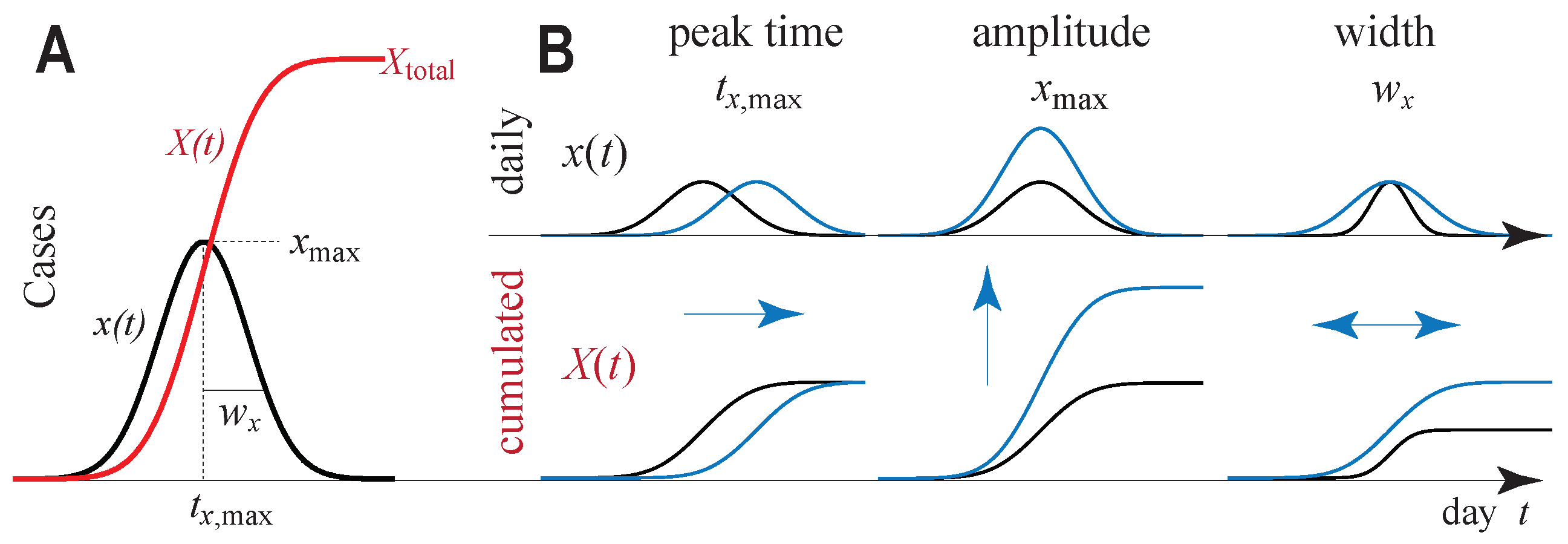
We model the time-dependent daily change of infections and daily change of deaths with their own, a priori independent, time-dependent Gaussian functions denoted by and . Each Gaussianian is a bell-shaped curve, the black line in Figure 1A, characterized by three independent parameters: a width, a maximum height and a time at which the Gaussian curve attains this maximum height. For any value of these parameters, the general form of the Gaussian function—the bell-shaped curve in Figure 1A—is fixed, but the concrete fit to given data can be optimized, as illustrated in Figure 1B for varying parameters.
It must be emphasized that we model the daily change of deaths, in contrast to the cumulative number of deaths, more frequently available in public, because the change of deaths allows for a fit that emphasizes data around the peak time more than marginal data at the beginning or end of the pandemic wave, i.e., the time of interest for predicted quantities. We will explain this point in the discussion. The cumulative deaths are the sum of all previous daily deaths up to today, while the number of daily deaths in turn is the difference of two consecutive days in cumulative deaths. In Figure 1A, the red plot illustrates the cumulative number of deaths as a function of time for the respective daily number of deaths in the same panel.
2.2. Logarithmic Daily Fatalities Are Quadratic
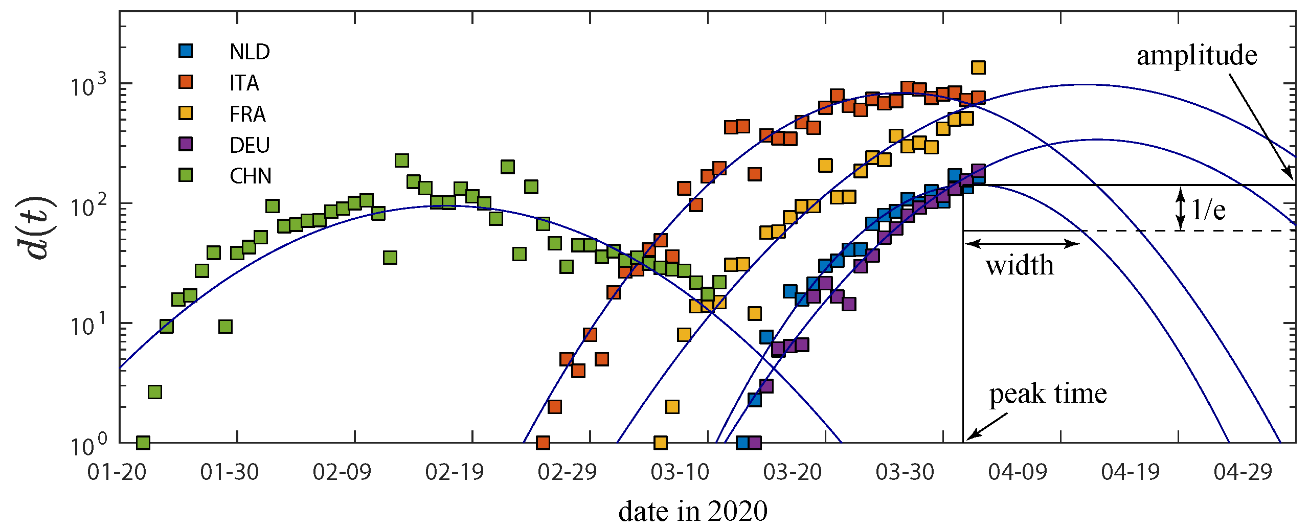
Next, we fit a polynomial of second order to the logarithm of d of 14 countries as a function of time using a -fit. The resulting quadratic fit is plotted in Figure 2. For the remaining 11 countries, similar fits could only be performed for the daily number of infections. It is worthwhile mentioning that we explored the possibility to obtain better fits using higher than second order polynomials, whose coefficient in front of the highest, necessarily even, power must be negative to ensure a sigmoidal cumulative number of fatalities. It turned out that all these higher order coefficients were negligibly small and varied considerably across countries, even taking on positive or negative signs for different countries. We concluded that these higher order coefficients fit more noise than signal. Therefore, we used a second order polynomial (the GM) to fit logarithmic daily deaths. Higher order coefficients might become of relevance for times well after the peak of the first wave of the pandemic, i.e., during times (i) for which predictions about required equipment are of much less relevance, and (ii) that may already be faced with the onset of a second wave.
We prefer to base any quantitative conclusions only on the number of deaths, and not on the number of infections per day. Deaths are better documented than monitored infections in nearly all countries. A death caused by Covid-19 is easier to count than an infection, which might cause no to moderate symptoms and hence might remain uncounted. Statistically, a constant fraction of infected die from Covid-19 at a later time after being registered as infected [27,28]. Thus, infection and death curves are equivalent descriptions of time evolution of Covid-19, and the coefficients characterizing their shape can be expected to be closely related. To demonstrate that infections and deaths follow the GM, we analyzed and show results for both measures.
2.3. The Fitted Parameters
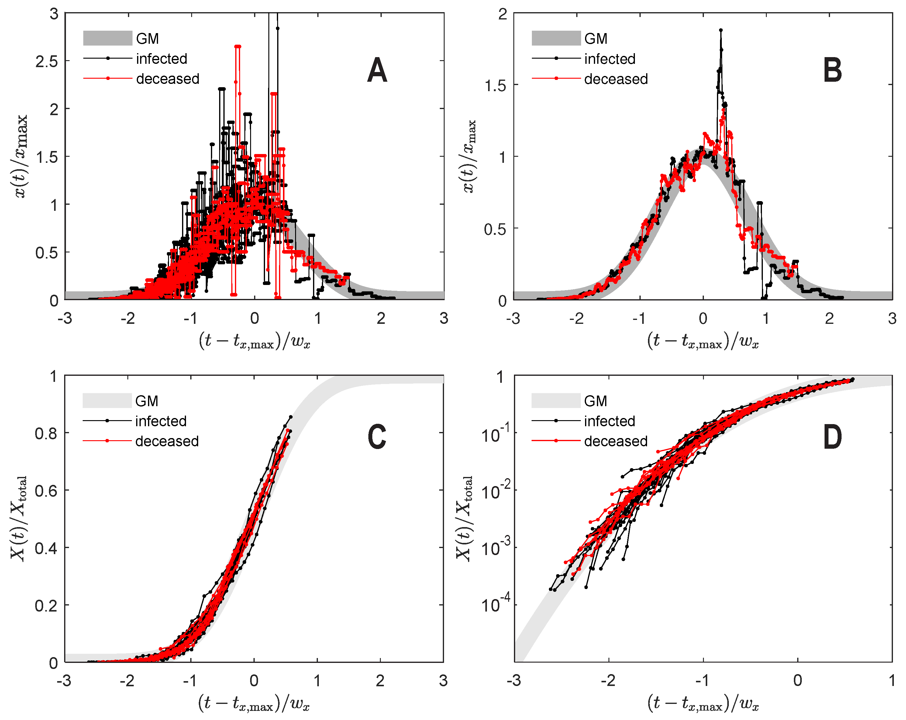
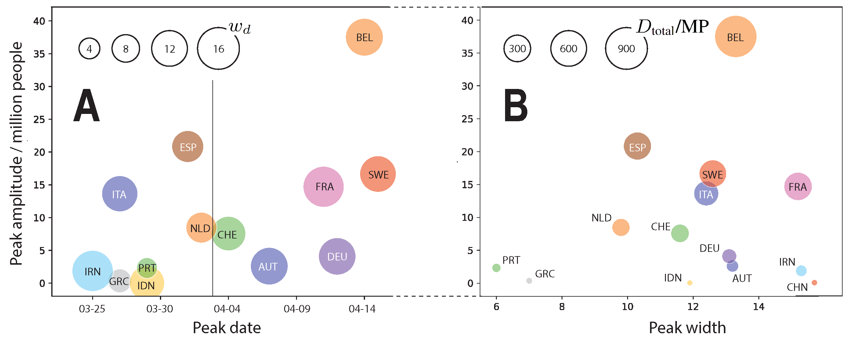
Using the fitted polynomial coefficients we compute the three parameters of the GM, i.e., maximum height, time of maximum height, and curve width, for each country. For mathematical details, please refer to the Appendix A. To demonstrate the universal Gaussian nature of the daily fatalities over time d, we display them in Figure 3A,B, normalized so that all curves have unit width, maximum, and time of maximum. The same plots for the cumulative fatalities D are shown in Figure 3C,D. Daily infections i, daily fatalities d, cumulative infections I and cumulative fatalities D, all fit neatly onto the unit GM curve or its cumulative function, plotted in gray in the back for reference. China, which is the only country to provide data from its first pandemic wave for times greater than (in normalized units), fits to the GM well over the entire significant course of infections and fatalities. This sparks the hope that the used GM will have predictive power for the remaining countries also after the maximum. The fits already provide sufficient evidence that the part prior to the maximum is captured well by the GM. The resulting GM parameters are listed and plotted in Table 1 and Figure 4. For most countries the GM width is within 10 and 15 days, roughly half of all countries have passed their peak of daily fatalities already and the peak is roughly below 20 fatalities per day and per million people.
2.4. Additional Predictions
Using the GM, one can obtain predictions for the further course of the Covid-19 pandemic analytically from the three descriptors. We here present two possible applications: cumulative fatalities as a function of time and the maximum required number of respiratory equipment as well as its time point.
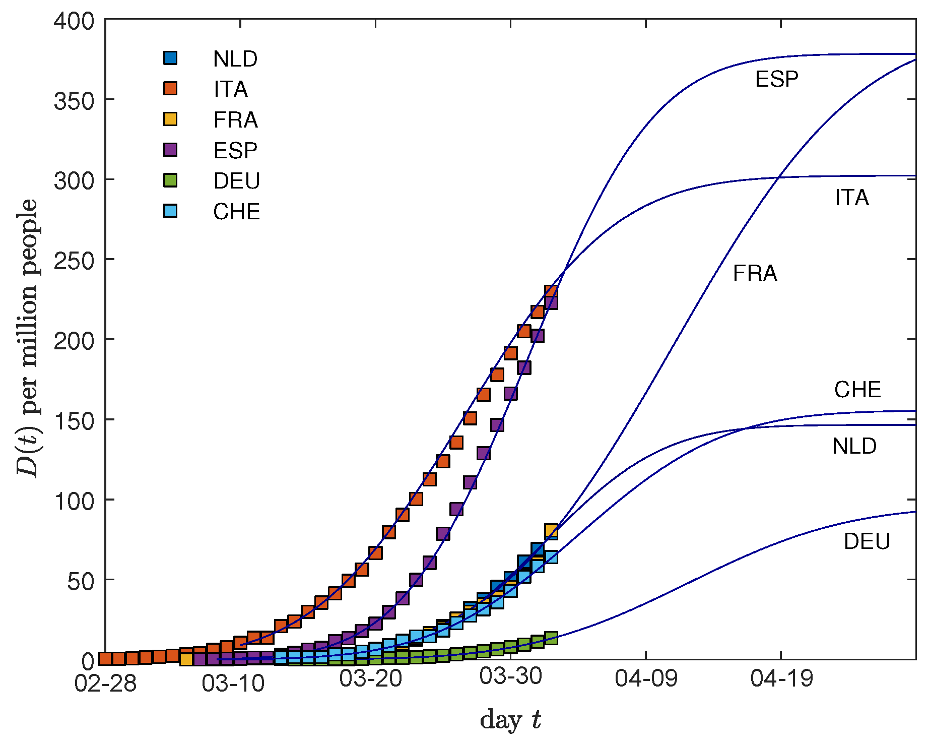
First, the time evolution of the number of cumulative fatalities D, plotted in Figure 5, can be obtained by summing daily number of deaths d, predicted by our model. In this figure, we rescaled all curves back to normal times so that the future course of cumulative deaths can be easily read-off. One can compute analytically that the date after which the new deaths per day have decreased to 1% of their maximum lies roughly 2 widths after the maximum of daily deaths, and the values, denoted by , for each country can be found in Table 1. Already from visual inspection Figure 5 suggests for Italy and Spain to plateau first, while France will have to face an increasing number of fatalities considerably longer. It also anticipates the cumulative number of fatalities per million people over the entire course of the Covid-19 disease to be highest for France, Spain, and Italy.
Next, we estimate the number of required respiratory machines per date for the Covid-19 epidemic. We start by assuming the number of respiratory machines per day to be equal to the cumulative number of active seriously sick persons on the given date, where active means not yet recovered by that date. Each new seriously sick person per day (SSP) requires a respiratory machine for some days or even weeks before passing away or recovering from Covid-19. According to other works [28], people who have died from Covid-19 occupied respiratory equipment for an average of 7 days prior to their death, but respiratory equipment may be in use for up to about one month for cases that later recovered. Thus, we may roughly estimate the number of active SSPs per date as the sum of people that became seriously sick within the past 10 days. Please note, however, that we try to only conceptually link the GM to useful quantities, we leave a thorough search of exact numbers to the reader.
As a final step, we need to relate SSPs and deaths. Assume that each SSP dies with a constant probability after some days, i.e., times SSPS gives the daily fatalities some days ahead. Taking again numbers from Ref. [28], we could use that each deceased patient had used a respiratory machine for an average of 7 days prior to death and thus estimate the daily number of SSPs at a given date by the number of daily fatalities 7 days in the future divided by probability .
The result of the above estimate reveals that the required number of respiratory equipment itself is a Gaussian curve, roughly centered around the same date as the daily fatality curve, and its peak value is proportional to a multiplicative factor that depends on the width of the Gaussianian and ranges between and for the widths we found, the total number of fatalities , and the ratio of passing away as a SSP .
3. Discussion
The preceding section demonstrated how a GM can be used to obtain statistical predictions for a pandemic such as the corona pandemic. The presentation was intentionally conceptual, to convey only the principle idea of such a model. It is clear that such predictions might work better for some countries than others. This is also why the reader should not be distracted too much by the large error in the fitted or derived parameters of Table 1.
The question remains, though, how the GM could be justified. In the following we aim to present a number of arguments in favor of the GM that make use of sigmoidal nature of the saturating processes such as pandemics and include a numerical argument on the stability of models.
First, let us list some other ’microscopic’ models that can lead to a Gaussian dynamics of fatalities or infections. One of the more prominent ones recently appeared in the Washington Post [30]. Stevens investigated what happens when simulitis spreads in a town, if everyone in the town starts at a random position, moving at a random angle, infecting others upon collision, and recovering after a certain time. The simulated number of infected people rises rapidly as the disease spreads and tapers off as people recover—a bell-shaped curve. We recreated the simulations and found evidence for the applicability of the GM under many circumstances. These results are not reported here, but support our central assumption. From another recent work using a holistic agent-based model [31], where the agents adapt their behavior through artificial intelligence as part of the solution, there seems also evidence from the numerical results presented, that the number of newly infected may be well captured by a Gaussianian. We went on and developed a new agent-based stochastic model described in detail in Appendix B, that can be seen as an efficient implementation of the situation explored in the Washington post. Our implementation does not require studying trajectories and collision events. Under most conditions this model results in a perfectly Gaussian-shaped daily number of fatalities.
The key of these behaviors lies in the sigmoidal nature of saturating processes. The derivative of sigmoidal functions have a bell-shaped form, similar to a Gaussian function, but may be asymmetric in general. We here model the daily fatalities d, formally the derivative of the cumulative fatalities D. Since we expect cumulative cases D to be sigmoidal, this fixes the derivative, the daily fatalities d, to a bell-shaped form. Even though all pandemics thus give rise to bell-shaped d by this argument, the curve’s parameters might differ, influenced mostly by policy, health system and culture. The predictive power of our model rests on the assumption that these influences are encoded already into the early data of casualties, combined with the assumption that a certain principal shape or a certain principal model of all pandemics is fixed.
Why do we choose a symmetric bell-shaped form, the Gaussian function? We recognize that other models, such as Poisson or gamma functions that fade out slower after their maximum, might be alternatively used. However, a symmetric function results from an agent-based model (Appendix B), it is the simplest model among all bell-shaped functions and works well enough to convey the idea of such models. Second, the times of greatest interest to policy makers are until the bell-curve’s peak since once passed the health system should be able to cope. Sigmoidal functions are popular to model saturation processes such as cellular growth [32,33] or enzyme (Michaelis–Menten) kinetics. Numerous sigmoidal functions exist and they have been used in many variations to predict infectious diseases [34] and have even been linked directly to models such as the SIR model [35]. Not surprisingly, sigmoidal models are frequently used in times of coronavirus [36,37,38], most often using a (generalized) logistic function (Richard’s curve). One model particularly similar to our GM [23] also uses the Gaussian integral as a sigmoidal function with similar parameters. However, the study only applies to the US, for which we noticed a bimodal Gaussian nature of d and thus decided not to model it here. Moreover, the precise methodology remains elusive as of today when we submitted this manuscript, but we assume the author fitted the sigmoidal Gaussian integral function, not its Gaussian derivative. We believe this to be a crucial difference to our procedure, to be discussed in the next paragraph.
A major issue with sigmoidal models is that they are often prone to overfitting [39] and also we in our preliminary experiments found such sigmoidal fits to be sensitive to initial conditions and to often require a large number of parameters. Previously, people have tried to experiment with regularizations [35] to account for such instabilities. Instead, we here choose to fit the logarithm of daily change of cases d, not the cumulative cases D. The logarithm of d weights more evenly values close to the function’s maximum and disregards other values. We believe this leads to a more reliable model of d around its maximum, the turning point of D, and the time of interest since most relevant predictions such as peak of the pandemic, time point, and width of peak are focused around this maximum.
The above arguments explained the necessity for sigmoidal models, but we also see mechanistic problems in other types of models, such as exponentials. Many exponential models rely on doubling times [24], which require intense preprocessing of data, such as smoothing, and are model dependent. Please refer to the methods in Appendix A for further discussion of doubling times in the context of the here presented GM. Other exponential models report considerable deviations from an exponential nature, e.g., a power law behavior as the curve flattens [40]. Sigmoidal functions automatically account for exponential growth and subsequent flattening.
We must note that we aim to be compared with descriptive models, i.e., models that work only in the statistical limit of large data. In contrast, mechanistic models for infectious diseases [27] are able to study the effect of parameters such as policies, health system, or culture on the outcome of a pandemic, and thus provide more detailed predictions and recommendations.
4. Conclusions
The here presented GM allows for simple predictions of future course of the Covid-19 disease and we have provided first evidence that a GM is able to capture the time evolution of the daily fatalities and infections per country. Fitted models describe past data well, including data from the first pandemic wave in China. As long as conditions such as the degree of social distancing remain unchanged, the GM is able to capture model data created by an agent-based approach, as we have demonstrated.
The model is so simple that it can be reproduced and applied without detailed knowledge of epidemiology, statistics, or programming languages. There are many countries not yet drastically affected by Covid-19, which will likely change for many in the coming weeks, and the GM could for example be used to apply it to such countries as soon as sufficient data is available. Using the recipe presented here, interested readers are in the position to obtain estimates for the shape of the Gaussian curve for their country, state, community, and use this model to compute more quantities of interest, such as our sketch of how to estimate the maximum number of required respiratory machines and the date of this maximum demand. Knowing the time of maximum rush days of SSPs, the maximum number of SSPs and width could help the government and medical agencies in these countries to optimize the management of the disease wave by appropriate drastic actions for limited time. Moreover, fortunately, as our study here demonstrates, the time of peak of the disease wave differs among countries. Knowledge of these peak times and their durations allows other countries to help those who undergo the peak of the wave at a significantly later time, with breathing apparati and trained medical personnel for a brief predictable time.
On one hand we are afraid our predictions will become reality, on the other they are more optimistic than all (few) predictions we came across so far. Confronting these predictions and the method with reality will help to either establish or rule out the presented approach. The applicability of the GM to describe the pandemic and its peak times for all countries, we will be able to judge in the far future. We are monitoring this development as part of our Supplementary Information.
5. Note Added in Proof
By the time this manuscript was under review several of the online available GM predictions could be used and also verified. The total number of fatalities in Germany after the first pandemic wave, accompanied by border openings, was 7897 on April 15 [25], while the GM predicted . As of today, three weeks later, this number increased to 8598 due to a daily number of deaths that presently remains at a relatively low and almost constant level of about . Similarly, as of today, June 3, the cumulated number of fatalities are 670 (Austria), 9522 (Belgium), 29024 (France), 179 (Greece), 1698 (Indonesia), 33601 (Italy), 8012 (Iran), 27128 (Spain), 1921 (Switzerland), 5996 (Netherlands), 1447 (Portugal), 4542 (Sweden), to be compared with Table 1. The only two countries for which we couldn’t make predictions on April 2, the United Kingdom and the United States (Table A1), as their coefficient of the GM had no sign within errors, turned out to suffer most from the pandemics, with 39811 and 107175 fatalities so far. A more detailed comparison is provided by our Supplementary website. The epidemological foundation of the GM will be a subject of our subsequent work.
Supplementary Materials
The following are available online at https://www.complexfluids.ethz.ch/corona, COVID-19 real time statistics and extrapolation using the Gauss model. This website provides parameters of the GM and GM predictions and allows to rate the performance of the GM model for more than 70 countries.
Author Contributions
R.S., F.S. initiated, M.K. and R.S. designed the study. M.K. developed the model, evaluated data, created figures. M.K. and R.S. prepared a draft. J.S. carefully restructured and extended the manuscript. All authors contributed to the final manuscript. All authors have read and agreed to the published version of the manuscript
Funding
This research received no external funding.
Acknowledgments
M.K. acknowledges major contributions by Clarisse Luap to the research and motivation of this work. She found, scanned and analyzed all available literature and sources of information related to Covid-19.
Conflicts of Interest
The authors declare no conflict of interest.
Appendix A. Model, Methods, and Implications of the GM
In this section we make the concepts used intuitively in the main text rigorous by introducing the necessary mathematical language.
Appendix A.1. Gauss Model
Denote the number of daily fatalities as a function of time by and the cumulative number of fatalities by , as in [24,41,42]. We model the time evolution of fatalities using the GM, i.e., a Gaussian function of time,
where denotes the width of the Gaussianian, denotes the maximum value of fatalities, and the time point at which this maximum is attained. The identical model and notation applies to the number of daily infections , cumulative infections and parameters , , .
We use publicly available data of monitored cumulative death rates , where the subscript m is used to distinguish data from our model, to derive the daily death rates by taking the first time derivative
and calculated its natural logarithm . The GM dynamics in Equation (A1) implies
which is a polynomial function of degree 2 with coefficients (note the minus sign in front of in Equation (A3))
The relevant parameters determining the number of deaths per day, the width of the distribution, as well as the position of the peak are then given by
Appendix A.2. Fitting and Errors
Using a second order polynomial fit to the data we obtained the coefficients , , as well as their confidence intervals. For this, the Matlab function [P,S,M]=polyfit(t,log(),2) on the natural logarithm of the monitored death rates yields the coefficients P=[,,] of the fit as well as information about the confidence intervals. We made use of the function polyparci that uses only core Matlab functions and does not require the Statistics Toolbox. It uses the procedures outlined in the polyfit documentation to calculate the covariance matrix, and uses functions betainc and fzero to calculate the cumulative t-distribution and the inverse t-distribution for a given probability and degrees-of-freedom. Within the limited amount of time we had to prepare this document, we were unable to compare error estimates from different approaches.
Appendix A.3. Deaths vs. Infections
We have applied the same procedure to the measured number of infected people, , giving rise to another set of parameters , , and . We found that the GM widths for infections and fatalities are similar in magnitude, within errors, and that and differ by a number of days [43], that can be considered constant for practical purposes. Our analysis confirms this estimate. It is also useful to introduce the fraction of fatalities among the truly infected (not the reported infected) , as this fraction can be expected to vary within limited bounds. We thus write
This reduces the number of parameters for a combined study of daily deaths and infections to four, as f cannot be considered constant, or further down to three, employing suggested by Figure 1 of Ref. [43]. We did not make use of these relationships and numbers anywhere in this work, but they can still be used to estimate quantities mentioned below. While this study mostly focuses on the number of fatalities, for reasons discussed, we had also included data from 11 countries for the reported number of infections in some of the previous figures that provide evidence for the applicability of the GM. Table A1 lists the corresponding parameters.

Table A1.
GM parameters , , and for those countries, for which sufficient data about infections, but insufficient data about fatalities is available to us, as of April 2. The coefficient we could not extract from the existing data with an error less than 100%. Parameters , , were used to create Figure 3.
| Code | Country | MP | ||||
|---|---|---|---|---|---|---|
| BRA | Brazil | 11.1 ± 0.2 | April 3 ± 8 | 800 ± 350 | 16,000 ± 7000 | 78 ± 35 |
| CHL | Chile | 11.7 ± 0.2 | April 2 ± 7 | 321 ± 33 | 6600 ± 800 | 370 ± 45 |
| GBR | Great Britain | 20.0 ± 0.7 | April 27 ± 14 | — | — | — |
| JPN | Japan | 38.0 ± 2.3 | April 27 ± 22 | 195 ± 90 | 13,000 ± 7000 | 104 ± 54 |
| SAU | Saudi Arabia | 15.4 ± 0.6 | April 2 ± 13 | 140 ± 23 | 3900 ± 700 | 120 ± 24 |
| SRB | Serbia | 10.3 ± 0.3 | April 1 ± 8 | 113 ± 50 | 2100 ± 1000 | 290 ± 130 |
| PAK | Pakistan | 10.3 ± 0.3 | March 28 ± 11 | 170 ± 80 | 3200 ± 1600 | 16 ± 8 |
| PER | Peru | 16.8 ± 1.3 | April 9 ± 28 | 148 ± 64 | 4400 ± 2300 | 140 ± 70 |
| POL | Poland | 15.0 ± 0.4 | April 7 ± 10 | 340 ± 50 | 9100 ± 1500 | 240 ± 40 |
| ROU | Romania | 18.9 ± 1.3 | April 19 ± 26 | 690 ± 90 | 23,200 ± 4600 | 1200 ± 250 |
| USA | United States | 14.8 ± 0.2 | April 14 ± 5 | — | — | — |
Appendix A.4. Data Used
Only countries which as of April 2 have reported more than 20 infected or 7 deceased people for more than 10 days. In addition, outliers that are better described by a multimodal extension of the GM have been omitted (including the United States) with the exception of China, for which there was a clear end of the first wave on about March 12. This resulted in the 25 countries used here. Using the identical approach, many more countries will be available for analysis within the next few days.
Appendix A.5. Cumulative Fatalities
The accumulated number of fatalities at time t, which we refer to as cumulative number of fatalities, is the integral of the daily fatalities in Equation (A1)
where is the projected total number of fatalities at and erf is the error function. Using Equation (A7), the time by which a first patient died from the virus is immediately estimated via . Similarly via for the first infected person, so-called patient 0, if one takes into account a time shift and ratio f between and , cf. Equation (A6), and one ignores the fact that the Gaussianian is likely to break down in this limit. The explicit expression is for the time of first appearance of Covid-19, and this time is specific for each country. Here, is the inverse error function. For values close to unity it is well approximated by .
Appendix A.6. Occupation of Respiratory Equipment
Most people that died from Covid-19 required respiratory equipment until their death for a period of length and we assumed this period to be constant. If people out of all that require respiratory equipment die, we can estimate the daily occupation of respiratory equipment by summing over the past days of newly seriously sick persons per day (SSPs), which are related to the daily deaths shifted by the typical time T from being diagnosed as seriously sick until death. For that, we divide the sum of deaths over the past days by to extrapolate to active SSPs at time t and hence required respiratory equipment
The number of required respiratory machines attains its maximum at time and thus the peak number of required respiratory machines is , where is the total number of deceased people. This peak increases with larger occupation times of respiratory machines , larger total number of fatalities and narrower GM widths . For the fitted values of and a of 10 days, the error function roughly is in the range . Flatten the curve!
Appendix A.7. Percentiles of Infection Numbers
From and we can estimate dates at which time the number of daily infected people i will have reduced to the level of of its maximum value. These times denoted as are given by
For and , these times are explicitly given, employing the typical delay time days, as seen in Equation (A6), by
The corresponding dates are listed for in Table 1. It is also possible to estimate dates, for which less than a certain of the total population remains infected and potentially dangerous to initiate another outbreak. This time is given by
where MP had been tabulated and visualized (Table 1, Figure 4), is the inverse error function, and f defined by Equation (A6) may be approximated by the value mentioned there. In this expression and can also be approximated by using the values calculated from fatalities, as described already. For (one per million inhabitants), and a typical , days for /MP .
Appendix A.8. Doubling Times
Doubling times, here denoted by k, are used to characterize the strength of an exponential growth process, independent of the exponential amplitude. A doubling time quantifies the time span required for the exponential to double (or, up to convention, to have doubled). Assuming a purely exponential growth, both and increase mono-exponentially with time, and the doubling time k is a constant, , while . For the GM the doubling time based on is thus given by
while the doubling time based on is given by . It is thus straightforward [44] to calculate two versions of doubling times with the GM parameters at hand, using either daily or total measures, which differ if the growth is not ideally exponential. While doubling times are convenient as they alter only weakly during exponential growth, they are difficult to extract from data directly without applying smoothing procedures that differ from publication to publication, and they are not uniquely defined. For this reason we do not recommend proceeding with an analysis on reported doubling times, as done in Ref. [24], unless the raw data is unavailable.
Appendix A.9. Reproduction Factor and Base Reproduction Number
The basic reproduction number of an infection can be thought of as the expected number of cases directly generated by one case in a population where all individuals are susceptible to infection [45,46]. The definition describes the state, in which no other individuals are infected or immunized (naturally or through vaccination). The basic reproduction number is not to be confused with the effective, time-dependent reproduction number , which is the number of cases generated in the current state of a population, which does not have to be the uninfected state. In Ref. [44], we provide both exact, and simple approximate relationships between the parameters of the GM and three variants of reproduction factors including basic reproduction numbers.
Appendix B. Stochastic Model Leading to Gaussian Time Evolution
To demonstrate that the so far somewhat unmotivated GM must not only be regarded as a minimal fit to a sigmoidal time-dependent evolution of daily cases, we here develop one of the possible models that incorporates selected aspects of a more ’microscopic’ or ’agent-based’ view of the dynamical evolution. The following is one of the type of models that seem to have some more rigorous foundation than the GM itself, and may thus provide advice if an underlying picture is required for a law that arises when large numbers of stochastic events lead to a seemingly deterministic outcome.
Consider the following probabilistic Monte Carlo algorithm to obtain the quadruplet (Table A2) for each person j at each time t, and calculate daily numbers for the whole population by summing over the individual contributions.
Table A2.
Let the current status of individual j among a population with P members at time t be characterized by a quadruplet with carrying for each individual four pieces of information as detailed in the table. While the identifiers , , carry binary information (1 = true, 0 = false) at time t, carries the time (a day number) at which person j got infected (, if this never happened). From these ’status’ quadruplets one can deduce, via the Monte Carlo algorithm described in the text part, quantities usually reported such as the daily number of fatalities. In addition, one has access to usually unknown true number of newly infected, currently infected, immune, never infected, deceased individuals, and their cumulative counterparts.
| person j | ||||
| status | infected | immune | dead | day of infection |
The model involves four parameters a, b, c, and f:
- a:
- duration in days, during which a newly infected person (not yet immune, or dead) can potentially infect others,
- b:
- average daily number of contacts between an infected person and other people randomly chosen from the whole population (dead or alive),
- c:
- probability for an infectious person to transmit the virus during a single contact (irrespective the health status of the contact, it might be healthy or already infected),
- f:
- probability to die from an infection.
We here treat them as constant, since this will eventually give rise to a Gaussian-shaped , but the model works without modification for any kind of time-dependent variation of the model parameters. The algorithm (verbally, followed by the code) involves the following steps:
- (0)
- Initialize.Code: Set time , , and for all .
- (1)
- Begin with a single infected individual (no 1) on day 0 of the pandemic.Code: , .
- (2)
- Proceed with the next day and clear the daily counters i (infected) and d (deceased) for later use.Code: Increase t by one. Set , , and .
- (3)
- Begin looping over all individuals at time t.Code:
- (4)
- If an individual j is infected, it dies today with probability .Code: If , choose an equally distributed random number . If , set , , ,
- (5)
- A deceased individual does not contribute to further infections.Code: If , proceed with step (3).
- (6)
- If an individual j is alive and already infected since more than a days, it gets immune today.Code: If and , then , .
- (7)
- If individual j is infected, inspect its contacts. If contact k is not yet immune, it is getting infected with probability c today.Code: If , create a set containing b people randomly chosen from the (dead or alive) population. For each member k of the set of contacts randomly choose a number : If and , then set , , .
- (8)
- Continue looping over all individuals.Code: If , proceed with step (3). Otherwise just continue with step (9),
- (9)
- Collect the daily information for later use.Code: Calculate current number of infected , immune , dead , and healthy people by summing over the information contained in the quadruplets. Note that cannot be derived from , while .
- (10)
- If there are no more infected people, terminate the code.Code: If , proceed with step (2), otherwise exit.
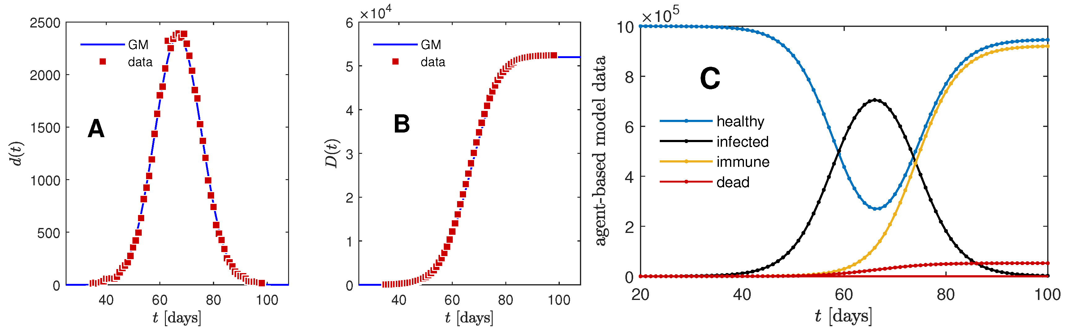
Upon completion, the total number of deaths is available, where is the daily number of deaths at time t. The total number of so far infected can be calculated via , where is the daily number of newly infected people. A typical simulation result is shown in Figure A1. The daily deaths , cumulative deaths , and also daily infections and cumulative infections are modeled well by the GM at a noise level that reduces with the population size (here ), and there is no hint that an asymmetry must be considered. This motivates the choice of a Gauss model to fit daily number of cases presented in this article. The relationship between the values of the four parameters a, b, c, f and the three parameters of the GM (width, time of peak, and peak value) within a region of applicability of the GM must remain beyond the scope of this manuscript.
Figure A1.
Representative result of our stochastic agent-based model. Model parameters: individuals, days, days, , and . There is no hint for an asymmetry to be taken into account and the GM describes the data for (A) daily fatalities and (B) cumulative fatalities very well. For this case the fitted GM parameters are , , and days. (C) Additional information available from the same simulation run, as described in the text part. Red data for cumulative fatalities is identical in (B,C).

References
- Kermack, W.O.; McKendrick, A.G. Contributions to the mathematical theory of epidemics—I. 1927. Bull. Mathem. Biol. 1991, 53, 33–55. [Google Scholar]
- Kermack, W.O.; McKendrick, A.G. Contributions to the mathematical theory of epidemics—II. The problem of endemicity. 1932. Bull. Mathem. Biol. 1991, 53, 57–87. [Google Scholar]
- Kermack, W.O.; McKendrick, A.G. Contributions to the mathematical theory of epidemics—III. Further studies of the problem of endemicity. 1933. Bull. Mathem. Biol. 1991, 53, 89–118. [Google Scholar]
- Enserink, M.; Kupferschmidt, K. With COVID-19, modeling takes on life and death importance. Science 2020, 367, 1414–1415. [Google Scholar] [CrossRef] [Green Version]
- Lixiang, L.; Yang, Z.; Dang, Z.; Meng, C.; Huang, J.; Meng, H.; Wang, D.; Chen, G.; Zhang, J.; Peng, H.; et al. Propagation analysis and prediction of the COVID-19. Infect. Dis. Model. 2020, 5, 282–292. [Google Scholar]
- Ciufolini, I.; Paolozzi, A. Mathematical prediction of the time evolution of the COVID-19 pandemic in Italy by a Gauss error function and Monte Carlo simulations. Eur. Phys. J. Plus 2020, 135, 355. [Google Scholar] [CrossRef] [PubMed]
- Pham, H. On estimating the number of deaths related to Covid-19. Mathematics 2020, 8, 655. [Google Scholar] [CrossRef]
- Cakir, Z.; Savas, H.B. A Mathematical Modelling Approach in the Spread of the Novel 2019 Coronavirus SARS-CoV-2 (COVID-19) Pandemic. Electr. J. Gen. Med. 2020, 17. [Google Scholar] [CrossRef] [Green Version]
- Alimadadi, A.; Aryal, S.; Manandhar, I.; Munroe, P.B.; Joe, B.; Cheng, X. Artificial intelligence and machine learning to fight COVID-19. Physiol. Genom. 2020, 52, 200–202. [Google Scholar] [CrossRef]
- Tarnok, A. Machine Learning, COVID-19 (2019-nCoV), and multi-OMICS. Cytometry A 2020, 97, 215–216. [Google Scholar] [CrossRef]
- Wynants, L.; Van Calster, B.; Bonten, M.M.J.; Collins, G.S.; Debray, T.P.A.; De Vos, M.; Haller, M.C.; Heinze, G.; Moons, K.G.M.; Riley, R.D.; et al. Prediction models for diagnosis and prognosis of covid-19 infection: Systematic review and critical appraisal. Brit. Medic. J. 2020, 369, m1328. [Google Scholar] [CrossRef] [Green Version]
- Singh, D.; Kumar, V.; Kaur, M. Classification of COVID-19 patients from chest CT images using multi-objective differential evolution-based convolutional neural networks. Europ. J. Clin. Microbiol. Infect. Dis. 2020. [Google Scholar] [CrossRef]
- Naude, W. Artificial intelligence vs COVID-19: Limitations, constraints and pitfalls. AI Soc. 2020. [Google Scholar] [CrossRef] [PubMed]
- Kim, S.; Seo, Y.B.; Jung, E. Prediction of COVID-19 transmission dynamics using a mathematical model considering behavior changes in Korea. Epidem. Health 2020, 42. [Google Scholar] [CrossRef]
- Zhu, Y.F.; Chen, Y.Q. On a Statistical Transmission Model in Analysis of the Early Phase of COVID-19 Outbreak. Statist. Biosci. 2020. [Google Scholar] [CrossRef]
- Bai, Z.H.; Gong, Y.; Tian, X.D.; Cao, Y.; Liu, W.J.; Li, J. The Rapid Assessment and Early Warning Models for COVID-19. Virol. Sin. 2020. [Google Scholar] [CrossRef] [PubMed] [Green Version]
- Wolfram, C. An agent-based model of Covid-19. Complex Syst. 2020, 29, 87–105. [Google Scholar] [CrossRef]
- National Center for Immunization and Respiratory Diseases (NCIRD). Covid-19 Forecasts. 2020. Available online: https://www.cdc.gov/coronavirus/2019-ncov/covid-data/forecasting-us.html (accessed on 2 April 2020).
- Sperrin, M.; Grant, S.W.; Peek, N. Prediction models for diagnosis and prognosis in Covid-19. Brit. Medic. J. 2020, 369. [Google Scholar] [CrossRef] [Green Version]
- Kristiansen, I.S.; Burger, E.A.; De Blasio, B.F. COVID-19: Simulation models for epidemics. Tidsskr. Nor. Laegeforening 2020, 140, 546–548. [Google Scholar]
- Panovska-Griffiths, J. Can mathematical modelling solve the current Covid-19 crisis? BMC Public Health 2020, 20. [Google Scholar] [CrossRef]
- Shrivastava, S.R.; Shrivastava, P. Resorting to mathematical modelling approach to contain the coronavirus disease 2019 (COVID-19) outbreak. J. Acute Dis. 2020, 9, 49–50. [Google Scholar] [CrossRef]
- Murray, C.J.L. Forecasting COVID-19 impact on hospital bed-days, ICU-days, ventilator-days and deaths by US state in the next 4 months. medRxiv 2020. [Google Scholar] [CrossRef] [Green Version]
- Schlickeiser, R.; Schlickeiser, F. A Gaussian model for the time development of the Sars-Cov-2 corona pandemic disease. Predictions for Germany made on March 30, 2020. Physics 2020, 2, 164–170. [Google Scholar] [CrossRef]
- Github databse. JSON Time-Series of Coronavirus Cases (Confirmed, Deaths and Recovered) Per Country-Updated Daily, 2020. Available online: https://pomber.github.io/covid19/timeseries.json (accessed on 2 April 2020).
- Barmparis, G.D.; Tsironis, G.P. Estimating the infection horizon of COVID-19 in eight countries with a data-driven approach. Chaos Solitons Fractals 2020, 135, 109842. [Google Scholar] [CrossRef]
- Adam, D. Special report: The simulations driving the world’s response to COVID-19. Nature 2020, 580, 316–318. [Google Scholar] [CrossRef] [Green Version]
- Yang, X.; Yu, Y.; Xu, J.; Shu, H.; Xia, J.; Liu, H.; Wu, Y.; Zhang, L.; Yu, Z.; Fang, M.; et al. Clinical course and outcomes of critically ill patients with SARS-CoV-2 pneumonia in Wuhan, China: A single-centered, retrospective, observational study. Lancet 2020, 8, 475–481. [Google Scholar] [CrossRef] [Green Version]
- Organisation for Economic Co-operation and Development (OECD). OECS Data. 2020. Available online: https://data.oecd.org (accessed on 3 April 2020).
- Stevens, H. Why Outbreaks Like Coronavirus Spread Exponentially, and How to Flatten the Curve. Washington Post. 2020. Available online: https://www.washingtonpost.com/graphics/2020/world/corona-simulator/ (accessed on 1 April 2020).
- Abhari, R.S.; Marini, M.; Chokani, N. COVID-19 epidemic in Switzerland: Growth prediction and containment strategy using artificial intelligence and big data. medRxiv 2020. [Google Scholar] [CrossRef] [Green Version]
- Zwietering, M.H.; Jongenburger, I.; Rombouts, F.M.; Van’t Riet, K. Modeling of the Bacterial Growth Curve. Appl. Environ. Microbiol. 1990, 56, 1875–1881. [Google Scholar] [CrossRef] [Green Version]
- Zullinger, E.M.; Ricklefs, R.E.; Redford, K.H.; Mace, G.M. Fitting Sigmoidal Equations to Mammalian Growth Curves. J. Mammal. 1984, 65, 607–636. [Google Scholar] [CrossRef]
- Hau, B. Mathematical Functions to Describe Disease Progress Curves of Double Sigmoid Pattern. Phytopathology 1993, 83, 928. [Google Scholar] [CrossRef]
- Wang, X.S.; Wu, J.; Yang, Y. Richards Model Revisited: Validation by and Application to Infection Dynamics. J. Theor. Biol. 2012, 313, 12–19. [Google Scholar] [CrossRef]
- Fu, X.; Ying, Q.; Zeng, T.; Wang, Y. Simulating and forecasting the cumulative confirmed cases of SARS-CoV-2 in China by Boltzmann function-based regression analyses. J. Infection 2020. [Google Scholar] [CrossRef] [PubMed]
- Wu, K.; Darcet, D.; Wang, Q.; Sornette, D. Generalized Logistic Growth Modeling of the COVID-19 Outbreak in 29 Provinces in China and in the Rest of the World. arXiv 2020, arXiv:2003.05681. [Google Scholar]
- Vasconcelos, G.L.; Macêdo, A.M.S.; Ospina, R.; Almeida, F.A.G.; Duarte-Filho, G.C.; Souza, I.C.L. Modelling Fatality Curves of COVID-19 and the Effectiveness of Intervention Strategies. medRxiv 2020. [Google Scholar] [CrossRef]
- Clark, F.; Brook, B.W.; Delean, S.; Reşit Akçakaya, H.; Bradshaw, C.J.A. The Theta-Logistic Is Unreliable for Modelling Most Census Data: Theta-Logistic Model Is Not Robust. Meth. Ecol. Evol. 2010. [Google Scholar] [CrossRef]
- Verma, M.K.; Asad, A.; Chatterjee, S. COVID-19 Epidemic: Power Law Spread and Flattening of the Curve. Trans Indian Natl. Acad. Eng. 2020. [Google Scholar] [CrossRef]
- Schüttler, J.; Schlickeiser, R.; Schlickeiser, F.; Kröger, M. Covid-19 predictions using a Gauss model, based on data from April 2. medRxiv 2020. [Google Scholar] [CrossRef] [Green Version]
- Schüttler, J.; Schlickeiser, R.; Schlickeiser, F.; Kröger, M. Covid-19 predictions using a Gauss model, based on data from April 2. Preprints 2020. [Google Scholar] [CrossRef] [Green Version]
- An der Heiden, M.; Buchholz, U. Modellierung von Beispielszenarien an der SARS-CoV-2 Epidemie 2020 in Deutschland. RKI 2020. (In Germany) [Google Scholar] [CrossRef]
- Kröger, M.; Schlickeiser, R. Gaussian doubling times and reproduction factors of the COVID-19 pandemic disease. Preprints 2020. [Google Scholar] [CrossRef]
- Milligan, G.N.; Barrett, A.D.T. Vaccinology: An Essential Guide; Wiley Blackwell: Chichester, UK, 2015; p. 310. [Google Scholar]
- Fraser, C.; Donnelly, C.A.; Cauchemez, S. Pandemic potential of a strain of influenza A (H1N1): Early findings. Science 2009, 324, 1557–1561. [Google Scholar] [CrossRef] [Green Version]
Figure 1.
(A) Gauss model (GM) for time evolution of a daily quantity (black) and the corresponding total quantity (red), which is the cumulative sum of until time t. (B) Consequences of varying the three parameters describing the GM: width , maximum height , and time of maximum height for both the daily (top) and total (bottom) rates. In this work, x stands for either deaths () or confirmed infections ().

Figure 2.
Logarithmic reported number of daily fatalities (squares) and the quadratic fits of number of daily fatalities (lines) over time for some countries. The plots demonstrate the quadratic nature of the logarithmic fatalities per day during times for which data already exists. The solid curves are GM predictions, according to Equation (A1). The fitted model (solid lines) can be used to extrapolate existing data to future times, to predict for example the time point of the maximum. This is what we use in the following to generate predictions based on the fit. The meaning of the GM parameters is highlighted in the inset. Raw data taken from Ref. [25]. These predictions as of April 2 are compared with latest data on our Supplementary website (https://www.complexfluids.ethz.ch/corona).

Figure 3.
Shifted and rescaled data separately for each of the 25 countries. (A) Number of daily infections and fatalities. (B) Obtained from data shown in (A) by averaging over entries at the same (bin size 0.01). (C) Number of cumulative infections and fatalities over time in normal scale, and (D) in logarithmic scale to appreciate different regimes with better resolution. Thick gray is the theory expression in Equation (A1) for daily, and Equation (A7) for cumulative casualties in (A–D). Data beyond are from China alone. Raw data taken from Ref. [25].

Figure 4.
(A) Plot of the fitted GM parameters , , and tabulated in Table 1. The horizontal lines mark the day of this study, April 2. China is missing in this plot as its occurred on February 17 according to our calculation. (B) Peak daily number of fatalities per 1 million inhabitants, i.e., divided by the number of inhabitants times .

Figure 5.
Measured cumulative number of deaths per one million inhabitants (symbols), compared with the GM predictions (A7) for selected fits of Table 1. The cumulative number of fatalities determining the height of the future plateau is given by the product of width and , times .

Table 1.
Fitted GM parameters , , and for those countries, for which sufficient data about fatalities is available by the time of writing. Error bars reported for 95% confidence intervals. The table lists the three fitted GM parameters (width, time of peak, and peak value), followed by estimated cumulative number of fatalities , per million people (MP), and the predicted dates from Equation (A10) at which the number of daily infected people had reduced to the level of of its maximum value. Number of inhabitants according to OECD [29]. For a plot of the fitted parameters see Figure 4. For China we considered only the data during the first pandemic wave, i.e., until a minimum in daily fatalities was reached on March 12.
| Code | Country | /MP | |||||
|---|---|---|---|---|---|---|---|
| AUT | Austria | 13.2 ± 1.5 | April 7 ± 21 | 21.6 ± 4.7 | 500 ± 170 | 60 ± 20 | April 25 ± 44 |
| BEL | Belgium | 13.3 ± 0.6 | April 14 ± 18 | 430 ± 26 | 10,200 ± 1100 | 890 ± 100 | May 3 ± 19 |
| CHE | Switzerland | 11.6 ± 0.5 | April 5 ± 17 | 63 ± 12 | 1300 ± 300 | 156 ± 37 | April 20 ± 1 |
| CHN | China | 15.7 ± 0.3 | February 17 ± 3 | 95 ± 3 | 2600 ± 100 | 1.9 ± 0.1 | March 11 ± 4 |
| DEU | Germany | 13.1 ± 0.4 | April 12 ± 10 | 340 ± 6 | 7900 ± 400 | 95 ± 5 | April 30 ± 11 |
| ESP | Spain | 10.3 ± 0.2 | April 1 ± 6 | 960 ± 70 | 17,500 ± 1600 | 380 ±35 | April 13 ± 7 |
| FRA | France | 15.2 ± 0.3 | April 11 ± 8 | 980 ± 320 | 26,000 ± 9000 | 390±140 | May 4 ± 9 |
| GRC | Greece | 7.0 ± 0.2 | March 27 ± 9 | 3.8 ± 1.3 | 47 ± 17 | 4.4 ± 1.6 | April 1 ± 7 |
| IDN | Indonesia | 11.9 ± 0.8 | March 19 ± 22 | 5.3 ± 4.7 | 111 ± 91 | 0.4 ± 0.4 | — |
| IRN | Iran | 15.3 ± 0.1 | March 25 ± 2 | 150 ± 14 | 4100 ± 400 | 51 ± 5 | April 17 ± 2 |
| ITA | Italy | 12.4 ± 0.1 | March 27 ± 1.8 | 832 ± 60 | 18,300 ± 1400 | 300 ± 23 | April 12 ± 2 |
| NLD | Netherlands | 9.8 ± 0.1 | April 2 ± 4 | 144 ± 23 | 2500 ± 400 | 147 ± 26 | April 13 ± 5 |
| PRT | Portugal | 6.0 ± 0.1 | March 29 ± 4 | 24 ± 4 | 260 ± 40 | 25 ± 4 | April 2 ± 4 |
| SWE | Sweden | 12.6 ± 1.2 | April 15 ± 35 | 162 ± 12 | 3600 ± 600 | 370 ± 60 | May 1 ± 35 |
© 2020 by the authors. Licensee MDPI, Basel, Switzerland. This article is an open access article distributed under the terms and conditions of the Creative Commons Attribution (CC BY) license (http://creativecommons.org/licenses/by/4.0/).
Share and Cite
MDPI and ACS Style
Schüttler, J.; Schlickeiser, R.; Schlickeiser, F.; Kröger, M. Covid-19 Predictions Using a Gauss Model, Based on Data from April 2. Physics 2020, 2, 197-212. https://0-doi-org.brum.beds.ac.uk/10.3390/physics2020013
AMA Style
Schüttler J, Schlickeiser R, Schlickeiser F, Kröger M. Covid-19 Predictions Using a Gauss Model, Based on Data from April 2. Physics. 2020; 2(2):197-212. https://0-doi-org.brum.beds.ac.uk/10.3390/physics2020013
Chicago/Turabian StyleSchüttler, Janik, Reinhard Schlickeiser, Frank Schlickeiser, and Martin Kröger. 2020. "Covid-19 Predictions Using a Gauss Model, Based on Data from April 2" Physics 2, no. 2: 197-212. https://0-doi-org.brum.beds.ac.uk/10.3390/physics2020013