Kinetic Freeze-Out Properties from Transverse Momentum Spectra of Pions in High Energy Proton-Proton Collisions


Institute of Theoretical Physics & State Key Laboratory of Quantum Optics and Quantum Optics Devices, Shanxi University, Taiyuan 030006, China
*
Author to whom correspondence should be addressed.
Physics 2020, 2(2), 277-308; https://0-doi-org.brum.beds.ac.uk/10.3390/physics2020015
Submission received: 21 May 2020
/
Revised: 8 June 2020
/
Accepted: 9 June 2020
/
Published: 12 June 2020
(This article belongs to the Special Issue Statistical Approaches in High Energy Physics)
Abstract
:Transverse momentum spectra of negative and positive pions produced at mid-(pseudo)rapidity in inelastic or non-single-diffractive proton-proton collisions over a center-of-mass energy, , range from a few GeV to above 10 TeV are analyzed by the blast-wave fit with Boltzmann (Tsallis) distribution. The blast-wave fit results are well fitting to the experimental data measured by several collaborations. In a particular superposition with Hagedorn function, both the excitation functions of kinetic freeze-out temperature () of emission source and transverse flow velocity () of produced particles obtained from a given selection in the blast-wave fit with Boltzmann distribution have a hill at GeV, a drop at dozens of GeV, and then an increase from dozens of GeV to above 10 TeV. However, both the excitation functions of and obtained in the blast-wave fit with Tsallis distribution do not show such a complex structure, but a very low hill. In another selection for the parameters or in the superposition with the usual step function, and increase generally quickly from a few GeV to about 10 GeV and then slightly at above 10 GeV, there is no such the complex structure, when also studying nucleus-nucleus collisions.
Keywords:
excitation function of kinetic freeze-out temperature; excitation function of transverse flow velocity; proton–proton collisionsPACS:
14.40.Aq; 13.85.Hd; 13.75.Cs1. Introduction
Chemical and thermal or kinetic freeze-outs are two of important stages of system evolution in high energy collisions. The excitation degrees of interacting system at the two stages are possibly different from each other. To describe different excitation degrees of interacting system at the two stages, one can use chemical and kinetic freeze-out temperatures respectively. Generally, at the stage of chemical freeze-out, the ratios of different types of particles are no longer changed, and the chemical freeze-out temperature can be obtained from the ratios of different particles in the framework of thermal model [1,2,3]. At the stage of kinetic freeze-out, the transverse momentum spectra of different particles are no longer changed, and the dissociation temperature [4] or kinetic freeze-out temperature can be obtained from the transverse momentum spectra according to the hydrodynamical model [4] and the subsequent blast-wave fit with Boltzmann distribution [5,6,7] or with Tsallis distribution [8,9,10].
It should be pointed out that the transverse momentum spectra even though in narrow range contain both the contributions of random thermal motion and transverse flow of particles. The random thermal motion and transverse flow reflect the excitation and expansion degrees of the interacting system (or emission source) respectively. To extract the kinetic freeze-out temperature from transverse momentum spectra, we have to exclude the contribution of transverse flow, that is, we have to disengage the random thermal motion and transverse flow. There are more than one methods to disengage the two issues [4]. The simplest and easiest method is to use the blast-wave fit with Boltzmann distribution [5,6,7] and with Tsallis distribution [8,9,10] to analyze the transverse momentum spectra, though other method such as the alternative method [6,11,12,13,14,15,16,17] can obtain similar results [18].
The early blast-wave fit is based on the Boltzmann distribution [5,6,7]. An alternative blast-wave fit is used due to the Tsallis distribution [8,9,10]. Both types of blast-wave fit can be used to disengage the random thermal motion and transverse flow. Then, the kinetic freeze-out temperature of interacting system and transverse flow velocity of light flavor particles can be extracted. Most of light flavor particles are produced in soft excitation process and have narrow transverse momentum range up to 2∼3 GeV/c. A few part of light flavor particles are produced in hard scattering process and have higher transverse momenta. Generally, heavy flavor particles are produced via hard scattering process. From the point of view of disengaging or extraction, particles produced in hard scattering process are not needed to consider by us.
The excitation function of kinetic freeze-out temperature, that is, the dependence of kinetic freeze-out temperature on collision energy, is very interesting for us to study the properties of high energy collisions. We think that the particular change of excitation functions of kinetic freeze-out temperature and other parameters are related to the critical-end-point (CEP) of phase transition from hadronic matter to quark-gluon plasma (QGP or quark matter) happened in central nucleus-nucleus ( or A-A) collisions, where the particular change means the appearances of saturation, minimum, maximum, knee point, asymptotical line, etc. For high multiplicity proton–proton ( or p-p) collisions, even for minimum-bias collisions, the particular change of excitation functions of some parameters are expected to compare with those in collisions, where the quark degree of freedom in minimum-bias collisions is expected to play initially a main role at the energy of particular change, though QGP is not expected to form in minimum-bias collisions due to small system and products. The minimum of excitation function is also related to the soft point of equation of state (EOS) of hadronic matter or QGP, which is also related to the phase transition.
Although there are many studies on the excitation functions of kinetic freeze-out temperature and other parameters, the results seem to be inconsistent. For example, over a center-of-mass energy per nucleon pair, , range from a few GeV to a few TeV, the excitation function of kinetic freeze-out temperature in gold-gold (Au-Au) and lead-lead (Pb-Pb) collisions initially increases and then inconsistently saturates [19,20], increases [21], or decreases [22,23] with the increase of collision energy. On the contrary, the excitation function of the chemical freeze-out temperature shows initially increases and then consistently saturates with collision energy [1,2,3,4]. Comparatively, as the basic processes in collisions, collisions are very important in the study of the mentioned excitation functions. However, the excitation functions in collisions are short of studies. We hope to study the particular changes of excitation functions in collisions due to they being also related to quark degree of freedom, but not QGP. Indeed, it is worth to study the excitation functions of kinetic freeze-out temperature and other parameters in collisions and to judge their tendencies over an energy range from GeV to TeV.
In this paper, by using the blast-wave fit with Boltzmann distribution [5,6,7] and with Tsallis distribution [8,9,10], we study the excitation functions of some concerned quantities in inelastic (INEL) or non-single-diffractive (NSD) collisions which are closer to peripheral nuclear collisions comparing with central ones. The experimental transverse momentum spectra of negative and positive pions ( and ) measured mainly at the mid-rapidity by the NA61/SHINE Collaboration [24] at the the Super Proton Synchrotron (SPS) and its beam energy scan (BES) program, the PHENIX [25] and STAR [6] Collaborations at the Relativistic Heavy Ion Collider (RHIC), as well as the ALICE [26] and CMS [27,28] Collaborations at the Large Hadron Collider (LHC) are analyzed, while the data in the forward and backward rapidity regions are not available in most cases.
The remainder of this paper is structured as follows. The formalism and method are shortly described in Section 2. Results and discussion are given in Section 3. In Section 3.1, we summarize our main observations and conclusions.
2. Formalism and Method
There are two main processes of particle productions, namely the soft excitation process and the hard scattering process, in high energy collisions. For the soft excitation process, the method used in the present work is the blast-wave fit [5,6,7,8,9,10] that has wide applications in particle productions. The blast-wave fit is based on two types of distributions. One is the Boltzmann distribution [5,6,7] and another one is the Tsallis distribution [8,9,10]. As an application of the blast-wave fit, we present directly its formalisms in the following. Although the blast-wave fit has abundant connotations, we focus only our attention on the formalism of transverse momentum () distribution in which the kinetic freeze-out temperature () and mean transverse flow velocity () are included.
We are interested in the blast-wave fit with Boltzmann distribution in its original form. According to [5,6,7], the blast-wave fit with Boltzmann distribution results in the probability density distribution of to be
where is the normalized constant, is the transverse mass, is the rest mass, r is the radial coordinate in the thermal source, R is the maximum r which can be regarded as the transverse size of source in the case of neglecting the expansion, is the relative radial position which has in fact more meanings than r and R themselves, and are the modified Bessel functions of the first and second kinds respectively, is the boost angle, is a self-similar flow profile, is the flow velocity on the surface, and is used in the original form [5]. There is the relation between and . As a mean of , .
We are also interested in the blast-wave fit with Tsallis distribution in its original form. According to [8,9,10], the blast-wave fit with Tsallis distribution results in the distribution to be
where is the normalized constant, q is an entropy index that characterizes the degree of non-equilibrium, denotes the azimuthal angle, and is used in the original form [8]. Because of being an insensitive quantity, the results corresponding to and 2 for the blast-wave fit with Boltzmann or Tsallis distribution are harmonious [18]. In fact, in some literature [29], is regarded as a free parameter which changes largely by several times and increases 1 in the number of free parameter, which is not our expectation in the present work. In addition, the index used in Equation (2) can be replaced by due to q being very close to 1. This substitution results in a small and negligible difference in the Tsallis distribution [30,31].
For a not too wide spectrum, the above two equations can be used to describe the spectrum and to extract and . For a wide spectrum, we have to consider the contribution of hard scattering process. According to the quantum chromodynamics (QCD) calculus [32,33,34], the contribution of hard scattering process is parameterized to be an inverse power-law
which is the Hagedorn function [35,36], where and n are free parameters, and A is the normalization constant related to the free parameters. In literature [37,38,39,40,41,42,43], there are respectively modified Hagedorn functions
and
where the three normalization constants A, free parameters , and free parameters n are severally different, though the same symbols are used to avoid trivial expression.
The experimental spectrum distributed in a wide range can be described by a superposition of the contributions of the soft excitation and hard scattering processes. If one of Equations (1) and (2) describes the contribution of the soft excitation process, one of Equations (3)–(6) describes the contribution of the hard scattering process. To describe the spectrum in a wide range, we can superpose a two-component superposition like this
where k () denotes the contribution fraction of the soft excitation (hard scattering) process, and denotes one of Equations (1) and (2). As for the four , we are inclined to the first one due to its more applications. Naturally, we have the normalization condition , where denotes the maximum . In Equation (7), the soft component contributes in low region and the hard component contributes in whole range. The two contributions overlap each other in low region.
According to Hagedorn’s model [35], we may also use the usual step function to superpose the two functions. That is
where and are constants which result in the two components to be equal to each other at GeV/c. The contribution fraction of the soft excitation (hard excitation) process in Equation (8) is [] due to . In Equation (8), the soft component contributes in low region and the hard component contributes in high region. The two contributions link with each other at .
In some cases, the contribution of resonance production for pions in very-low range has to be considered. We can use a very-soft component for the range from 0 to 0.2∼0.3 GeV/c which covers the contribution of resonance production. Let and denote the contribution fractions of the very-soft and soft processes respectively. Equation (7) is revised to
where denotes one of Equations (1) and (2) as , but having smaller parameter values comparing with . Anyhow, both the very-soft and soft processes are belong to the soft process. Correspondingly, Equation (8) is revised to
where , , and are constants which result in the two contiguous components to be equal to each other at and .
The above two types of superpositions [Equations (7) and (8)] treat the soft and hard components by different ways in the whole range. Equation (7) means that the soft component contributes in a range from 0 up to 2∼3 GeV/c or a little more. The hard component contributes in the whole range, though the main contributor in the low region is the soft component and the sole contributor in the high region is the hard component. Equation (8) shows that the soft component contributes in a range from 0 up to , and the hard component contributes in a range from up to the maximum. The boundary of the contributions of soft and hard components is . There is no mixed region for the two components in Equation (8).
In the case of including only the soft component, Equations (7) and (8) are the same. In the case of including both the soft and hard components, their common parameters such as , , , and n should be severally to have small differences from each other. To avoid large differences, we should select the experimental data in a narrow range. In addition, the very-soft component in Equations (9) and (10) does not need to consider in some cases due to the fact that the spectrum in very-low range are possibly not available in experiment. Then, Equations (9) and (10) are degenerated to Equations (7) and (8) respectively in some cases.
In the fit process, firstly, we use Equation (7) to extract the related parameters, where and are exactly Equations (1) or (2) and (3) respectively. Regardless of Equation (1) or (2) is regarded as , the situation is similar due to Equations (1) and (2) being harmonious in trends of parameters [18], though one more parameter (the entropy index q) is needed in Equation (2). Secondly, we use Equation (8) to extract the related parameters as comparisons with those from Equations (7). In the case of Equations (7) and (8) being not suitable, Equations (9) and (10) can be used due to the very-low component from resonance decays being included in the first items of the two fits. Meanwhile, the contribution of resonance decays in the low component is naturally included in the second items of Equations (9) and (10) or in the first items of Equations (7) and (8). Thus, the contribution of resonance decays which is available in the very-low or low component in experiment is naturally considered by us.
It should be pointed out that although Equations (9) and (10) are not used in the final fits in the present work, we hope to keep them here due to the fact that we need them to give further explanations. From theses explanations, one can see the relations between Equations (9)/(10) and (7)/(8), as well as possible applications of Equations (9) and (10).
3. Results and Discussion
3.1. Comparison with Data by Equation (7)
Figure 1 shows the transverse momentum spectra of and produced at mid-(pseudo)rapidity in collisions at high center-of-mass energies, where different mid-(pseudo)rapidity (y or ) intervals and energies () are marked in the panels. Different forms of the spectra are used due to different Collaborations, where N, E, p, , and denote the particle number, energy, momentum, cross-section, and event number, respectively. The closed and open symbols presented in panels (a)–(e) represent the data of and measured by the NA61/SHINE [24], PHENIX [25], STAR [6], ALICE [26], and CMS [27,28] Collaborations, respectively, where in panel (a) only the spectra of are available, and panel (c) is for NSD events and other panels are for INEL events. Although the collisions are divided on the multiplicity classes in experiments on the LHC, we have used the minimum-bias INEL events [26,27,28] which can be regarded as the combination of the events in different multiplicity classes with different yields. We regret not using the ATLAS Collaboration results [44,45,46,47,48] given no data on the spectra of and . These data show wider spectra of charged particles to be used in our foreseen studies. In some cases, different amounts marked in the panels are used to scale the data for clarity. We have fitted the data by two sets of parameter values in Equation (7) so that we can see the fluctuations of parameter values. The blue solid (dotted) curves are our results for () spectra fitted by Equation (7) through Equations (1) and (3), and the blue dashed (dot-dashed) curves are our results for () spectra fitted by Equation (7) through Equations (2) and (3), by the first set of parameter values, in which k is taken to close to 0.5 as much as possible. The black curves are our results fitted by the second set of parameter values for comparison, in which k is taken to close to 1 as much as possible. The values of free parameters (, , q if available, k, , and n), normalization constant (), , and number of degrees of freedom (ndof) corresponding to the curves in Figure 1 are listed in Table 1 and Table 2, where the errors of fit parameters are obtained by the statistical simulation method [49], no matter what /ndof is. The parameter values presented in terms of value/value denote respectively the first and second sets of parameter values in Equation (7) through Equations (1)–(3) in which . One can see that Equation (7) with two sets of parameter values describes the spectra at mid-(pseudo)rapidity in collisions over an energy range from a few GeV to above 10 TeV. The blast-wave fit with Boltzmann distribution and with Tsallis distribution presents similar results. The free parameters show some laws in the considered energy range. For a given parameter, its fluctuation at given energy is obvious in some cases. Because of the data being not available in very-low range, Equation (9) is not used in the fit.
It should be noted that, from the fit process we know that, the Tsallis expression, Equation (2), having a polynomial behavior at large could be a better description for the spectra at large values of , where the Boltzmann expression, Equation (1) does not work possibly at large if we use the same parameters and . In some cases, for the spectra in a wide range, a single Tsallis expression is suitable, and two- or three-component Boltzmann expression is needed. Our previous work [50] studied both the Tsallis and Boltzmann distributions without flow effect and also confirms this issue. Indeed, the Tsallis description is better than the Boltzmann one, though the former has one more parameter q. In fact, the introduction of the entropy index q in the Tsallis description has the meaning of reality. As discussed in Section 2, q characterizes the degree of non-equilibrium. In addition, when , the Tsallis description degenerates to the Boltzmann one.
To see clearly the excitation functions of free parameters, Figure 2a–e show the dependences of , , , n, and k on , respectively. The blue and black closed and open symbols represent the parameter values corresponding to and respectively, which are listed in Table 1 and Table 2. The blue circles (black squares) represent the first set of parameter values obtained from Equation (7) through Equations (1)–(3). The blue asterisks (black triangles) represent the second set of parameter values obtained from Equation (7) through Equations (1)–(3). One can see that the difference between the results of and is not obvious. In the excitation functions of the first set of and obtained from the blast-wave fit with Boltzmann distribution, there are a hill at GeV, a drop at dozens of GeV, and then an increase from dozens of GeV to above 10 TeV. In the excitation functions of the first set of and obtained from the blast-wave fit with Tsallis distribution, there is no the complex structure, but a very low hill. In the excitation functions of the second set of and , there is a slight increase from about 10 GeV to above 10 TeV. In Equation (7) contained the blast-wave fit with both distributions, in the excitation functions of and n, there are a slight decrease and increase respectively in the case of the hard component being available. The excitation function of k shows that the contribution () of hard component slightly increases from dozens of GeV to above 10 TeV, and it has no contribution at around 10 GeV. At given energies, the fluctuations in a given parameter result in different excitation functions due to different selections. As a comparison, the red asterisks (green triangles) in Figure 2 represent the results from collisions which are discussed in detail in the Appendix A. One can see that the results from collisions approach to those from collisions with the second set of parameters, though only the soft component is used in most cases.
Indeed, GeV is a special energy for collisions as indicated by Cleymans [51]. The present work shows that GeV is also a special energy for collisions. In particular, there is a hill in the excitation functions of and in collisions due to a given selection of the parameters. At this energy (11 GeV more specifically [51]), the final state has the highest net baryon density, a transition from a baryon-dominated to a meson-dominated final state takes place, and the ratios of strange particles to mesons show clear and pronounced maximums [51]. These properties result in this special energy.
At 11 GeV, the chemical freeze-out temperature in collisions is about 151 MeV [51], and the present work shows that the kinetic freeze-out temperature in collisions is about 105 MeV, extracted from the blast-wave fit with Boltzmann distribution. If we do not consider the difference between and collisions, though cold nuclear effect exists in collisions, the chemical freeze-out happens obviously earlier than the kinetic one. According to an ideal fluid consideration, the time evolution of temperature follows , where (=300 MeV) and (=1 fm) are the initial temperature and proper time respectively [52,53], and and denote the final temperature and time respectively, the chemical and kinetic freeze-outs happen at 7.8 and 23.3 fm respectively. It should be noted that in the calculation of , the Lorentz factor is not considered. If we consider the mean Lorentz factor (–6) of charged pions in the rest frame of emission source [15,16,17,18], the value of freeze-out time will be smaller.
Strictly, () obtained from the pion spectra in the present work is less than that averaged by weighting the yields of pions, kaons, protons, and other light particles. Fortunately, the fraction of the pion yield in high energy collisions are major (≈85%). The parameters and their tendencies obtained from the pion spectra are similar to those obtained from the spectra of all light particles. To study the excitation functions of and , it does not matter if we use the spectra of pions instead of all light particles.
It should be noted that the main parameters and are correlated in some way. Although the excitation functions of () which are acceptable in the fit process are not sole, their tendencies are harmonious in most cases, in particular in the energy range from the RHIC to LHC. Combining with our previous work [18], we could say that there is a slight (≈10%) increase in the excitation function of and an obvious (≈35%) increase in the excitation function of from the RHIC to LHC. At least, the excitation functions of and do not decrease from the RHIC to LHC.
However, the excitation function of from low to high energies is not always incremental or invariant, though the excitation function of has the trend of increase in general. For example, In [4], slowly decreases as increases from 23 GeV to 1.8 TeV, and slowly increases with . In [19,20], has no obvious change and has a slight (≈10%) increase from the RHIC to LHC. In [21], has a slight (≈9%) increase and has a large (≈65%) increase from the RHIC to LHC. In [22,23], has a slight (≈5%) decrease from the RHIC to LHC and increases by ≈20% from 39 to 200 GeV. It is convinced that increases from the RHIC to LHC, though the situation of is doubtful.
Although some works [54,55,56,57] reported a decrease of and an increase of from the RHIC to LHC, our re-scans on their plots show a different situation of . For example, in [54], our re-scans show that has no obvious change and has a slight (≈9%) increase from the top RHIC to LHC, though there is an obvious hill or there is an increase by ≈30% in in 5–40 GeV comparting with that at the RHIC. Authors in [55] shows similar results to [54] with the almost invariant from the top RHIC to LHC, an increase by ≈28% in in 7–40 GeV comparing with that at the top RHIC, and an increase by ≈8% in comparing with that at the top RHIC. Authors in [56,57] shows similar result to [54,55] on , though the excitation function of is not available.
In some cases, the correlation between and are not negative, though some works [54,55] show negative correlation over a wide energy range. For a give spectrum, it seems that a larger corresponds to a smaller , which shows a negative correlation. However, this negative correlation is not sole case. In fact, a couple of suitable and can fit a given spectrum. A series of spectra at different energies possibly show a positive correlation between and , or independent of on , in a narrow energy range. Very recently, authors in [58] shows approximately independent of on in collisions at TeV, and negative correlations in p-Pb collisions at TeV and in Pb-Pb collisions at TeV, for different average charged-particle multiplicity densities, i.e., for different centrality classes. These results are partly in agreement with our results. It seems that the correlation between and is an open question at present, though some researchers think that there is a negative correlation between and . In our opinion, the type of correlation between and depends on three factors, that is the choices of fitted region in low and medium range, fixed or changeable , sensitivity of on centrality. Indeed, more studies are needed in the near future.
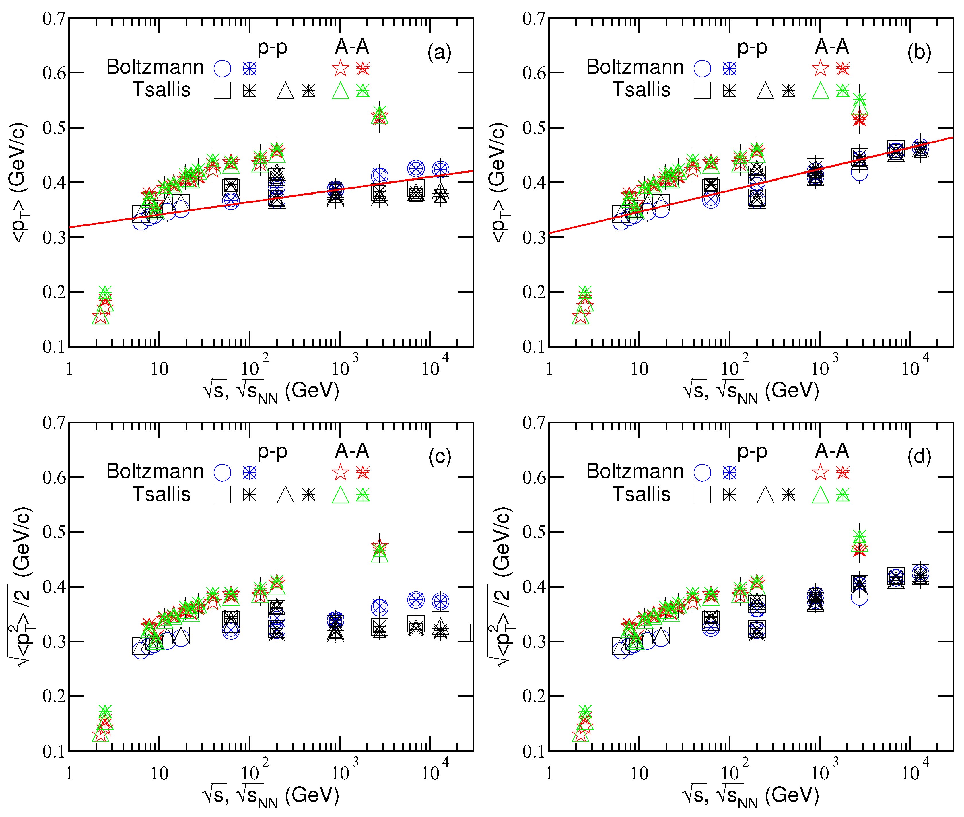
To study further the behaviors of parameters, Figure 3 shows the excitation functions of (a)(b) mean () and (c)(d) ratio of root-mean-square () to , where the left panel [(a)(c)] corresponds to the results of the first component [Equation (1) or (2)] and the right panel [(b)(d)] corresponds to the results of the two components [Equation (7)]. The open symbols (open symbols with asterisks) represent the values corresponding to () spectra. The blue circles (black squares) represent the values obtained indirectly from Equations (1) and (2) for the left panel or Equation (7) through Equations (1)–(3) for the right panel, by the first set of parameter values. The results by the second set of parameter values are presented by the blue asterisks (black triangles). These values are indirectly obtained from the equations according to the parameters listed in Table 1 and Table 2 over a range from 0 to 5 GeV/c which is beyond the available range of the data. If the initial temperature of interacting system is approximately presented by [59,60,61], the lower panel shows the excitation function of initial temperature. Because of excluding different contribution fractions of the second component, the left panel [(a)(c)] shows some differences in the case of using two sets of parameter values. It should be noted that the root-mean square momentum component of particles in the rest frame of isotropic emission source is regarded as the initial temperature, or at the least it is a reflection of the initial temperature. The relations in the left panel are complex and multiple due to different sets of parameter values. The line in Figure 3b is fitted to various symbols by linear function
with /ndof = 54/82. From the line one can see that the behavior of . In particular, with the increase of and including the contribution of second component, increases approximately linearly. As a comparison, the red asterisks (green triangles) in Figure 3 represent the results for collisions, which are indirectly obtained according to the parameter values listed in Table A1 and Table A2. One can see that the results for collisions are greater than those for collisions at around 10 GeV and above.
The quantities and are very important to understand the excitation degree of interacting system. As for the right panel in Figure 3 which is for the two-component, the incremental trend for and with the increase of () is a natural result due to more energy deposition at higher energy. Although and are obtained from the parameter values listed in Table 1 and Table 2 (A1 and A2), they are independent of fits or models. More investigations on the excitation functions of and are needed due to their importance.
3.2. Comparison with Data by Equation (8)
To discuss further, for comparisons with the results from Equation (7), we reanalyze the spectra by Equation (8) and study the trends of new parameters. Figure 4 is the same as Figure 1, but showing the results fitted by Equation (8) through Equations (1) and (3) and through Equations (2) and (3) respectively. For Equation (8) through Equations (1) and (3), only one set of parameter values are used due to the fact that there is no correlation in the extraction of parameters in the two-component fit. For Equation (8) through Equations (2) and (3), two sets of parameter values are used to see the insensitivity of main parameters. The first set of parameter values are obtained by the method of least squares. The second set of parameter values are obtained by increasing or decreasing main parameters (, , q, and k) by a few percent, and limits the increase of by a few percent. The values of related parameters are listed in Table 3 and Table 4 which are the same as Table 1 and Table 2 respectively, and with only one set of parameter values in Table 3. The related parameters are shown in Figure 5 and the leading-out parameters are shown in Figure 6, which are the same as Figure 2 and Figure 3 respectively, and with only one set of parameter values for Equation (8) through Equations (1) and (3). In particular, k in Figure 5 is obtained by due to is normalized to 1, as discussed following Equation (8). The lines in Figure 6a,b are fitted by linear functions
and
with /ndof = 55/61 and 28/61 respectively, though the linear relationships between the parameters and may be not the best fitting functions. Similar to Figure 2 and Figure 3, the results for collisions from Equation (8) are also presented in Figure 5 and Figure 6 for comparisons. One can see the similarity in both and collisions in the considered energy range.
From Figure 4 one can see that Equation (8) fits similarly good the data as Equation (7). Because of the data being not available in very-low range, Equation (10) is not used in the fit. and in Figure 5 increase slightly from a few GeV to above 10 TeV with some fluctuations in some cases, which is partly similar to those in Figure 2. Other parameters in Figure 5 show somehow similar trends toFigure 2 with some differences. The left panels in Figure 3 and Figure 6 are different due to the first component being in different superpositions. The right panels in Figure 3 and Figure 6 are very similar to each other due to the same data sets being fitted. We would like to point out that Figure 1 and Figure 4 present various cases which are displayed together and result in Figure 2 and Figure 3 as well as Figure 5 and Figure 6 depicting much more data in which some energy points are taken from Figure A1 and Figure A2 in the Appendix A.
Before continuing this work, we would like to point out the justification and correctness for the comparisons of and central collisions in Figure 2, Figure 3, Figure 5 and Figure 6. No matter peripheral or central collisions, a set of nucleon-nucleon collisions in participant region are similar to the minimum-bias collisions. Peripheral collisions are similar to central collisions with smaller projectile and target nuclei, while central collisions are just central collisions with large nuclei. Because of collision energies considered in this work are high, the nucleon-nucleon correlation, cluster structure, medium effect, and other nuclear effects in participant region can be neglected. Meanwhile, the cold nuclear or spectator effect in non-central collisions can be neglected, too. In our opinion, we may compare the minimum-bias collisions with the collisions in any centrality class.
Combining with our recent work [62], it is shown the similarity in and collisions, though collisions appear larger , , , and in most cases. Moreover, it is well seen that Tsallis does not distinguish well between the data in and collisions [63,64,65]. Indeed, at high energy, both and collisions produce many particles and obey statistical law. In addition, collisions are the basic sub-process in collisions. It is natural that and collisions show similar law. However, concerning around 10–20 GeV change, this is expected as soon as QCD effects/calculations may not be directly applicable below this point, plus seem to be smoothed away by other processes in collisions. This is well visible as a clear difference as shown in [63,64,65], where the data in collisions goes well with the data in electron-positron collisions, while the data in collisions are different.
The differences between Equations (7) and (8) are obviously, though the similar components are used in them. In our recent works [18,66], Equations (7) and (8) are used respectively. Although there is correlation in the extraction of parameters, a smooth curve can be easily obtained by Equation (7). Although it is not easy to obtain a smooth curve at the point of junction, there is no or less correlation in the extraction of parameters by Equation (8). In consideration of obtaining a set of parameters with least correlation, we are inclined to use Equation (8) to extract the related parameters. This inclining results in Equation (8) to separate determinedly the contributions of soft and hard processes.
It should be noted that the system of collisions at low energy is probably not in thermal equilibrium or local thermal equilibriums due to low multiplicity, which is not the case of the present work. In fact, the present work treats collisions at high energies in which the multiplicities in most cases are not too low. In addition, related review work [67] shows that small system also appears similar collective behavior to collisions. This renders that the idea of local thermal equilibrium is suitable to high energy collisions for which the blast-wave fit can be used, though QGP is not expected to form in minimum-bias events.
Although we have used the blast-wave fit in the superposition function with two components in which the second component is an inverse power-law, the blast-wave part is not necessary for fitting process itself. In fact, the superposition of (two-)Boltzmann (or Tsallis) distribution and inverse power-law can fit the data in most cases [30,31,65]. In particular, in our very recent work [68], we used the Tsallis–Pareto-type function [28,69,70] to fit spectra in a wide range, in which there is no boosted part. The merits of the boosted part are that some additional quantities such as and can be obtained and physics picture is more abundant.
To avoid the dependences of and on fits or models, one can use to describe synchronously and . Generally, is independent of fits or models, though it can be calculated from fits or models. Averagely, the contribution of one participant in each binary collisions is which is resulted from both the thermal motion and flow effect. Let denote the contribution fraction of thermal motion. The contribution fraction of flow effect is naturally . Thus, we define and . As a free parameter, depends on collision energy, which is needed to study further.
3.3. More Discussions
Before summary and conclusions, we would like to underline the preponderance of the present work. Comparing with PYTHIA or other perturbative QCD simulation tools [71,72,73,74], the present work is simpler and more applicative in obtaining the excitation functions of and , though the usual fitting method is used. In a recent work [75], it was pointed out that the PYTHIA Monte Carlo [71,72] disagrees with some data, and the two-component (soft+hard) model describes the data accurately and comprehensively, though the two-component model used in [75] is different from the fit used in the present work. In addition, the present work is a data-driven reanalysis based on some physics considerations, but not a simple fit to the data. From the data-driven reanalysis, the excitation functions of some quantities have been obtained.
From the excitation functions, one can see some complex structures which are useful to study the properties of particle production and system evolution at different energies. In particular, in the energy range around 10 GeV, the excitation functions have transition which implies the phase of interaction matter had changed. In addition, by using the two-component fit, the present work also presents a new method to extract the contribution fraction of hard component. One can see that this contribution fraction is 0 in the energy range around 10 GeV. This implies that the interactions in the energy range around 10 GeV have only soft component, and that above 10 GeV have both soft and hard components. The interaction mechanisms in the two energy ranges are different.
We would like to emphasize that the aim of the present work is to look for possible signatures of a transition from baryon-dominated to meson-dominated hadron production mechanism by fitting pion spectra at mid-(pseudo)rapidity in collisions which also show collective phenomenon [67]. The main conclusion regards a possible indication of such an effect at about 10–20 GeV visible in a drop of the temperature extracted using a blast-wave model with Boltzmann distribution to model the soft excitation mode. Such a conclusion seems not straightforward since the results are strongly biased by different used to fit data at different energies. In fact, the results are less affected by due to the fact that the parameters are mainly determined by the spectra in low and intermediate regions. Larger does not change the trend of inverse power-law, which does not affect obviously the parameters. Although has no obvious influence on the parameters, we have used Gev/c in our calculation.
It should be noted that the blast-wave analysis is known to be sensitive to the selected range in the case of using a not too wide and local one such as 1–2 GeV/c. To avoid this dependence, we have used a wide enough range from 0 to a large value, but not a narrow and local one. In addition, looking at the fit results when using a Tsallis function to describe soft excitation processes such a drop in the k-parameter is no longer visible which seems to mean that the fit is less sensitive to the hard component and also less sensitive to . Using the Tsallis function assumption also the drop in the temperature is no longer visible which means that the effect on the temperature seen with the Boltzmann assumption seems to be model dependent. In fact, the parameters discussed in the present work are indeed model dependent. We hope to extract model independent parameters in the near future. Our definition and are a possible choice for the model independent parameters.
On the other hand, although comparing Boltzmann with Tsallis is an interesting physical problem, which could not be understood without another comparison with the generic super-statistics, as the one implemented in particle productions [76,77,78,79]. The latter—in contrary to Boltzmann and Tsallis—lets the system alone judge about its statistical nature, whether extensive or non-extensive (equilibrium or non-equilibrium). As pointed out in [76,77,78,79], the particle production at BES energies is likely a non-extensive process but not necessarily Boltzmann or Tsallis type. Indeed, further study on particle production in high energy collisions is needed in the future.
In particular, larger means higher excitation degree and shorter lifetime of the fireball formed in high energy collisions. At the LHC energy, the fireball should have higher excitation degree comparing with that at the top RHIC energy, though longer lifetime is possible at the LHC energy [55,80]. As a result of competition between excitation degree and lifetime, shows the trend of increase with energy in the present work. Meanwhile, our result on larger means quicker expansion at the LHC energy. These trends are harmonious with those of and as well as other method such as the alternative method [16,18,66] by which and are also obtained.
4. Summary and Conclusions
The transverse momentum spectra of and produced at mid-(pseudo)rapidity in collisions over an energy range from a few GeV to above 10 TeV have been analyzed by the superposition of the blast-wave fit with Boltzmann distribution or with Tsallis distribution and the inverse power-law (Hagedorn function). The fit results are well fitting to the experimental data of NA61/SHINE, PHENIX, STAR, ALICE, and CMS Collaborations. The values of related parameters are extracted from the fit process and the excitation functions of parameters are obtained.
In the particular superposition Equation (7) and with a given selection, both excitation functions of and obtained from the blast-wave fit with Boltzmann distribution show a hill at GeV, a drop at dozens of GeV, and an increase from dozens of GeV to above 10 TeV. The mentioned two excitation functions obtained from the blast-wave fit with Tsallis distribution does not show such a complex structure, but a very low hill. In another selection for the parameters in Equation (7) or in the superposition Equation (8), and increase generally quickly from a few GeV to about 10 GeV and then slightly at above 10 GeV. There is no the complex structure, too. In both superpositions, the excitation function of (n) shows a slight decrease (increase) in the case of the hard component being available. From the RHIC to LHC, there is a positive (negative) correlation between and ( and n). The contribution of hard component slightly increases from dozens of GeV to above 10 TeV, and it has no contribution at around 10 GeV.
In the case of considering the two components together, the mean transverse momentum and the initial temperature increase obviously with the increase of logarithmic collision energy in the considered energy range. From a few GeV to above 10 TeV, the collision system takes place possibly a transition at around 10 GeV, where the transition from a baryon-dominated to a meson-dominated final state takes place. No matter what a structure appears, the energy range around 10 GeV is a special one due to the slope of excitation function having large variation. Indeed, the mentioned energy range is needed further study in the future.
Author Contributions
The authors contributed to the paper in this way: conceptualization, F.-H.L.; methodology, F.-H.L.; software, L.-L.L.; validation, L.-L.L. and F.-H.L.; formal analysis, L.-L.L.; investigation, L.-L.L.; resources, F.-H.L.; data curation, L.-L.L.; writing—original draft preparation, L.-L.L.; writing—review and editing, F.-H.L.; visualization, L.-L.L.; supervision, F.-H.L.; project administration, F.-H.L.; funding acquisition, F.-H.L. All authors have read and agreed to the published version of the manuscript.
Funding
This work was supported by the National Natural Science Foundation of China under Grant No. 11575103 and 11947418, the Scientific and Technological Innovation Programs of Higher Education Institutions in Shanxi (STIP) under Grant No. 201802017, the Shanxi Provincial Natural Science Foundation under Grant No. 201901D111043, and the Fund for Shanxi “1331 Project” Key Subjects Construction.
Acknowledgments
Communications from Edward K. Sarkisyan-Grinbaum are highly acknowledged.
Conflicts of Interest
The authors declare that there are no conflicts of interest regarding the publication of this paper. The funding agencies have no role in the design of the study; in the collection, analysis, or interpretation of the data; in the writing of the manuscript, or in the decision to publish the results.
Data Availability
The data used to support the findings of this study are included within the article and are cited at relevant places within the text as references.
Compliance with Ethical Standards
The authors declare that they are in compliance with ethical standards regarding the content of this paper.
Appendix A. Fit Results from AA Collisions
Although our previous work [62] studied the excitation functions of and in collisions, different fit functions were used there. To make a comparison with the results from collisions in the present work, we have to use the same fit functions, i.e., Equations (7) and (8), to re-fit the spectra from collisions.
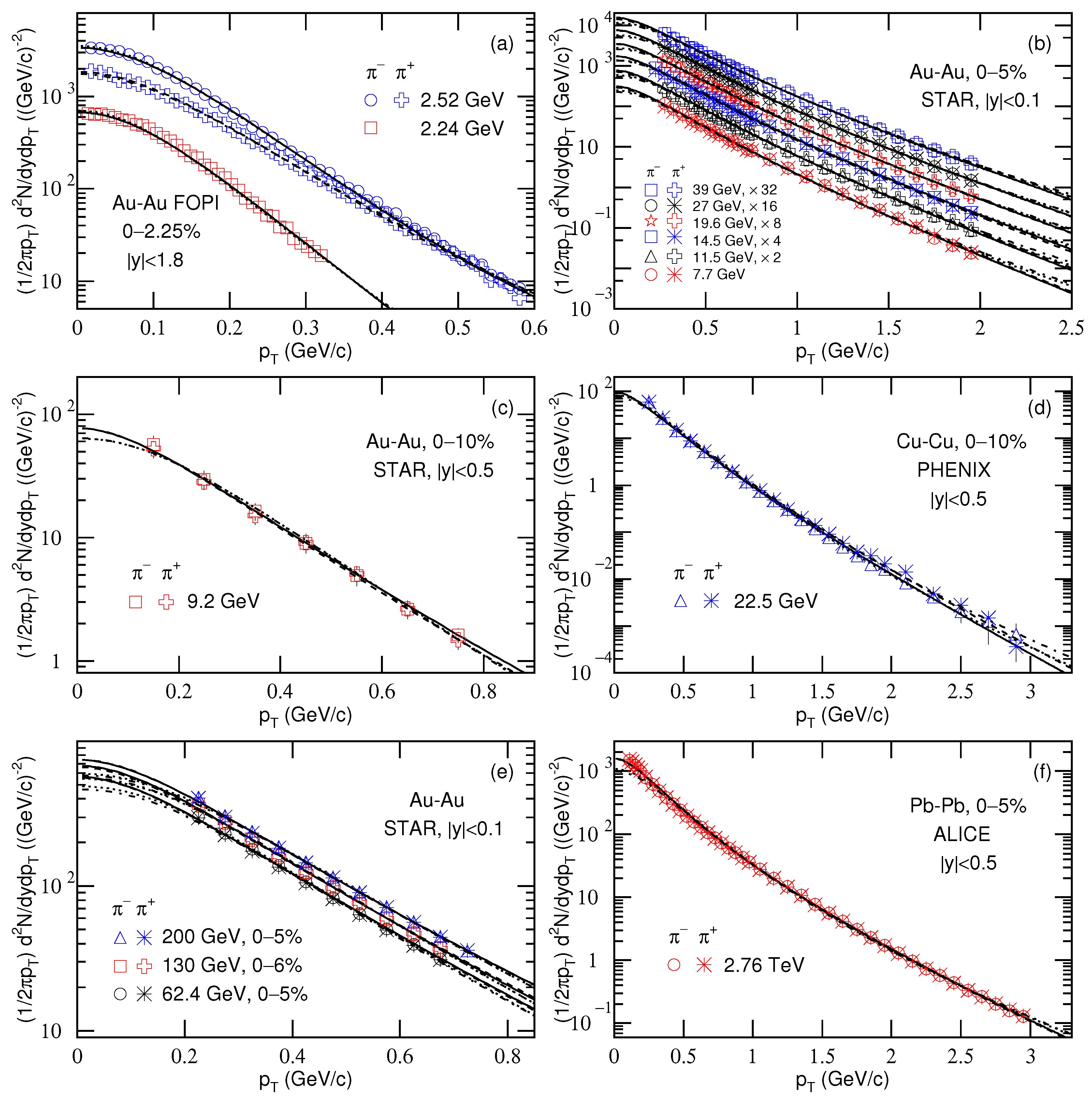
Figure A1 shows the spectra of and produced in mid-rapidity range in central Cu-Cu, Au-Au, and Pb-Pb collisions at high energies. Panels (a)–(f) represent the data by various symbols measured by the FOPI [81], STAR [55], STAR [7], PHENIX [82], STAR [6], and ALICE [20] Collaborations, respectively, where for 2.24 GeV Au-Au collisions in panel (a) only the spectrum of is available. As the same as Figure 1, the solid (dotted) curves are our results for () spectra fitted by Equation (7) through Equations (1) and (3), and the dashed (dot-dashed) curves are our results for () spectra fitted by Equation (7) through Equations (2) and (3), where only one set of parameters is used. The values of parameters are listed in Table A1 and Table A2 with and ndof, where the values of parameters are used directly in Figure 2 and indirectly in Figure 3. The fit results based on Equation (7) are well fitting to the experimental data measured in central collisions by the international collaborations [6,7,20,55,81,82].
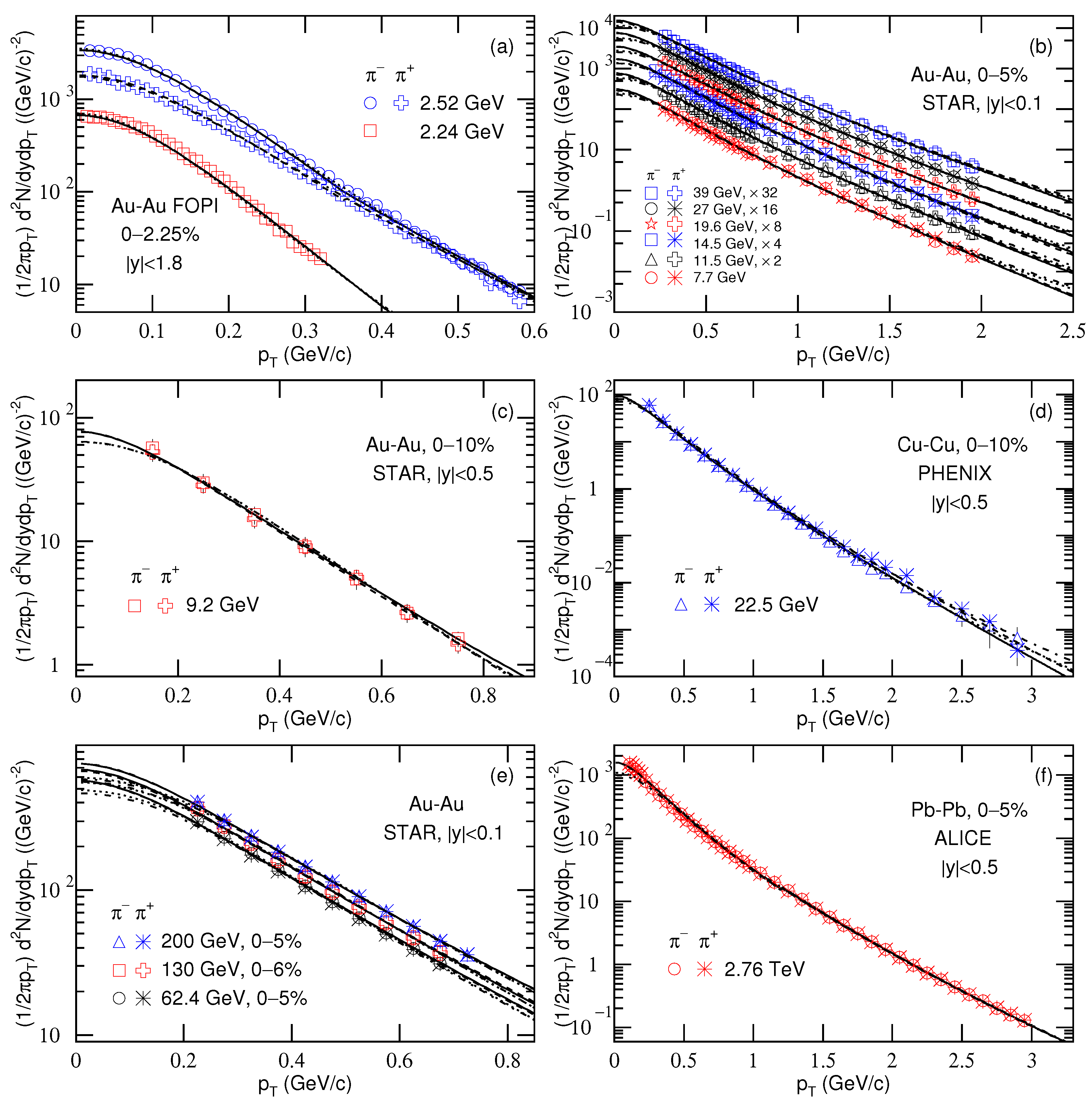
Figure A2 is the same as Figure A1, but it shows the fit results from Equation (8) through Equations (1) and (3) as well as through Equations (2) and (3). As the same as Figure 4, the solid (dotted) curves are the results for () spectra from Equation (8) through Equations (1) and (3), and the dashed (dot-dashed) curves are the results for () spectra from Equation (8) through Equations (2) and (3). The values of parameters are listed in Table A3 and Table A4 with and ndof, where the values of parameters are used directly in Figure 5 and indirectly in Figure 6. The fit results based on Equation (8) are well fitting to the experimental data measured in central collisions by the international collaborations [6,7,20,55,81,82]. It should be noted that Table A3 and Table A4 are nearly the same as Table A1 and Table A2 respectively, if not equal in error. The reason is that narrow ranges are used, in which the first component plays complete or main rule. The difference between Equations (7) and (8) is then not obvious.
Figure A1.
Same as Figure 1, but showing the results from central collisions. Panels (a–f) represent the data by various symbols measured by the FOPI [81], STAR [55], STAR [7], PHENIX [82], STAR [6], and ALICE [20] Collaborations, respectively.

Figure A2.
Same as Figure 4 and Figure A1, but showing the results from central collisions and Equation (8). Panels (a–f) represent the data by various symbols measured in different collisions by different Collaborations.


Table A1.
Values of , , k, , n, , , and ndof corresponding to the solid (dotted) curves for () spectra in Figure A1.
Table A1.
Values of , , k, , n, , , and ndof corresponding to the solid (dotted) curves for () spectra in Figure A1.
| Collab. | (GeV) | Part. | (MeV) | (c) | k | (GeV/c) | n | ndof | ||
|---|---|---|---|---|---|---|---|---|---|---|
| FOPI Au-Au | 2.24 | 1 | − | − | 38 | 33 | ||||
| 0–2.25% | 2.52 | 11 | 40 | |||||||
| 16 | 40 | |||||||||
| STAR Au-Au | 7.7 | 1 | − | − | 17 | 23 | ||||
| 0–5% | 1 | − | − | 27 | 23 | |||||
| 0–10% | 9.2 | 1 | − | − | 1 | 4 | ||||
| 1 | − | − | 1 | 4 | ||||||
| 0–5% | 11.5 | 1 | − | − | 4 | 23 | ||||
| 1 | − | − | 8 | 23 | ||||||
| 14.5 | 1 | − | − | 1 | 25 | |||||
| 1 | − | − | 1 | 25 | ||||||
| 19.6 | 1 | − | − | 3 | 23 | |||||
| 1 | − | − | 3 | 23 | ||||||
| 27 | 1 | − | − | 3 | 23 | |||||
| 1 | − | − | 3 | 23 | ||||||
| 39 | 1 | − | − | 4 | 23 | |||||
| 1 | − | − | 2 | 23 | ||||||
| 62.4 | 1 | − | − | 9 | 4 | |||||
| 1 | − | − | 9 | 4 | ||||||
| 0–6% | 130 | 1 | − | − | 25 | 4 | ||||
| 1 | − | − | 21 | 4 | ||||||
| 0–5% | 200 | 1 | − | − | 6 | 5 | ||||
| 1 | − | − | 9 | 5 | ||||||
| PHENIX Cu-Cu | 22.5 | 1 | − | − | 10 | 20 | ||||
| 0–10% | 1 | − | − | 13 | 20 | |||||
| ALICE Pb-Pb | 2760 | 37 | 35 | |||||||
| 0–5% | 37 | 35 |
Table A2.
Values of , , q, k, , n, , , and ndof corresponding to the dashed (dot-dashed) curves for () spectra in Figure A1.
Table A2.
Values of , , q, k, , n, , , and ndof corresponding to the dashed (dot-dashed) curves for () spectra in Figure A1.
| Collab. | (GeV) | Part. | (MeV) | (c) | q | k | (GeV/c) | n | ndof | ||
|---|---|---|---|---|---|---|---|---|---|---|---|
| FOPI Au-Au | 2.24 | 1 | − | − | 42 | 32 | |||||
| 0–2.25% | 2.52 | 1 | − | − | 5 | 42 | |||||
| 1 | − | − | 13 | 42 | |||||||
| STAR Au-Au | 7.7 | 1 | − | − | 31 | 22 | |||||
| 0–5% | 1 | − | − | 35 | 22 | ||||||
| 0–10% | 9.2 | 1 | − | − | 2 | 3 | |||||
| 1 | − | − | 2 | 3 | |||||||
| 0–5% | 11.5 | 1 | − | − | 18 | 22 | |||||
| 1 | − | − | 21 | 22 | |||||||
| 14.5 | 1 | − | − | 3 | 24 | ||||||
| 1 | − | − | 3 | 24 | |||||||
| 19.6 | 1 | − | − | 26 | 22 | ||||||
| 1 | − | − | 10 | 22 | |||||||
| 27 | 1 | − | − | 17 | 22 | ||||||
| 1 | − | − | 9 | 22 | |||||||
| 39 | 1 | − | − | 15 | 22 | ||||||
| 1 | − | − | 8 | 22 | |||||||
| 62.4 | 1 | − | − | 16 | 3 | ||||||
| 1 | − | − | 14 | 3 | |||||||
| 0–6% | 130 | 1 | − | − | 57 | 3 | |||||
| 1 | − | − | 49 | 3 | |||||||
| 0–5% | 200 | 1 | − | − | 20 | 4 | |||||
| 1 | − | − | 18 | 4 | |||||||
| PHENIX Cu-Cu | 22.5 | 1 | − | − | 8 | 19 | |||||
| 0–10% | 1 | − | − | 21 | 19 | ||||||
| ALICE Pb-Pb | 2760 | 88 | 34 | ||||||||
| 0–5% | 73 | 34 |
Table A3.
Values of , , k, , n, , , and ndof corresponding to the solid (dotted) curves for () spectra in Figure A2.
Table A3.
Values of , , k, , n, , , and ndof corresponding to the solid (dotted) curves for () spectra in Figure A2.
| Collab. | (GeV) | Part. | (MeV) | (c) | k | (GeV/c) | n | ndof | ||
|---|---|---|---|---|---|---|---|---|---|---|
| FOPI Au-Au | 2.24 | 1 | − | − | 38 | 33 | ||||
| 0–2.25% | 2.52 | 11 | 39 | |||||||
| 16 | 39 | |||||||||
| STAR Au-Au | 7.7 | 1 | − | − | 17 | 23 | ||||
| 0–5% | 1 | − | − | 27 | 23 | |||||
| 0–10% | 9.2 | 1 | − | − | 1 | 4 | ||||
| 1 | − | − | 1 | 4 | ||||||
| 0–5% | 11.5 | 1 | − | − | 4 | 23 | ||||
| 1 | − | − | 8 | 23 | ||||||
| 14.5 | 1 | − | − | 1 | 25 | |||||
| 1 | − | − | 1 | 25 | ||||||
| 19.6 | 1 | − | − | 3 | 23 | |||||
| 1 | − | − | 3 | 23 | ||||||
| 27 | 1 | − | − | 3 | 23 | |||||
| 1 | − | − | 3 | 23 | ||||||
| 39 | 1 | − | − | 4 | 23 | |||||
| 1 | − | − | 2 | 23 | ||||||
| 62.4 | 1 | − | − | 9 | 4 | |||||
| 1 | − | − | 9 | 4 | ||||||
| 0–6% | 130 | 1 | − | − | 25 | 4 | ||||
| 1 | − | − | 21 | 4 | ||||||
| 0–5% | 200 | 1 | − | − | 6 | 5 | ||||
| 1 | − | − | 9 | 5 | ||||||
| PHENIX Cu-Cu | 22.5 | 1 | − | − | 10 | 20 | ||||
| 0–10% | 1 | − | − | 13 | 20 | |||||
| ALICE Pb-Pb | 2760 | 37 | 35 | |||||||
| 0–5% | 37 | 35 |
Table A4.
Values of , , q, k, , n, , , and ndof corresponding to the dashed (dot-dashed) curves for () spectra in Figure A2.
Table A4.
Values of , , q, k, , n, , , and ndof corresponding to the dashed (dot-dashed) curves for () spectra in Figure A2.
| Collab. | (GeV) | Part. | (MeV) | (c) | q | k | (GeV/c) | n | ndof | ||
|---|---|---|---|---|---|---|---|---|---|---|---|
| FOPI Au-Au | 2.24 | 1 | − | − | 42 | 32 | |||||
| 0–2.25% | 2.52 | 1 | − | − | 5 | 42 | |||||
| 1 | − | − | 13 | 42 | |||||||
| STAR Au-Au | 7.7 | 1 | − | − | 31 | 22 | |||||
| 0–5% | 1 | − | − | 35 | 22 | ||||||
| 0–10% | 9.2 | 1 | − | − | 2 | 3 | |||||
| 1 | − | − | 2 | 3 | |||||||
| 0–5% | 11.5 | 1 | − | − | 18 | 22 | |||||
| 1 | − | − | 21 | 22 | |||||||
| 14.5 | 1 | − | − | 3 | 24 | ||||||
| 1 | − | − | 3 | 24 | |||||||
| 19.6 | 1 | − | − | 26 | 22 | ||||||
| 1 | − | − | 10 | 22 | |||||||
| 27 | 1 | − | − | 17 | 22 | ||||||
| 1 | − | − | 9 | 22 | |||||||
| 39 | 1 | − | − | 15 | 22 | ||||||
| 1 | − | − | 8 | 22 | |||||||
| 62.4 | 1 | − | − | 16 | 3 | ||||||
| 1 | − | − | 14 | 3 | |||||||
| 0–6% | 130 | 1 | − | − | 57 | 3 | |||||
| 1 | − | − | 49 | 3 | |||||||
| 0–5% | 200 | 1 | − | − | 20 | 4 | |||||
| 1 | − | − | 18 | 4 | |||||||
| PHENIX Cu-Cu | 22.5 | 1 | − | − | 8 | 19 | |||||
| 0–10% | 1 | − | − | 21 | 19 | ||||||
| ALICE Pb-Pb | 2760 | 88 | 34 | ||||||||
| 0–5% | 73 | 34 |
References
- Cleymans, J.; Oeschler, H.; Redlich, K.; Wheaton, S. Comparison of chemical freeze-out criteria in heavy-ion collisions. Phys. Rev. C 2006, 73, 034905. [Google Scholar] [CrossRef]
- Andronic, A.; Braun-Munzinger, P.; Stachel, J. Thermal hadron production in relativistic nuclear collisions. Acta Phys. Pol. B 2009, 40, 1005–1012. [Google Scholar]
- Andronic, A.; Braun-Munzinger, P.; Stachel, J. The horn, the hadron mass spectrum and the QCD phase diagram: The statistical model of hadron production in central nucleus-nucleus collisions. Nucl. Phys. A 2010, 834, 237c–240c. [Google Scholar] [CrossRef] [Green Version]
- Hama, Y.; Navarra, F.S. Energy and mass number dependence of the dissociation temperature in hydrodynamical models. Z. Phys. C 1992, 53, 501–506. [Google Scholar] [CrossRef]
- Schnedermann, E.; Sollfrank, J.; Heinz, U. Thermal phenomenology of hadrons from 200A GeV S + S collisions. Phys. Rev. C 1993, 48, 2462–2475. [Google Scholar] [CrossRef] [Green Version]
- Abelev, B.I.; et al. [STAR Collaboration] Systematic measurements of identified particle spectra in pp, d + Au, and Au + Au collisions at the STAR detector. Phys. Rev. C 2009, 79, 034909. [Google Scholar] [CrossRef]
- Abelev, B.I.; et al. [STAR Collaboration] Identified particle production, azimuthal anisotropy, and interferometry measurements in Au+Au collisions at = 9.2 GeV. Phys. Rev. C 2010, 81, 024911. [Google Scholar] [CrossRef]
- Tang, Z.B.; Xu, Y.C.; Ruan, L.J.; Van Buren, G.; Wang, F.Q.; Xu, Z.B. Spectra and radial flow at RHIC with Tsallis statistics in a blast-wave description. Phys. Rev. C 2009, 79, 051901(R). [Google Scholar] [CrossRef] [Green Version]
- Tang, Z.B.; Li, Y.; Ruan, L.J.; Shao, M.; Chen, H.F.; Li, C.; Mohanty, B.; Sorensen, P.; Tang, A.H.; Xu, Z.B. Statistical origin of constituent-quark scaling in the QGP hadronization. Chin. Phys. Lett. 2013, 30, 031201. [Google Scholar] [CrossRef] [Green Version]
- Jiang, K.; Zhu, Y.Y.; Liu, W.T.; Chen, H.F.; Li, C.; Ruan, L.J.; Tang, Z.B.; Xu, Z.B. Onset of radial flow in p+p collisions. Phys. Rev. C 2015, 91, 024910. [Google Scholar] [CrossRef] [Green Version]
- Takeuchi, S.; Murase, K.; Hirano, T.; Huovinen, P.; Nara, Y. Effects of hadronic rescattering on multistrange hadrons in high-energy nuclear collisions. Phys. Rev. C 2015, 92, 044907. [Google Scholar] [CrossRef] [Green Version]
- Heiselberg, H.; Levy, A.M. Elliptic flow and HBT in noncentral nuclear collisions. Phys. Rev. C 1999, 59, 2716–2727. [Google Scholar] [CrossRef] [Green Version]
- Heinz, U.W. Concepts of heavy-ion physics. arXiv 2003, arXiv:hep-ph/0407360. [Google Scholar]
- Russo, R. Measurement of D+ Meson Production in p-Pb Collisions with the ALICE Detector. Ph.D. Thesis, Universita degli Studi di Torino, Torino, Italy, 2015. [Google Scholar]
- Wei, H.-R.; Liu, F.-H.; Lacey, R.A. Kinetic freeze-out temperature and flow velocity extracted from transverse momentum spectra of final-state light flavor particles produced in collisions at RHIC and LHC. Eur. Phys. J. A 2016, A52, 102. [Google Scholar] [CrossRef] [Green Version]
- Lao, H.-L.; Wei, H.-R.; Liu, F.-H.; Lacey, R.A. An evidence of mass-dependent differential kinetic freeze-out scenario observed in Pb-Pb collisions at 2.76 TeV. Eur. Phys. J. A 2016, 52, 203. [Google Scholar] [CrossRef] [Green Version]
- Wei, H.-R.; Liu, F.-H.; Lacey, R.A. Disentangling random thermal motion of particles and collective expansion of source from transverse momentum spectra in high energy collisions. J. Phys. G 2016, 43, 125102. [Google Scholar] [CrossRef] [Green Version]
- Lao, H.-L.; Liu, F.-H.; Li, B.-C.; Duan, M.-Y. Kinetic freeze-out temperatures in central and peripheral collisions: Which one is larger? Nucl. Sci. Tech. 2018, 29, 82. [Google Scholar] [CrossRef] [Green Version]
- Andronic, A. An overview of the experimental study of quark-gluon matter in high-energy nucleus-nucleus collisions. Int. J. Mod. Phys. A 2014, 29, 1430047. [Google Scholar] [CrossRef] [Green Version]
- Abelev, B.; et al. [ALICE Collaboration] Pion, kaon, and proton production in central Pb–Pb collisions at = 2.76 TeV. Phys. Rev. Lett. 2012, 109, 252301. [Google Scholar] [CrossRef] [Green Version]
- Zhang, S.; Ma, Y.G.; Chen, J.H.; Zhong, C. Production of kaon and Λ in nucleus-nucleus collisions at ultrarelativistic energy from a blast-wave model. Adv. High Energy Phys. 2015, 2015, 460590. [Google Scholar] [CrossRef]
- Das, S. Identified particle production and freeze-out properties in heavy-ion collisions at RHIC beam energy scan program. In EPJ Web of Conferences; EDP Sciences: Jules, France, 2015; Volume 90, p. 08007. [Google Scholar]
- Das, S.; et al. [STAR Collaboration] Centrality dependence of freeze-out parameters from the beam energy scan at STAR. Nucl. Phys. A 2013, 904–905, 891c–894c. [Google Scholar]
- Abgrall, N.; et al. [NA61/SHINE Collaboration] Measurement of negatively charged pion spectra in inelastic p+p interactions at plab = 20, 31, 40, 80 and 158 GeV/c. Eur. Phys. J. C 2014, 74, 2794. [Google Scholar] [CrossRef] [Green Version]
- Adare, A.; et al. [PHENIX Collaboration] Identified charged hadron production in p+p collisions at = 200 and 62.4 GeV. Phys. Rev. C 2011, 83, 064903. [Google Scholar] [CrossRef]
- Aamodt, K.; et al. [ALICE Collaboration] Production of pions, kaons and protons in pp collisions at = 900 GeV with ALICE at the LHC. Eur. Phys. J. C 2011, 71, 1655. [Google Scholar] [CrossRef] [Green Version]
- Chatrchyan, S.; et al. [CMS Collaboration] Study of the inclusive production of charged pions, kaons, and protons in pp collisions at = 0.9, 2.76, and 7 TeV. Eur. Phys. J. C 2012, 72, 2164. [Google Scholar] [CrossRef] [Green Version]
- Sirunyan, A.M.; et al. [CMS Collaboration] Measurement of charged pion, kaon, and proton production in proton-proton collisions at = 13 TeV. Phys. Rev. D 2017, 96, 112003. [Google Scholar] [CrossRef] [Green Version]
- Petrovici, M.; Andrei, C.; Berceanu, I.; Bercuci, A.; Herghelegiu, A.; Pop, A. Recent results and open questions on collective type phenomena from A-A to pp collisions. AIP Conf. Proc. 2015, 1645, 52. [Google Scholar]
- Cleymans, J.; Worku, D. Relativistic thermodynamics: Transverse momentum distributions in high-energy physics. Eur. Phys. J. A 2012, 48, 160. [Google Scholar] [CrossRef]
- Zheng, H.; Zhu, L.L. Comparing the Tsallis distribution with and without tthermodynamical description in p + p collisions. Adv. High Energy Phys. 2016, 2016, 9632126. [Google Scholar] [CrossRef] [Green Version]
- Odorico, R. Does a transverse energy trigger actually trigger on large-PT jets? Phys. Lett. B 1982, 118, 151–154. [Google Scholar] [CrossRef]
- Arnison, G.; et al. [UA1 Collaboration] Transverse momentum spectra for charged particles at the CERN proton-antiproton collider. Phys. Lett. B 1982, 118, 167–172. [Google Scholar] [CrossRef] [Green Version]
- Mizoguchi, T.; Biyajima, M.; Suzuki, N. Analyses of whole transverse momentum distributions in pp and pp collisions by using a modified version of Hagedorn’s formula. Int. J. Mod. Phys. A 2017, 32, 1750057. [Google Scholar] [CrossRef] [Green Version]
- Hagedorn, R. Multiplicities, pT distributions and the expected hadron⟶quark-gluon phase transition. Riv. Nuovo Cimento 1983, 6, 1. [Google Scholar] [CrossRef]
- Abelev, B.; et al. [ALICE Collaboration] Production of Σ(1385)± and Ξ(1530)0 in proton-proton collisions at = 7 TeV. Eur. Phys. J. C 2015, 75, 1. [Google Scholar]
- Aamodt, K.; et al. [ALICE Collaboration] Transverse momentum spectra of charged particles in proton-proton collisions at = 900 GeV with ALICE at the LHC. Phys. Lett. B 2010, 693, 53–68. [Google Scholar] [CrossRef] [Green Version]
- De Falco, A.; et al. [ALICE Collaboration] Vector meson production in pp collisions at = 7 TeV, measured with the ALICE detector. J. Phys. G 2011, 38, 124083. [Google Scholar] [CrossRef]
- Abelev, B; et al. [ALICE Collaboration] Light vector meson production in pp collisions at = 7 TeV. Phys. Lett. B 2012, 710, 557–568. [Google Scholar] [CrossRef]
- Abt, I.; et al. [HERA-B Collaboration] K*0 and ψ meson production in proton-nucleus interactions at = 41.6 GeV. Eur. Phys. J. C 2007, 50, 315–328. [Google Scholar] [CrossRef]
- Abelev, B.; et al. [ALICE Collaboration] Inclusive J/ψ production in pp collisions at = 2.76 TeV. Phys. Lett. B 2012, 718, 295–306, and Erratum Phys. Lett. B 2015, 748, 472–473. [Google Scholar] [CrossRef] [Green Version]
- Lakomov, I.; et al. [ALICE Collaboration] Event activity dependence of inclusive J/ψ production in p-Pb collisions at = 5.02 TeV with ALICE at the LHC. Nucl. Phys. A 2014, 931, 1179–1183. [Google Scholar] [CrossRef] [Green Version]
- Abelev, B.; et al. [ALICE Collaboration] Heavy flavour decay muon production at forward rapidity in proton-proton collisions at = 7 TeV. Phys. Lett. B 2012, 708, 265–275. [Google Scholar] [CrossRef]
- Aad, G.; et al. [ATLAS Collaboration] Charged-particle multiplicities in pp interactions at = 900 GeV with the ATLAS detector at the LHC. Phys. Lett. B 2010, 688, 21–42. [Google Scholar] [CrossRef]
- Aad, G.; et al. [ATLAS Collaboration] Charged-particle multiplicities in pp interactions measured with the ATLAS detector at the LHC. New J. Phys. 2011, 13, 053033. [Google Scholar] [CrossRef] [Green Version]
- Aad, G.; et al. [ATLAS Collaboration] Measurement of charged-particle spectra in Pb+Pb collisions at = 2.76 TeV with the ATLAS detector at the LHC. J. High Energy Phys. 2015, 2015, 050. [Google Scholar] [CrossRef] [Green Version]
- Aad, G.; et al. [ATLAS Collaboration] Charged-particle distributions in = 13 TeV pp interactions measured with the ATLAS detector at the LHC. Phys. Lett. B 2016, 758, 67–88. [Google Scholar] [CrossRef] [Green Version]
- Aad, G.; et al. [ATLAS Collaboration] Charged-particle distributions in pp interactions at = 8 TeV measured with the ATLAS detector. Eur. Phys. J. C 2016, 76, 403. [Google Scholar] [CrossRef] [PubMed] [Green Version]
- Avdyushev, V.A. A new method for the statistical simulation of the virtual values of parameters in inverse orbital dynamics problems. Sol. Syst. Res. 2009, 43, 543. [Google Scholar] [CrossRef]
- Liu, F.-H.; Gao, Y.-Q.; Wei, H.-R. On descriptions of particle transverse momentum spectra in high energy collisions. Adv. High Energy Phys. 2014, 2014, 293873. [Google Scholar] [CrossRef] [Green Version]
- Cleymans, J. The physics case for the ≈ 10 GeV energy region. In Walter Greiner Memorial Volume; Hess, P.O., Ed.; World Scientiflc: Singapore, 2018. [Google Scholar]
- Bjorken, J.D. Highly relativistic nucleus-nucleus collisions: The central rapidity region. Phys. Rev. D 1983, 27, 140–151. [Google Scholar] [CrossRef]
- Okamoto, K.; Nonaka, C. A new relativistic viscous hydrodynamics code and its application to the Kelvin-Helmholtz instability in high-energy heavy-ion collisions. Eur. Phys. J. C 2017, 77, 383. [Google Scholar] [CrossRef]
- Zhang, S.; Ma, Y.G.; Chen, J.H.; Zhong, C. Beam energy dependence of Hanbury-Brown-Twiss radii from a blast-wave model. Adv. High Energy Phys. 2016, 2016, 9414239. [Google Scholar] [CrossRef]
- Adamczyk, L.; et al. [STAR Collaboration] Bulk properties of the medium produced in relativistic heavy-ion collisions from the beam energy scan program. Phys. Rev. C 2017, 96, 044904. [Google Scholar] [CrossRef] [Green Version]
- Luo, X.F. Exploring the QCD phase structure with beam energy scan in heavy-ion collisions. Nucl. Phys. A 2016, 956, 75–82. [Google Scholar] [CrossRef] [Green Version]
- Chatterjee, S.; Das, S.; Kumar, L.; Mishra, D.; Mohanty, B.; Sahoo, R.; Sharma, N. Freeze-out parameters in heavy-ion collisions at AGS, SPS, RHIC, and LHC energies. Adv. High Energy Phys. 2015, 2015, 349013. [Google Scholar] [CrossRef]
- Acharya, S.; et al. [ALICE Collaboration] Multiplicity dependence of light-flavor hadron production in pp collisions at = 7 TeV. Phys. Rev. C 2019, 99, 024906. [Google Scholar] [CrossRef] [Green Version]
- Gutay, L.G.; Hirsch, A.S.; Pajares, C.; Scharenberg, R.P.; Srivastava, B.K. De-confinement in small systems: Clustering of color sources in high multiplicity pp collisions at = 1.8 TeV. Int. J. Mod. Phys. E 2015, 24, 1550101. [Google Scholar] [CrossRef] [Green Version]
- Hirsch, A.S.; Pajares, C.; Scharenberg, R.P.; Srivastava, B.K. De-confinement in high multiplicity proton-proton collisions at LHC energies. arXiv 2018, arXiv:1803.02301 [hep-ph]. [Google Scholar]
- Sahoo, P.; De, S.; Tiwari, S.K.; Sahoo, R. Energy and centrality dependent study of deconfinement phase transition in a color string percolation approach at RHIC energies. Eur. Phys. J. A 2018, 54, 136. [Google Scholar] [CrossRef] [Green Version]
- Li, L.L.; Liu, F.-H. Energy dependent kinetic freeze-out temperature and transverse flow velocity in high energy collisions. Eur. Phys. J. A 2018, 54, 169. [Google Scholar] [CrossRef] [Green Version]
- Sarkisyan, E.K.G.; Sakharov, A.S. On similarities of bulk observables in nuclear and particle collisions. CERN-PH-TH-2004-213. arXiv 2004, arXiv:hep-ph/0410324. [Google Scholar]
- Sarkisyan, E.K.G.; Sakharov, A.S. Multihadron production features in different reactions. AIP Conf. Proc. 2006, 828, 35. [Google Scholar]
- Back, B.B.; et al. [PHOBOS Collaboration] Centrality and energy dependence of charged-particle multiplicities in heavy ion collisions in the context of elementary reactions. Phys. Rev. C 2006, 74, 021902(R). [Google Scholar] [CrossRef]
- Lao, H.-L.; Liu, F.-H.; Li, B.-C.; Duan, M.-Y.; Lacey, R.A. Examining the model dependence of the determination of kinetic freeze-out temperature and transverse flow velocity in small collision system. Nucl. Sci. Tech. 2018, 29, 164. [Google Scholar] [CrossRef] [Green Version]
- Song, H.C.; Zhou, Y.; Gajdošová, K. Collective flow and hydrodynamics in large and small systems at the LHC. Nucl. Sci. Tech. 2017, 28, 99. [Google Scholar] [CrossRef] [Green Version]
- He, X.-W.; Wei, H.-R.; Liu, F.-H. Chemical potentials of light hadrons and quarks from yield ratios of negative to positive particles in high energy pp collisions. J. Phys. G 2019, 46, 025102. [Google Scholar] [CrossRef] [Green Version]
- Tsallis, C. Possible generalization of Boltzmann-Gibbs statistics. J. Stat. Phys. 1988, 52, 479–487. [Google Scholar] [CrossRef]
- Biró, T.S.; Purcsel, G.; Ürmössy, K. Non-extensive approach to quark matter. Eur. Phys. J. A 2009, 40, 325. [Google Scholar]
- Sjöstrand, T. High-energy physics event generation with PYTHIA 5.7 and JETSET 7.4. Comput. Phys. Commun. 1994, 82, 74–90. [Google Scholar] [CrossRef] [Green Version]
- Sjöstrand, T.; Mrenna, S.; Skands, P.Z. A brief introduction to PYTHIA 8.1. Comput. Phys. Commun. 2008, 178, 852–867. [Google Scholar] [CrossRef] [Green Version]
- Skands, P.; Carrazza, S.; Rojo, J. Tuning PYTHIA 8.1: The Monash 2013 tune. Eur. Phys. J. C 2014, 74, 3024. [Google Scholar] [CrossRef] [Green Version]
- Sjöstrand, T.; Mrenna, S.; Skands, P. PYTHIA 6.4 physics and manual. J. High Energy Phys. 2006, 2006, 026. [Google Scholar] [CrossRef]
- Trainor, T.A. Comparing the PYTHIA Monte Carlo to a two-component (soft + hard) model of hadron production in high-energy p-p collisions. Int. J. Mod. Phys. E 2019, 28, 1950023. [Google Scholar] [CrossRef] [Green Version]
- Tawfik, A.N.; Yassin, H.; Abo Elyazeed, E.R. On thermodynamic self-consistency of generic axiomatic-nonextensive statistics. Chin. Phys. C 2017, 41, 053107. [Google Scholar] [CrossRef] [Green Version]
- Tawfik, A.N. Lattice QCD thermodynamics and RHIC-BES particle production within generic nonextensive statistics. Phys. Part. Nucl. Lett. 2018, 15, 199–209. [Google Scholar] [CrossRef] [Green Version]
- Tawfik1, A.; Yassin, H.; Abo Elyazeed, E.R. Chemical freezeout parameters within generic nonextensive statistics. Indian J. Phys. 2018, 92, 1325–1335. [Google Scholar] [CrossRef] [Green Version]
- Tawfik, A.N. Baryon-to-pion ratios within generic (non)extensive statistics. PoS 2016, ICHEP2016, 1153. [Google Scholar]
- Sahu, D.; Tripathy, S.; Pradhan, G.S.; Sahoo, R. Role of event multiplicity on hadronic phase lifetime and QCD phase boundary in ultrarelativistic collisions at energies available at the BNL Relativistic Heavy Ion Collider and CERN Large Hadron Collider. Phys. Rev. C 2020, 101, 014902. [Google Scholar] [CrossRef] [Green Version]
- Reisdorf, W.; et al. [FOPI Collaboration] Systematics of pion emission in heavy ion collisions in the 1A GeV regime. Nucl. Phys. A 2007, 781, 459–508. [Google Scholar] [CrossRef] [Green Version]
- Mitchell, J.T.; et al. [STAR Collaboration] RHIC critical point search: Assessing STAR’s capabilities. PoS 2007, CPOD2006, 019. [Google Scholar]
Figure 1.
Transverse momentum spectra of and produced at mid-(pseudo)rapidity in collisions at high energies, where the mid-(pseudo)rapidity intervals and energies are marked in the panels. The symbols presented in panels (a–e) represent the data of NA61/SHINE [24], PHENIX [25], STAR [6], ALICE [26], and CMS [27,28] Collaborations, respectively, where in panel (a) only the spectra of are available, and panel (c) is for NSD events and other panels are for INEL events. Although the collisions are divided on the multiplicity classes in experiments on the LHC, we have used the minimum-bias INEL events [26,27,28]. In some cases, different amounts marked in the panels are used to scale the data for clarity. The blue solid (dotted) curves are our results for () spectra fitted by Equation (7) through Equations (1) and (3), and the blue dashed (dot-dashed) curves are our results for () spectra fitted by Equation (7) through Equations (2) and (3), by the first set of parameter values. The results by the second set of parameters (if available) are presented by the black curves.

Figure 2.
Excitation functions of (a) , (b) , (c) , (d) n, and (e) k. The closed (open) symbols represent the parameter values corresponding to () spectra, which are listed in Table 1 and Table 2. The blue circles (black squares) represent the first set of parameter values obtained from Equation (7) through Equations (1)–(3). The blue asterisks (black triangles) represent the second set of parameter values obtained from Equation (7) through Equations (1)–(3). The red asterisks (green triangles) represent the parameter values from collisions for comparisons, which are listed in Table A1 and Table A2 in the Appendix A.

Figure 3.
Excitation functions of (a,b) and (c,d) . The open symbols (open symbols with asterisks) represent the values corresponding to () spectra. The blue circles (black squares) represent the results obtained indirectly from Equations (1) and (2) for the left panel, or from Equation (7) through Equations (1)–(3) for the right panel, by the first set of parameter values. The results by the second set of parameter values are presented by the blue asterisks (black triangles). These values are indirectly obtained according to the parameter values listed in Table 1 and Table 2. The lines are the fitted results for various symbols for collisions. The red asterisks (green triangles) represent the results from collisions for comparisons, which are indirectly obtained according to the parameter values listed in Table A1 and Table A2 in the Appendix A.

Figure 4.
Same as Figure 1, but showing the results fitted by Equation (8) through Equations (1) and (3) with one set of parameter values and by Equation (8) through Equations (2) and (3) with two sets of parameter values, where in panel (a) only the spectra of are available, and panel (c) is for NSD events and panels (b,d,e) are for INEL events. The blue solid (dotted) curves are the results for () spectra fitted by Equation (8) through Equations (1) and (3), and the blue and black dashed (dot-dashed) curves are the results for () spectra fitted by Equation (8) through Equations (2) and (3).

Figure 5.
Same as Figure 2, but showing the results obtained from Equation (8) through Equations (1) and (3) with one set of parameter values and from Equation (8) through Equations (2) and (3) with two sets of parameter values, where the excitation functions of , , , n, and k are presented in panels (a–e), respectively. The blue circles represent the parameter values obtained from Equation (8) through Equations (1) and (3). black The squares (triangles) represent the first (second) set of parameter values obtained from Equation (8) through Equations (2) and (3). The related parameter values are listed in Table 3 and Table 4. The red asterisks (green triangles) represent the parameter values from collisions for comparisons, which are listed in Table A3 and Table A4 in the Appendix A.

Figure 6.
Same as Figure 3, but showing the results obtained from Equations (1) and (2) for the left panel, or from Equation (8) through Equations (1)–(3) for the right panel, where the excitation functions of and are presented in panels (a–d) respectively. The circles represent the results obtained indirectly from Equation (1) for the left panel, or from Equation (8) through Equations (1) and (3) for the right panel, by the parameter values. The squares (triangles) represent the results obtained indirectly from Equation (2) for the left panel, or from Equation (8) through Equations (2) and (3) for the right panel, by the first (second) set of parameter values. These values are indirectly obtained according to the parameter values listed in Table 3 and Table 4. The red asterisks (green triangles) represent the results from collisions for comparisons, which are indirectly obtained according to the parameter values listed in Table A3 and Table A4 in the Appendix A.

Table 1.
Values of free parameters (, , k, , and n), normalization constant (), , and ndof corresponding to the solid (dotted) curves for () spectra in Figure 1 in which different data are measured in different mid-(pseudo)rapidity intervals at different energies by different Collaborations. The values presented in terms of value/value denote respectively the first and second sets of parameter values in Equation (7) through Equations (1) and (3) in which .
| Collab. | (GeV) | Part. | (MeV) | (c) | k | (GeV/c) | n | ndof | ||
|---|---|---|---|---|---|---|---|---|---|---|
| NA61/ | 6.3 | 1 | − | − | 21 | 15 | ||||
| SHINE | 7.7 | 1 | − | − | 34 | 15 | ||||
| INEL | 8.8 | 1 | − | − | 73 | 15 | ||||
| 12.3 | 1 | − | − | 59 | 15 | |||||
| 17.3 | 1 | − | − | 26 | 15 | |||||
| PHENIX | 62.4 | 7/28 | 20 | |||||||
| INEL | 11/11 | 20 | ||||||||
| 200 | 26/21 | 21 | ||||||||
| 54/26 | 21 | |||||||||
| STAR | 200 | 76/3 | 6 | |||||||
| NSD | 96/4 | 6 | ||||||||
| ALICE | 900 | 38/126 | 27 | |||||||
| INEL | 49/137 | 27 | ||||||||
| CMS | 900 | 24/62 | 16 | |||||||
| INEL | 16/59 | 16 | ||||||||
| 2760 | 34/70 | 16 | ||||||||
| 35/74 | 16 | |||||||||
| 7000 | 48/67 | 16 | ||||||||
| 55/70 | 16 | |||||||||
| 13000 | 30/28 | 16 | ||||||||
| 36/42 | 16 |
Table 2.
Values of free parameters (, , qk, , and n), normalization constant (), , and ndof corresponding to the dashed (dot-dashed) curves for () spectra in Figure 1 in which different data are measured in different mid-(pseudo)rapidity intervals at different energies by different Collaborations. The values presented in terms of value/value denote respectively the first and second sets of parameter values in Equation (7) through Equations (2) and (3) in which .
| Collab. | (GeV) | Part. | (MeV) | (c) | q | (GeV/c) | n | ndof | |||
|---|---|---|---|---|---|---|---|---|---|---|---|
| NA61/ | 6.3 | 1 | − | − | 12 | 14 | |||||
| SHINE | 7.7 | 1 | − | − | 13 | 14 | |||||
| INEL | 8.8 | 1 | − | − | 24 | 14 | |||||
| 12.3 | 1 | − | − | 14 | 14 | ||||||
| 17.3 | 1 | − | − | 5 | 14 | ||||||
| PHENIX | 62.4 | 16/18 | 19 | ||||||||
| INEL | 30/23 | 19 | |||||||||
| 200 | 39/24 | 20 | |||||||||
| 45/68 | 20 | ||||||||||
| STAR | 200 | 22/39 | 5 | ||||||||
| NSD | 15/28 | 5 | |||||||||
| ALICE | 900 | 34/419 | 26 | ||||||||
| INEL | 51/558 | 26 | |||||||||
| CMS | 900 | 8/124 | 15 | ||||||||
| INEL | 6/121 | 15 | |||||||||
| 2760 | 15/114 | 15 | |||||||||
| 15/115 | 15 | ||||||||||
| 7000 | 23/129 | 15 | |||||||||
| 31/171 | 15 | ||||||||||
| 13000 | 13/50 | 15 | |||||||||
| 27/74 | 15 |
Table 3.
Values of , , k, , n, , , and ndof corresponding to the solid (dotted) curves for () spectra in Figure 4, where Equation (8) through Equations (1) and (3) is used.
| Collab. | (GeV) | Part. | (MeV) | (c) | k | (GeV/c) | n | ndof | ||
|---|---|---|---|---|---|---|---|---|---|---|
| NA61/ | 6.3 | 1 | − | − | 24 | 15 | ||||
| SHINE | 7.7 | 1 | − | − | 44 | 15 | ||||
| INEL | 8.8 | 1 | − | − | 86 | 15 | ||||
| 12.3 | 1 | − | − | 78 | 15 | |||||
| 17.3 | 1 | − | − | 34 | 15 | |||||
| PHENIX | 62.4 | 9 | 20 | |||||||
| INEL | 18 | 20 | ||||||||
| 200 | 16 | 21 | ||||||||
| 26 | 21 | |||||||||
| STAR | 200 | 1 | − | − | 2 | 6 | ||||
| NSD | 1 | − | − | 6 | 6 | |||||
| ALICE | 900 | 101 | 27 | |||||||
| INEL | 131 | 27 | ||||||||
| CMS | 900 | 47 | 16 | |||||||
| INEL | 43 | 16 | ||||||||
| 2760 | 57 | 16 | ||||||||
| 76 | 16 | |||||||||
| 7000 | 73 | 16 | ||||||||
| 90 | 16 | |||||||||
| 13000 | 31 | 16 | ||||||||
| 57 | 16 |
Table 4.
Values of , , q, k, , n, , , and ndof corresponding to the dashed (dot-dashed) curves for () spectra in Figure 4, where Equation (8) through Equations (2) and (3) is used.
| Collab. | (GeV) | Part. | (MeV) | (c) | q | k | (GeV/c) | n | ndof | ||
|---|---|---|---|---|---|---|---|---|---|---|---|
| NA61/ | 6.3 | 1 | − | − | 11 | 14 | |||||
| SHINE | 7.7 | 1 | − | − | 8 | 14 | |||||
| INEL | 8.8 | 1 | − | − | 23 | 14 | |||||
| 12.3 | 1 | − | − | 11 | 14 | ||||||
| 17.3 | 1 | − | − | 4 | 14 | ||||||
| PHENIX | 62.4 | 33/39 | 18 | ||||||||
| INEL | 15/15 | 18 | |||||||||
| 200 | 16/31 | 19 | |||||||||
| 26/32 | 19 | ||||||||||
| STAR | 200 | 1 | − | − | 34 | 5 | |||||
| NSD | 1 | − | − | 38 | 5 | ||||||
| ALICE | 900 | 187/287 | 25 | ||||||||
| INEL | 232/333 | 25 | |||||||||
| CMS | 900 | 79/95 | 14 | ||||||||
| INEL | 70/72 | 14 | |||||||||
| 2760 | 70/72 | 14 | |||||||||
| 87/88 | 14 | ||||||||||
| 7000 | 68/69 | 14 | |||||||||
| 87/92 | 14 | ||||||||||
| 13000 | 34/39 | 14 | |||||||||
| 56/59 | 14 |
© 2020 by the authors. Licensee MDPI, Basel, Switzerland. This article is an open access article distributed under the terms and conditions of the Creative Commons Attribution (CC BY) license (http://creativecommons.org/licenses/by/4.0/).
Share and Cite
MDPI and ACS Style
Li, L.-L.; Liu, F.-H. Kinetic Freeze-Out Properties from Transverse Momentum Spectra of Pions in High Energy Proton-Proton Collisions. Physics 2020, 2, 277-308. https://0-doi-org.brum.beds.ac.uk/10.3390/physics2020015
AMA Style
Li L-L, Liu F-H. Kinetic Freeze-Out Properties from Transverse Momentum Spectra of Pions in High Energy Proton-Proton Collisions. Physics. 2020; 2(2):277-308. https://0-doi-org.brum.beds.ac.uk/10.3390/physics2020015
Chicago/Turabian StyleLi, Li-Li, and Fu-Hu Liu. 2020. "Kinetic Freeze-Out Properties from Transverse Momentum Spectra of Pions in High Energy Proton-Proton Collisions" Physics 2, no. 2: 277-308. https://0-doi-org.brum.beds.ac.uk/10.3390/physics2020015