History and Some Aspects of the Lamb Shift

Abstract

Radiation is a process common to classical and quantum systems with very different effects in each regime. In a quantum system, the interaction of a bound electron with its own radiation field leads to complex shifts in the energy levels of the electron, with the real part of the shift corresponding to a shift in the energy level and the imaginary part to the width of the energy level. The most celebrated radiative shift is the Lamb shift between the $2s_{1/2}$ and the $2p_{1/2}$ levels of the hydrogen atom. The measurement of this shift in 1947 by Willis Lamb Jr. proved that the prediction by Dirac theory that the energy levels were degenerate was incorrect. Hans Bethe’s calculation of the shift showed how to deal with the divergences plaguing the existing theories and led to the understanding that interactions with the zero-point vacuum field, the lowest energy state of the quantized electromagnetic field, have measurable effects, not just resetting the zero of energy. This understanding led to the development of modern quantum electrodynamics (QED). This historical pedagogic paper explores the history of Bethe’s calculation and its significance. It explores radiative effects in classical and quantum systems from different perspectives, with the emphasis on understanding the fundamental physical phenomena. Illustrations are drawn from systems with central forces, the H atom, and the three-dimensional harmonic oscillator. A first-order QED calculation of the complex radiative shift for a spinless electron is explored using the equations of motion and the $mas{s}^2$ operator, describing the fundamental phenomena involved, and relating the results to Feynman diagrams.

1. Introduction

1.1. Background

The shift of atomic energy levels from the levels given by the Dirac or Klein–Gordon equations with the appropriate potentials results from effects that may be classified into four groups [1,2,3,4,5,6,7,8,9,10,11,12,13]: (1) The interaction of the bound particle with its own radiation field, or equivalently with the zero-point (0 K temperature) quantized vacuum electromagnetic field; (2) vacuum polarization effects; (3) finite nuclear mass effects, including recoil corrections; and (4) nuclear structure effects, including finite size and polarization corrections. The most frequently discussed and measured shift in energy levels is the celebrated $2s_{1/2}$−$2p_{1/2}$ Lamb shift in the hydrogen atom.

Although measurements of the shift were attempted in the 1930s, it was not measured accurately until 1947 when Lamb and Retherford employed rf spectroscopy and exploited the metastability of the $2s_{1/2}$ level and determined the shift was about 1050 MHz, or 1 part in ${10}^6$ of the $2s_{1/2}$ level [14,15,16,17,18]. Shortly thereafter Bethe [19] published a nonrelativistic quantum theoretical calculation of the shift assuming it was due to (1), the interaction of the electron with the vacuum field. This radiative shift accounted for about 96% of the measured shift.

In this historical pedagogic paper, we discuss aspects of Bethe’s pivotal calculation, including its history, its significance, and its impact on the development of quantum electrodynamics. We then consider radiative shifts from different perspectives, classical, and QED, with the objective of highlighting the connections between different aspects of the Lamb shift, and clarifying the physical processes involved.

As a pedagogic paper, the QED calculations in this paper are limited to the lowest-order shift for spinless electrons, the same as Bethe’s calculation. To explore the connections between the physical phenomena and the mathematics, we derive the complex first-order radiative shift in terms of the $mas{s}^2$ operator using the fundamental equations of motion, and then relate the results to Feynman diagrams. This is a more difficult derivation than simply using second-order perturbation theory or Feynman diagrams. Generally, textbook derivations only consider the real part of the shift. The radiative shifts are interpreted as the difference in energy or mass renormalization between a free electron and a bound electron both in the vacuum field, precisely as Bethe described it. The real part of the shift is the level shift and the imaginary part the level width, and we derive a dispersion relation between these parts. Atomic level shifts can be modeled as arising from transitions with the absorption and emission of virtual photons that are causing the atom to be in different energy states some of the time. To offer two perspectives, we discuss results for two central forces systems, a H atom and a three-dimensional isotropic simple harmonic oscillator.

The hydrogen atom is the fundamental two-body system and perhaps the most important tool of atomic physics and the continual challenge is to calculate its properties to the highest accuracy possible. The current QED theory is the most precise of any physical theory [20]:

The study of the hydrogen atom has been at the heart of the development of modern physics…theoretical calculations reach precision up to the 12th decimal place…high resolution laser spectroscopy experiments…reach to the 15th decimal place for the 1S–2S transition…The Rydberg constant is known to 6 parts in ${10}^{12}$ [20,21,22]. Today the precision is so great that measurement of the energy levels in the H atom has been used to determine the radius of the proton.

This remarkable precision began with the measurement and calculation of the first-order radiative Lamb shift and that is why we are presenting a historical and pedagogic discussion of it. The derivation of this shift is present, in one form or another, in virtually every book on quantum field theory [23,24,25,26,27]. The derivation is often based on the Dirac equation for an electron with spin and second-order perturbation theory.

There are many excellent and comprehensive reviews of the Lamb shift and the computation of energy levels to high precision in hydrogen-like atoms, including all the different effects [1,2,3,4,5,6,7,8,9,10,11,12,13]. As noted above, the purpose of this paper is quite different from those reviews. No new physics is presented. Instead, we offer some new perspectives on the old physics which began the new age of QED. We hope this exploration will be of value, particularly to students and non-experts.

1.2. Outline of This Paper

In Section 2 of this historical/pedagogic review, we present a historical account of the Lamb shift, Bethe’s calculation, and its significance for QED. In Section 3, we discuss radiative effects in classical physics and quantum physics for central force potentials, and illustrate with two examples, the Coulomb potential and the three-dimensional isotropic harmonic potential. We try to provide an intuitive sense of radiative shifts that appear in field theory by considering the effects of the zero point fluctuations of the electromagnetic field in a semiclassical analysis of the motion of a bound particle. We discuss the general nature of radiative shifts, for example that the presence of a boundary can lead to a radiative shift.

In Section 4, we consider the radiative shift in the language of field theory: the shift equals the change in the mass renormalization of the particle that occurs when it becomes bound. The approach reflects Bethe’s interpretation of the divergences he encountered. We derive an expression for the complex shift in terms of matrix elements of the $mas{s}^2$ operator $M^2$, which corresponds to the total self energy squared of the bound particle. Using the equations of motion for a relativistic scalar particle in a potential, we derive an expression for $M^2$ to order $\alpha$ in the radiation field, i.e., assuming that only one radiation field photon is exchanged. We also consider the requirements for gauge invariance in our expressions for a physical shift.

In Section 5, we consider the radiative level shifts in the non-relativistic dipole approximation, demonstrating that the shift is complex: the imaginary part corresponding to the width for decay by dipole emission and the real part corresponding to the displacement of the energy level. This result is an extension of Bethe’s second-order perturbation theory calculation of only the level shift. We show that the real and imaginary parts satisfy a dispersion relation, which is fundamentally just an expression of causality [28]. We interpret the radiative shift as due to the virtual transitions induced by the interaction of the particle with its own radiation field. This interaction means that a given energy level has a finite width and that the mean energy of the particle, averaged over time, is shifted. After developing the results for an arbitrary central force potential, we illustrate with two particular cases: the harmonic oscillator potential and the Coulomb potential.

In Section 6, we apply the methods developed in the calculation of the radiative shift to a fully relativistic, spinless electron bound in a harmonic potential. In Section 7, we offer a conclusion. The Appendix A includes brief biographies of Willis Lamb Jr. and Hans Bethe.

2. History and Significance of Bethe’s Calculation

2.1. Brief History before Bethe’s Calculation

Physicists had considered the need to account for an interaction of the electron with the vacuum field but had no suitable theory. Oppenheimer in 1930 had computed that this interaction would lead to an infinite shift in energy and therefore he rejected the notion as unphysical and thought major changes in the theory were needed [29]:

The theory thus leads to the false prediction that spectral lines will be infinitely displaced from the values predicted by the Bohr frequency condition…As it stands the integral over $\nu$ diverges absolutely. We have treated these difficulties in some detail because they show that the present theory will not be applicable to any problem where relativistic effects are important, where that is, we cannot be guided by the limiting case $c\to \infty$ [c is the speed of light.] … It appears improbable that the difficulties discussed in this work will be soluble without an adequate theory of the masses of the electron and the proton; nor it is certain that such a theory will be possible on the basis of the special theory of relativity.

In 1938 Kramers had suggested the idea of renormalization of the mass due to interactions with the vacuum field and its necessity in classical as well as in quantum theories, but had no clear idea how to do it in practice [30]. As Bethe said in an interview in 1996 [31,32]:

Kramers had said [at the Shelter Island Conference] that we misunderstood the self energy of the electron. The divergent self energy of the electron was already included in the physical mass. We need to consider the difference in the self energy between a free electron and one bound in an atom.

It was believed that the divergence in the self energy of a electron due to its interaction with the radiation field was linear in the cutoff frequency, until, in 1939, at Fermi’s suggestion, Weisskopf used the relativistic Dirac theory and showed (after correcting a critical error in sign pointed out by Furry [33]) that the electron self energy divergence was logarithmic [34]. He computed that the electron charge distribution was spread over a Compton wavelength with a shape described by a Hankel function because of its interaction with the vacuum field, a calculation that remains valid today [23].

The Dirac theory predicted that the $2s_{1/2}$ and $2p_{1/2}$ levels in the H atom were degenerate. Measurements of the energy difference had been done but with mixed results. Then, in 1947, Willis Lamb Jr. applied the expertise in microwave technology that he developed working with Prof. Isador Rabi [35] at Columbia on radar research during WWII to the precise determination of the $2s_{1/2}$−$2p_{1/2}$ energy difference of 1050 MHz or 0.004 eV. Dyson who, as a graduate student working with Bethe at Cornell, recalled [36]:

And of course the people at Cornell were very closely in touch with the people in Columbia, and in particular Willis Lamb talked to Hans Bethe who was the professor at Cornell, and Bethe then sat down and gave the first more or less adequate theory of the Lamb shift, just from a physical point of view. He understood that the reason why you had the Lamb shift was that the electron in the hydrogen atom was interacting with the Maxwell electromagnetic field, in addition to interacting with the proton, so that the effect of the fluctuations in the Maxwell field were disturbing the electron while it was revolving around the proton, causing a slight change in the position of the orbits. And so it was the back reaction of the electromagnetic field on the electron that Lamb had been measuring. And so Bethe understood that from a physical point of view. The problem was then, could you actually calculate it? And with the quantum electrodynamics as it was then, it turned out you couldn’t; that if you just applied the rules of the game as they were then understood and tried to calculate the Lamb shift, the answer came out infinity, not a number of megacycles but an infinite number of megacycles. So that wasn’t very useful and so it was clearly a real defect of the theory that it couldn’t grapple with this problem.

Lamb presented his results at the Conference on the Foundations of Quantum Mechanics held at Shelter island during 1–3 June 1947, and published them 18 June 1947 in a three-page paper in Physical Review [14]. Dyson later commented on the reaction to Lamb presenting his results at the conference [36]:

The hydrogen atom being the simplest and most deeply explored object in the whole universe, in a way—I mean if you don’t understand the hydrogen atom, you don’t understand anything, and to find that things were wrong even with a hydrogen atom was a big shock. So it became the ambition of every theoretical physicist to understand this.

At the conference, many people, including Schwinger, Weisskopf, and Oppenheimer, suggested that the deviation resulted from quantum fluctuations acting on the electron in the atom. However, the shift from this interaction was infinite in all existing theories and therefore had been ignored. The consensus was that the current theory was fundamentally flawed and that a radically new idea was needed to deal with this. On the 75-mile train ride home to Schenectady, NY, Bethe did a non-relativistic calculation using second-order perturbation theory, assuming an interaction with the vacuum field arising from minimal coupling. The calculation predicted that the interaction of the electron with the vacuum field would lead to a shift of 1040 MHz [19]. Bethe wrote a paper that was three pages long and sent it to the participants on 9 June. The paper was received by the Physical Review and published on 15 August. As Bethe later recalled in an interview [31,32]:

The combination of these two talks of Kramers and Lamb stimulated me greatly and I said to myself: lets try to calculate that Lamb shift, lets try to calculate the difference between the self energy of a free electron and that of an electron bound in the hydrogen in the $N=2$ state. At the conference I said to myself: I can do that. And indeed once the conference was over I traveled to Schenectady to General Electric Research Labs. On the train I figured out how much that difference might be. I had to remember the interaction of the electromagnetic quanta with the electron. I wasn’t sure about a factor of two. So if I remembered correctly, I seem to get just about the right energy separation of 1000 MHz, but I might be wrong by a factor of two. So the first thing I did when I came to the library at General Electric was to look up Heitler’s book on radiation theory. I found that indeed I had remembered the number correctly and that I got 1000 MHz. …I was helped very much by a previous paper by Weisskopf who had show that in Dirac pair theory that the energy of an electron only diverged logarithmically when you get to high energy. So I said to myself once I take the difference between bound electron and free electron the logarithmic divergence will probably disappear and it will converge. So lets just calculate the effect of quanta up to the energy of the electron mass times c squared and lets hope the relativistic correction won’t make any difference.

Dirac has called this result the “most important calculation in physics for decades.” Freeman Dyson described it as “a turning point in the history of physics…It broke through a thicket of skepticism and opened the way to the modern era of particle physics. It showed us all how to connect QED with the real world” [36,37]. In his Nobel lecture, Feynman called Bethe’s calculation “the most important discovery in history of quantum electrodynamics” [38,39]. The importance of this calculation cannot be understated. In a major 2001 review article, Eides states: “Discovery of the Lamb shift, a subtle discrepancy between the predictions of the Dirac equation and the experimental data, triggered development of modern relativistic quantum electrodynamics and subsequently the Standard Model of physics” [7].

The key to Bethe’s success was in his interpretation of the infinities that arise in the calculation. He saw that one infinite energy shift was independent of the Coulomb potential, and therefore, he reasoned, should correspond to a mass renormalization of the free electron. He interpreted the infinity as a renormalization of a bare electron resulting in an electron with the observed physical mass. This insight allowed him to continue with the calculation and compute the finite energy shift due to the interaction of the electron with the vacuum field for a specific atomic state. The resulting frequency integration led to another divergence, but only logarithmic, thus he used an energy cutoff of $m{c}^2$ to insure a finite result, reasoning that since the calculation was non-relativistic a cutoff was justified. His insightful assumptions led to a result of surprising accuracy.

To obtain the final numerical result required a calculation of the so-called Bethe log (which he credited to GE workers Dr. Stehn and Miss Steward) which can be interpreted as the average excitation energy for the radiative interaction. It equals the average energy difference between the level whose shift is being computed and the other levels which are reached by virtual transitions due to interaction with the quantum vacuum. The calculations showed that the average excitation energy for the N = 2 state was about 17.8 Rydbergs or 240 eV (1 Rydberg = 13.6 eV, corresponding to the energy of the ground state of the H atom), which Bethe thought was “an amazingly high value” that indicated scattering states dominated the Bethe log, but the result was still clearly in the non-relativistic energy range since 240 eV $<<$$m{c}^2$ = 0.5 MeV. That value of the Bethe log was in error, and the currently accepted value for the 2s state is 16.6392 [7], which changes the calculated $2s_{1/2}-2p_{1/2}$ shift from 1040 MHz, the value Bethe gave in his paper, to 1052 MHz, compared to the currently accepted value of about 1057.8 MHz.

Some reflections of Freeman Dyson shed some light on Bethe’s personality and his work style that may have led to his success [36]:

He had this intense love of doing physics collectively. I mean that it wasn’t really physics if you did by yourself, it was something you did with a group of people. And so I just loved it from the beginning and became very much a part of it right away. And then, of course, his way of work was actually quite unique, I mean if you compare Bethe with anybody else I knew. First of all, he had total command of the facts, that he absolutely just—you never needed to look up a number in a table because he knew them all. He knew all the energy levels of hydrogen and he knew the atomic weights of the different elements and the density of lead and gold and uranium, all these just physical quantities, he knew them all. In addition of course, he had an extraordinary ability to sit down and calculate and just simply go at it…And he was, of course, also just extraordinarily reliable: if he said something, you could believe it. He was very careful about everything he said. So just a thoroughly solid person. Very different from Feynman, because Feynman was far more imaginative. I mean, one thing Bethe did not have was imagination; he never really invented anything, he just used the theories that were there to explain the facts, and he knew the facts and he knew the theories, so he just put them together; whereas Feynman was always inventing things and he didn’t believe the theories that were taught in the textbooks, he had to make them up for himself, so he had a much harder time; but still, of course, in the end you need imagination too; I mean, both kinds of physicists are needed.

The lowest-order radiative shift which Bethe computed is of magnitude $m\alpha {\left(Z\alpha \right)}^2$, where $\alpha$ is the fine-structure constant [40], Z is atomic number (the number of protons), and m is the mass of the electron. The shift involves the emission and absorption of one virtual photon (so-called one-loop correction, thus $\alpha$ is raised to the first power) and accounts for about 96% of the difference in energy between the $2s_{1/2}$ and $2p_{1/2}$ states.

The other major effect of the same order contributing to the classic Lamb shift is vacuum polarization, often called the Uehling contribution, which had been computed successfully before the Lamb shift measurement and gives a shift of about −27 MHz [13,41,42]. Vacuum polarization arises from the presence of a virtual electron positron cloud, approximately a Compton wavelength in radius, surrounding a charge, essentially producing a dielectric constant in the vacuum region near a charge. For s states, the electron goes very close to the proton, penetrating this cloud, and therefore effectively seeing a larger charge and experiencing a stronger binding force, which lowers the energy level [7,33]. The fact that including the effect of the vacuum polarization insured greater agreement with the experiment convinced physicists that the vacuum polarization contribution was real and correct.

2.2. Brief History after Bethe’s Calculation

Bethe commented about his 1947 paper in a videotaped interview in 1998 [31]:

And as far as I know, this paper both disappointed and stimulated other people who were who were more versed in relativistic theory, namely Schwinger and Feynman… and also Weisskopf. Weisskopf pursued the theory in an old fashioned way and calculated the relativistic part, together with some of his collaborators. And Schwinger was stimulated to produce a completely new theory, relativistically invariant theory of quantum electrodynamics. But essentially extending the old quantum electrodynamics, making it relativistically invariant and so on… Feynman at Cornell used the completely novel and independent way of getting at the same problem. He had his own way of doing quantum mechanics, his own way of putting in the electric field. And it turned out that in the end that Feynman’s new way was very much easier than Schwinger’s way.

Shortly after Bethe’s calculation, Dyson published, as a problem assigned by Bethe, a calculation of the Lamb shift for a spinless electron [43]. Formal and rigorous relativistic calculations using perturbation theory and including spin were done in 1949 by J. French and V. Weisskopf [44] and N. Kroll and W. Lamb [45]. Weisskopf later commented about these calculations that they “…resulted in good agreement with the experiment. However, the methods used by those authors of subtracting two infinities were clumsy and unreliable [33].” However, history has been kinder to these calculations which were not dependent on cutoffs, which were perhaps clumsy and difficult, but produced excellent results that have stood the test of time [23,25].

Bethe’s breakthrough in understanding the role of the vacuum electromagnetic field and how to deal with divergences led to intense theoretical work in quantum electrodynamics. It is most remarkable that within a year three different approaches to quantum electrodynamics were independently developed that were relativistic and could deal with divergences with some success. Schwinger, Tomonaga, and Feynman each had proposed a manifestly covariant method, and shown its capability to address a broader range of QED problems that just the energy levels of the H atom [38,46]. Although these methods all appeared to be different, with his characteristic insight Freeman Dyson showed that they had essential similarities and were mutually consistent [47]. He summarized: “The advantages of the Feynman theory are simplicity and ease of application, while those of Tomonaga-Schwinger are generality and theoretical completeness.” These new methods could be used to treat the radiative interaction as a perturbation to any desired order of approximation. Dyson also compared the results to those from the S matrix theory [48]. Dyson observed that Oppenheimer was particularly reluctant to accept Feynman’s approach [49].

Welton provided some physical insight into the radiative shift with an approximate calculation based on a semi-classical model of the vacuum field which caused oscillation of the electron bound in the Coulomb field, effectively increasing its size [50]. This motion meant that the electron saw a modified Coulomb potential. Only for s states was the spread of the electron sufficient to modify the energy level, in rough agreement with Bethe’s result. This calculation is discussed in more detail in Section 3.3.

In their comprehensive 2001 review [7], Eides et al. give a different perspective on the spread of the electron: “According to QED an electron continuously emits and absorbs virtual photons and as a result its electric charge is spread over a finite volume instead of being pointlike,” and then they use the expression for the form factor, $F(-{\mathbf{k}}^2)=1-(1/6)<r^2>{\mathbf{k}}^2$, to obtain the rms radius, obtaining a value of 1330 MHz for the Lamb shift. Their calculation differs from that of most authors [23,27], in that they assume the bound electron is slightly off mass shell so the cutoff term becomes $ln{(1/Z\alpha )}^2$ rather than $ln(1/Z\alpha )$.

A period of intense theoretical development followed Bethe’s calculation, characterized by calculations of the energy levels of the H atom, and QED in general, done with greater and greater precision and complexity. Some of the key developments from 1950 to about 1970 are in the papers [12,51,52,53,54,55,56]; from 1980 to 2000 are in [57,58,59,60,61,62,63,64,65,66,67,68,69,70,71,72,73,74]; and from 2000 to current are in [75,76,77,78,79,80,81,82,83,84,85,86,87,88,89]. Theorists applied themselves to compute the numerous other effects leading to the total shift between the $2s_{1/2}$ and $2p_{1/2}$ levels, as well as for other levels, including relativistic corrections, center of mass effects, recoil corrections, radiative recoil corrections, nuclear size and spin effects, and more rigorous, more precise and higher order calculations of the radiative shifts (for reviews, see [1,2,3,4,5,6,7,8,9,10]).

One of the biggest challenges in the computation of the radiative shifts is the necessity to deal with frequencies from the IR to relativistic values. For the low frequencies, the starting point is the non-relativistic dipole approximation, and the Coulomb gauge is the most convenient. On the other hand, for the high frequencies, relativistic dynamics is needed, the binding energy can be neglected, and the most convenient gauge is the covariant Feynman gauge. Matching the contributions from both regions is a challenging procedure. Commenting on these perennial matching issues in a 2001 review, Eides et al. observe [7]

It is a strange irony of history that due to these difficulties it became common wisdom in the sixties that it was better to avoid separation of the contributions coming from different momenta regions than to try to invent an accurate matching procedure… Bjorken and Drell wrote, having in mind the separation procedure: ‘The reader may understandably be unhappy with this procedure… we recommend the recent treatment of Erickson and Yennie which avoids the division into soft and hard photons.’ Schwinger wrote ‘…there is a moral here for us. The artificial separation of high and low frequencies, which are handled in different ways, must be avoided.’ All this advice was written even though it was understood that the separation of the large and small distances was physically quite natural and the contributions coming from large and small distances have a different physical nature.

Davies concluded in a 1982 paper:

…the explanation of the Lamb shift is a far more orderly affair it is is consistently carried through within the framework of old-fashioned perturbation theory…the joining up of the low- and high- energy contributions does not involve any new physics: it is a simple mathematical device to enable the use of two distince approximation schemes [74].

In actual fact, the attitude has changed over the last decade and theorists have developed more elaborate methods for dealing with matching contributions from high and low frequency regions, and are now trying to embrace the split in order to clarify the physical nature of the corrections and to improve the results of computations [7,87].

In Steven Weinberg’s 1995 classic “The Quantum Theory of Fields,” he uses an elegant method of computing radiative shifts in which he introduces a photon mass in the photon propagators that ultimately cancels when the low and high momenta regions are combined. As he says, his result is 1052.19 MHz, “just the same as the old result of Kroll and Lamb [45] and French and Weisskopf [44] which they obtained using the techniques of old-fashioned perturbation theory [25].” Lowell Brown in his book “Quantum Field Theory” advocates using analytical continuation in the spatial dimensionality n of the field [26]. He notes that in $n>4$ dimensions there is no IR divergence and in $n<4$ there is no UV divergence, thus, in limit of $n\to 4$, one can secure the correct results.

2.3. Current Focus in Precision QED for Light Atoms

New developments in calculations include simplifications to the Bethe–Salpeter equation for a system with masses that are very different, like the proton and electron [57,65,87,88,89,90]. The simplifications are described as effective potential methods, and the “on the mass shell” approach [5]. Computers are used heavily for numerical computations. Higher and higher order corrections are being computed [60,65,67,72,75,76,77,78,79,80,87,88,89], using numerical as well as analytical methods [81,82,83,84,85,86]. In Lamb shift calculations for the classic $2s_{1/2}$−$2p_{1/2}$ shift, there are hundreds of separate terms that are computed to secure the 1 part in ${10}^{12}$ precision.

The interest in the Lamb Shift in hydrogen has moved to a more general interest in the QED analysis of two particle bound states in systems generally with low Z and one or two electrons [1,2,3,4,5,6,7,46,51,52,53,54,57]. This includes bound states of an electron and a positron (positronium) and bounds states of a muon and a proton (muonium), and even antihydrogen. Systems with high $Z\alpha$ coupling are of interest for the study of nuclear effects or the study of perturbations as a function of $Z\alpha$. Precision QED analysis has also been applied to deuterium and ionized tritium and systems with two electrons, like He. There have been incredible advances in experimental methods which now include atom interferometry, laser spectroscopy, and two photon spectroscopy, which can be used to study transitions such as $1s\to 2s$ and $1s\to 3s$ that do not have a change in the angular momentum. The $1s\to 2s$ transition has a natural line width of only 1.3 Hz, so experimental determinations are a thousand times more accurate that for any other transition in H, where typical line widths are about 1 MHz or more. For this transition, precision up to 15 decimal places is possible [20]. This means the determination of the $2s_{1/2}$ −$2p_{1/2}$ Lamb shift is not limited by the $2s$ line which is very broad. Many different transitions in these systems are studied, and the results correlated to secure more precision and to determine likely values of the fine structure constant and the Rydberg constant, and hopefully the radius of the proton. The radius obtained from measurements of hydrogen and muonic hydrogen differ by four standard deviations, a puzzle which is being addressed currently [91,92].

Another topic of significant current interest is the Lamb shift in antihydrogen. The measurements to date agree with theory at a level of 11% [93]. These results serve as tests for charge-parity-time symmetry and as a determination of the anti-proton radius.

There are physicists, including notables Dirac, Schrodinger, Einstein, Pauli, Lamb, Bohm, Feynman and others who are not satisfied with the present version of quantum electrodynamics, in which perturbation theory, which should rightfully deal with small perturbations, is dealing with infinite terms. Three years before he died, Feynman wrote:

The shell game that we play..is technically called renormalization. But no matter how clever the word is, it is what I would call a dippy process! Having to resort to such hocus-pocus has prevented us from proving that the theory of quantum electrodynamics is mathematically self consistent [94].

It is ironic that Bethe’s original calculation appears to have set this direction for the development of QED. Had he not has such success with his original calculation, perhaps we would have a theory without infinities today that provided a more satisfying intellectual and philosophical viewpoint. However, it is hard to argue with success.

3. Radiative Shifts, Classical Physics, and the Zero Point Fluctuations of the Electromagnetic Field

3.1. Background on QED Radiative Shift Calculations

The zero-point vacuum fluctuations have a spectral energy density of $\rho \left(\omega \right)=\hslash {\omega }^3/2{\pi }^2{c}^3$, where $\omega$ is the frequency of the field and ℏ is the reduced Planck constant h: $\hslash =h/2\pi$. In QED, the vacuum field is typically expressed as a sum over an infinite number of plane waves with all possible momenta $\hslash \mathbf{k}$ and directions $\mathbf{k}/k$ with the restriction that the energy $E_k$ in each mode is $\hslash {\omega }_k/2=\hslash k/2c$. The vector potential is [23,95]

$$\mathbf{A}(\mathbf{r},t)=\sum _{\mathbf{k},\lambda }\sqrt{\frac{2\pi \hslash c^2}{{\omega }_{k}V}}(a_{\mathbf{k}\lambda }{e}^{i(\mathbf{k}·\mathbf{r}-{\omega }_{k}t)}+a_{\mathbf{k}\lambda }^{†}{e}^{-i(\mathbf{k}·\mathbf{r}-{\omega }_{k\lambda })}){\mathbf{e}}_{\mathbf{k},\lambda },$$

(1)

where the raising and lowering operators obey the commutation rules

$$[a_{\mathbf{k}\lambda },a_{{\mathbf{k}}^{\prime }{\lambda }^{\prime }}^{†}]={\delta }_{\mathbf{k}{\mathbf{k}}^{\prime }}{\delta }_{\lambda {\lambda }^{\prime }},$$

(2)

and the two polarization vectors ($\lambda =1,2$) are orthogonal to $\mathbf{k}$, thus $\mathbf{k}·{\mathbf{e}}_{\mathbf{k},\lambda }=0$, and

$${\mathbf{e}}_{\mathbf{k},\lambda }·{\mathbf{e}}_{\mathbf{k},{\lambda }^{\prime }}={\delta }_{\lambda {\lambda }^{\prime }}.$$

(3)

The electric field is $\mathbf{E}(\mathbf{r},\mathbf{t})=-\partial \mathbf{A}(\mathbf{r},t)/\partial t$ and $\mathbf{B}(\mathbf{r},t)=\nabla \times \mathbf{A}(\mathbf{r},t)$. The interaction Hamiltonian for a particle of charge e and mass m in the vacuum field is

$$H_I=\frac{1}{2m}{(\overrightarrow{p}-e\overrightarrow{A})}^2,$$

(4)

where $\overrightarrow{A}$ is the vector potential for the vacuum field. The radiative shift in energy levels, such as the Lamb shift, arises from the $\overrightarrow{p}·\overrightarrow{A}$ term.

To summarize the properties of the vacuum field in QED: no real photons are present, only random virtual photons of energy $\hslash {\omega }_k/2$ and momentum $h\mathbf{k}/2c$, with all possible momenta present consistent with Equation (1). The expectation values of the electromagnetic fields vanish but the variances do not. The fields are isotropic (invariant under rotations), invariant under space-time translations (homogeneous), and under boosts (Lorentz invariant). The energy density spectrum which is proportional to ${\omega }^3$ is also Lorentz invariant. For temperatures above 0 K, there is an additional black body component to the vacuum field, which we do not consider here.

In QED, we can model mass or charge renormalization with the process:

bare point electron + vacuum fluctuations + radiative reaction →
electron with physical mass, charge and effective size of a Compton wavelength.

A similar process occurs for an atom, in which the atom undergoes allowed virtual (energy conserving) transitions due to radiative reaction or the vacuum field. These transitions can be seen as shifting the average energy of the atom. This mechanism responsible for the radiative part of the Lamb shift is discussed in Section 5.2.3 from the QED viewpoint.

In QED, radiative shifts are often calculated using Feynman diagrams, in which the atom is depicted as propagating in time, and it absorbs or emits a virtual photon changing its state correspondingly, then a short time later (consistent with the time-energy uncertainty principle) emits or absorbs the same virtual photon and returns to the initial state. This model in a sense describes the interaction of the electron with its own radiation field. For QED radiative shifts, this process is equivalent to interacting with the ubiquitous virtual fluctuating zero-point vacuum field.

3.2. Radiative Effects in Classical Physics

Classically any charge radiates when it is accelerated, and this emission of radiation, which carries away momentum, angular momentum, and energy, alters the unperturbed motion of the particle. To account for this radiation classically, we include in the equations of motion a resistive or damping force proportional to the third derivative with respect to time of the position. For a classical radiating electron in a Coulomb potential, Newton’s second law becomes the Abraham–Lorentz equation of motion

$$m\frac{d^2\mathbf{r}}{d{t}^2}=-\frac{Z{e}^2\mathbf{r}}{r^3}+\frac{2e^2}{3c^2}\frac{d^3\mathbf{r}}{d{t}^3}.$$

(5)

The second term on the right is the Abraham–Lorentz force, the non-relativistic radiative reaction force for an accelerating charged particle. The radiation field from the particle is essentially exerting a force on itself, sometimes called a “self-field”, a phenomena which leads to renormalization and radiative shifts. The classical equations of motion become sufficiently complicated so that they are usually solved only in an approximation [96]. We illustrate the effects by considering the non-relativistic simple harmonic oscillator and the non-relativistic classical hydrogen atom.

3.2.1. Radiative Shifts in the Simple Harmonic Oscillator to Lowest Order

The damping shifts the resonant frequency and causes the oscillations to decay in time. Consequently, the emitted radiation is no longer monochromatic but has a frequency spectrum with a finite width. For an undamped one-dimensional classical oscillator with charge e, mass m, and resonant frequency ${\omega }_0$, the displacement from equilibrium is

$$X\left(t\right)=\mathrm{Re}(X_0{e}^{-i{\omega }_{0}t}).$$

(6)

Including a damping force in the equations of motion produces a complex shift in the resonant frequency [96]

$${\omega }_0\to {\omega }_0+\Delta {\omega }_0+\frac{i}{2}\Gamma ,$$

(7)

where [40]

$$\Delta {\omega }_0=-\frac{5}{18}{(\frac{\alpha \hslash }{m{c}^2})}^2{\omega }_0^3,\Gamma =\frac{2}{3}\frac{\alpha \hslash }{m{c}^2}{\omega }_0^2.$$

(8)

We display the factors of c and ℏ for clarity. The term $\alpha \hslash /m{c}^2$ is the time it takes for light to travel a distance equal to $\alpha$ times the reduced Compton wavelength, which also equals the time it takes for light to travel a distance equal to the classical electron radius [97]. Only for accelerations that result in changes in velocity for times less than $\alpha \hslash /m{c}^2$ are radiative effects important. For the classical harmonic oscillator, the shift $\Delta {\omega }_0$ is a higher order effect than the width $\Gamma$.

When we recall that in quantum mechanics the energy is proportional to the frequency $E=\hslash \omega$ and that the time dependence of an eigenstate of energy E is $e^{-itE}$, it is no surprise that in quantum electrodynamics radiative effects produce a complex shift in the bound state energies of a system, the real part being the shift in the energy level and the imaginary part being the width of the state that determines its lifetime.

We can verify the Bohr Correspondence Principle for the three-dimensional isotropic harmonic oscillator. This principle states that in the limit of large quantum numbers the classical power radiated in the fundamental band is equal to the product of the photon energy and the quantum mechanical transition probability (or the reciprocal of the lifetime). The power radiated from the classical isotropic oscillator is all in the fundamental band and has the value

$$P=\frac{2}{3}\alpha {\omega }_0^4\overline{A^2},$$

(9)

where $\overline{A^2}$ is the mean square amplitude of oscillation. The corresponding transition rate or line width $\Gamma$ is

$$\Gamma =\frac{P}{{\omega }_0}=\frac{2}{3}\alpha {\omega }_0^3\overline{A^2}.$$

(10)

For a quantum mechanical three-dimensional oscillator, the energy for a state N is $E_N=(N+\frac{3}{2}){\omega }_0\approx m{\omega }_0^2\overline{A^2}$ and we find

$$\overline{A^2}=\left(N+\frac{3}{2}\right)\frac{1}{m{\omega }_0}.$$

(11)

Accordingly in the limit of large quantum numbers, it follows from the Bohr Correspondence Principle that

$${\Gamma }_N=\frac{2}{3}\left(\frac{\alpha }{m}\right){\omega }_0^{2}N.$$

(12)

We show in Section 5.2.4 that this width ${\Gamma }_N$ equals the radiative level width computed in quantum mechanics. The Correspondence Principle makes no statement about the level shift, the real part of the radiative shift, and indeed the classical calculation yields a level shift of order ${(\alpha )}^2$ while the quantum mechanical result is of order $\alpha$.

3.2.2. The Classical Hydrogen-like Atom

Without radiative damping, a classical electron in a Coulomb potential would travel in elliptical or circular orbits in a periodic way. Including the damping means that the orbits decay with the emission of radiation. As time passes elliptical orbits tend to become circular and the mean radius decreases leading to collapse of the atom. The electron in a classical H atom, starting at the radius 0.5A (given by quantum mechanics), would collapse in about 1.3 × 10⁻¹¹ s [98,99,100]. Consideration of the rate of decay of the energy and the angular momentum for an atom with charge $Ze$ leads to the equation for the radius $r_{cl}(t)$ of a circular orbit for a mass m and charge e as a function of time

$$r_c^3\left(t\right)=r_c^3\left(0\right)-\frac{\alpha \left(Z\alpha \right)}{m^2}t,$$

(13)

with classical orbital frequency

$${\omega }_{\mathrm{cl}}=\sqrt{\frac{Z\alpha }{m{r}_c^3}}.$$

(14)

Using the Lamor equation $P=(2/3)(\alpha {\dot{v}}^2)$ for power radiated gives

$$P\left(t\right)=\frac{2}{3}\frac{\alpha {\left(Z\alpha \right)}^2}{m^2}\frac{1}{r_c^4}.$$

(15)

Applying the Correspondence Principle we obtain the transition probability

$$\Gamma =\frac{P\left(t\right)}{{\omega }_{\mathrm{cl}}}=\frac{2}{3}m\frac{{\left(Z\alpha \right)}^{3/2}}{{\left(m{r}_c\right)}^{5/2}}.$$

(16)

Substituting the quantum mechanical result for the radius for large principal quantum number N

$$r_c=\frac{N^2}{mZ\alpha },$$

(17)

gives the transition rate or width for state N

$${\Gamma }_N=\frac{2}{3}m\frac{\alpha {\left(Z\alpha \right)}^4}{N^5}.$$

(18)

This width is $2\pi$ times the energy lost classically by radiation in one revolution (about $2\pi 48\hslash$ MHz assuming $N=2$). We show that for large N this width equals the imaginary part of the radiative shift calculated from quantum field theory.

3.2.3. Comparison of Results for Harmonic Oscillator and Coulomb Potential

The level width (Equation (12)) of the harmonic oscillator increases with principle quantum number N, whereas for the hydrogen atom, the level width (Equation (18)) decreases with N. There is a similar inverse relationship with the mass. These results follow because the force on the particle increases with distance for the harmonic oscillator while it decreases with distance for the H atom. For the harmonic oscillator the force center is at the center of the ellipse; for the Coulomb potential the force center is at a focus. The classical radiative damping in the harmonic oscillator gives a complex shift that illustrates the close relationship between radiative level shifts, as in the Lamb shift, and radiative widths. The level widths for both systems are related by the Bohr Correspondence Principle to the classical power radiated.

3.3. The Relationship between Radiative Shifts and the Zero Point Field

In classical physics, the electromagnetic field in the vacuum vanishes. However, from quantum electrodynamics, we know that we must consider the zero point vibrations of the electromagnetic field [101]. For a particle in an electromagnetic field with scalar and vector potentials $\varphi$ and $\overrightarrow{A}$, the non-relativistic Hamiltonian is

$$H=\frac{1}{2m}{(\overrightarrow{p}-e\overrightarrow{A})}^2+e\varphi ,$$

(19)

and the relativistic Klein–Gordon equation is

$${(\overrightarrow{p}-e\overrightarrow{A})}^2-{(E-\varphi )}^2+m^2=0.$$

(20)

The radiative shift for an energy level for a particle interacting with its own radiation field, like the Lamb shift, is due to the $\overrightarrow{p}·\overrightarrow{A}$ term [23]. The ${\overrightarrow{A}}^2$ term contributes to the free particle mass renormalization but does not contribute to the radiative shift of an atomic level since its expectation value does not depend on the state of the atom.

To understand the radiative shift on a more intuitive basis, we investigate the link between the zero point vibrations and the energy or mass shift of free and bound particles following an approach of Welton and Weiskopf [50,102]. The zero point vibrations are incoherent and the mean field $\langle \overrightarrow{E}\rangle$ vanishes but $\langle {\overrightarrow{E}}^2\rangle$ does not. A free charged point particle is constantly being accelerated in the field, acquiring a mean kinetic energy that increases its effective mass. Since the particle is oscillating, the effective volume occupied by the particle increases and it can no longer be usefully regarded as a point particle. It cannot radiate because the zero point vibrations represent the lowest energy state of the vacuum.

Now, consider the effect of the zero point vibrations on the same particle when bound in an external central force potential, such as a Coulomb or harmonic potential. The external potential will modify the motion of the particle in the zero point field. The difference between the effective energy for this particle when bound and when free constitutes the finite measurable radiative shift. To estimate the radiative shift from the zero point vibrations we can derive an expression for the real part of the radiative shift in terms of the Laplacian of the potential and the mean square displacement ${\overrightarrow{\xi }}^2$ of a charged particle in the zero point field. If $\overrightarrow{r}$ is the location of the particle when unperturbed by the zero point field, then when perturbed the particle effectively sees a potential $V(\overrightarrow{r}+\overrightarrow{\xi })$. For weak binding, $\xi <<r$, and we make the expansion [103]

$$V(\overrightarrow{r}+\overrightarrow{\xi })=V\left(\overrightarrow{r}\right)+\overrightarrow{\xi }·\overrightarrow{\nabla }V\left(\overrightarrow{r}\right)+\frac{1}{2}{\left(\overrightarrow{\xi }·\overrightarrow{\nabla }\right)}^{2}V\left(\overrightarrow{r}\right).$$

(21)

Since $\langle \overrightarrow{\xi }\rangle$ vanishes, the radiative shift is given approximately by the vacuum expectation value of the last term:

$$\Delta E=\frac{\langle {\overrightarrow{\xi }}^2\rangle }{6}〈{\nabla }^{2}V\left(\overrightarrow{r}\right)〉.$$

(22)

where we assume the potential has spherical symmetry, thus $\langle {\xi }_1^2\rangle =\langle {\xi }_2^2\rangle =\langle {\xi }_3^2\rangle =\langle {\overrightarrow{\xi }}^2/3\rangle$. Equation (22) gives $\Delta E$ as the product of two factors, one depending on the nature of the fluctuations of the radiation field and the other depending on the structure of the system. To estimate $\langle {\overrightarrow{\xi }}^2\rangle$ for the vacuum field we consider the Hamiltonian for a particle of mass m and charge e in the vacuum using the radiation gauge $(V=0,\nabla ·\overrightarrow{A}=0):$

$$H=\frac{1}{2m}{(\overrightarrow{p}-e\overrightarrow{A}(t,0))}^2.$$

(23)

We use the value of the vector potential for the free vacuum field at the origin, which is equivalent to the dipole approximation. The proton and the electron can be considered to become a point dipole [23]. Hamilton’s equations give the result

$$m{d}^2\overrightarrow{\xi }/d{t}^2=ed\overrightarrow{A}/dt.$$

(24)

Integrating gives

$$\overrightarrow{\xi \left(t\right)}=\frac{e}{m}{\int }_{-\infty }^{t}dt\overrightarrow{A}\left(t^{\prime },0\right).$$

(25)

Squaring this and taking the vacuum expectation value gives:

$$\langle \overrightarrow{\xi }·\overrightarrow{\xi }\rangle ={\left(\frac{e}{m}\right)}^2{\int }_{-\infty }^{t}d{t}^{\prime }{e}^{+ϵt^{\prime }}{\int }_{-\infty }^{t}d{t}^{″}{e}^{+ϵt^{″}}〈{(\overrightarrow{A}\left(t^{\prime },0\right)·\overrightarrow{A}\left(t^{″},0\right))}_{+}〉,$$

(26)

the sign “+” at the bottom signifies that the operators in parenthesis are time ordered. The vacuum expectation value on the right side is simply $-i{g}_{ij}{D}^{ij}$, where $D^{ij}$ is the radiation gauge propagator in configuration space [104]:

$$D_{ij}\left(t^{\prime }-t^{″}\right)=\frac{1}{{\left(2\pi \right)}^4}\int d^{4}k\left({\delta }_{ij}-k_i{k}_j·\frac{1}{{\overrightarrow{k}}^2}\right)\frac{1}{k^2}{e}^{-i\omega (t^{\prime }-t^{″})}.$$

(27)

Accordingly, we find

$$〈{\overrightarrow{\xi }}^2〉=\frac{2\alpha }{\pi }{(\frac{\hslash }{mc})}^2{\int }_{E_0}^{{\omega }_c}\frac{d\omega }{\omega }.$$

(28)

where we display the factors of ℏ and c to stress that the term in parenthesis is ${ƛ}_c$ the reduced Compton wavelength of the particle, which we take to be the electron, thus ƛ is $3.86\times {10}^{-11}$ cm. We take the upper limit to correspond to approximately the mass of the particle. For greater frequencies, it is clear that our semiclassical calculation is invalid because of relativistic kinematical effects and particle–antiparticle pair creation, which will become possible. (Another justification for taking this limit is given when we discuss this process from the viewpoint of the uncertainty principle). For the lower limit, we take some characteristic energy of the bound state system, for example the magnitude of the ground state energy. The final estimate for the shift in the energy of a particle bound in a potential $V\left(r\right)$ is

$$\Delta E=\frac{\alpha }{3\pi }{(\frac{\hslash }{mc})}^{2}ln\left(\frac{{\omega }_C}{E_0}\right)〈{\nabla }^{2}V\left(\overrightarrow{r}\right)〉.$$

(29)

If we use a quantum mechanical average for the Laplacian, then this formula is precisely the same as the first term in the quantum mechanical result for the real part of the radiative shift for a potential $V\left(r\right)$ (see Equation (134)), and gives a shift of 1340 MHz for a H atom with $N=2$. However this formula does not give a complex shift because of simplifications made in the treatment of the zero point vibrations. For the Coulomb potential the Laplacian is proportional to ${\delta }^3\left(r\right)$, so classically the shift vanishes since the classical electron is never at the center, while quantum mechanically the shift is for S states only. For the H atom, the logarithmic term is about 10.5 if we take $E_0$ as the ground state and $m{c}^2$ for the upper limit and $\surd \langle {\xi }^2\rangle$ is about $0.22{ƛ}_c$. For the three-dimensional harmonic oscillator, the Laplacian is a constant, thus we get the same constant shift whether we take a classical or a quantum mechanical average. The logarithmic term is about 12.4 for an oscillator with ground state energy 2 eV.

3.3.1. Observing Zero Point Vibrations of the Electron

We might ask: Why do not we observe point particles with their unrenormalized masses oscillating in the zero point field? The answer is that an observation of distances of the order of $\sqrt{\langle {\overrightarrow{\xi }}^2\rangle }\approx {\left(\alpha /m^2\right)}^{\frac{1}{2}}$ would, by the uncertainty principle, involve momenta of the order of $mc/{\alpha }^{1/2}$ and energies of the order of $m{c}^2/\alpha$, causing violent uncontrollable perturbations in the zero point motion and leading to the creation of particle–antiparticle pairs in the vicinity of the particle we were attempting to observe.

To illuminate the nature of the free particle renormalization by analogy, consider an impenetrable massless black box containing a gas. Since $E=m{c}^2$, the kinetic energy of the gas molecules contributes to inertial mass, and the observable mass depends not only on the mass of the gas molecules but on their temperature, which is an index of their mean kinetic energy. The separate contributions to the observable mass of the box cannot be measured directly, but if we know the temperature, we can compute them. The analogy of this hypothetical situation is quite close to the free particle renormalization since we can regard the zero point vibration as causing infinite or very large virtual temperature fluctuations. In renormalization, the initial mass of the particle is chosen so that the renormalized mass equals the known physical mass.

3.3.2. General Nature of Radiative Shifts

Before ending this section, it seems important conceptually to stress the general nature of radiative shifts [23,105,106,107,108]. First, we note that a shift in the particle mass from the infinite free space (renormalized) value occurs whenever the particle is not in infinite free space. Not only an external potential but any object altering the infinite free space zero point field will produce a shift in the energy levels of an atom in the field [109]. For example, there is a shift in the mass, charge, and magnetic moment of an electron or a shift in the Lamb shift of an atom when we put it near a surface or between two surfaces [105,106,110].

A second observation we would like to mention is that radiative shifts can occur whenever we have an interaction between a particle and a field, not necessarily just the electromagnetic field. For example there are shifts for the gravitational field or for the meson field of a nucleus [107].

4. The Radiative Shift In Field Theory

There are numerous ways to compute first-order radiative shifts as explained in detail in excellent texts, to cite a few [23,24,25,26,27]. We do it differently than most, in terms of the $mas{s}^2$ operator, in hopes that this displays the physical significance of the renormalization and of the shift more clearly than some other methods, and we give comments from different perspectives [111]. We do not include the effects of electron spin in our calculations.

4.1. The $Mas{s}^2$ Operator

The radiative shift of a particle can be understood as the difference between the mass renormalization for a bound particle and the mass renormalization for a free particle, which we consider to be a spinless electron or meson. Therefore, we briefly review the mass renormalization of a free electron (we assume all other quantities except the mass have been renormalized). The equation of motion for a free bare meson field is

$$-{{\partial }^{\prime }}^2{\varphi }_0\left(x^{\prime }\right)+m_0^2{\varphi }_0\left(x^{\prime }\right)=0,$$

(30)

where $m_0$ is the unrenormalized mass [112]. The propagator for the bare meson $G_0(x^{\prime },x^{″})$ satisfies the equation

$$\left(-{{\partial }^{\prime }}^2+m_0^2\right)G_0\left(x^{\prime },x^{″}\right)=\delta \left(x^{\prime }-x^{″}\right).$$

(31)

We can rewrite this equation as

$$G_0\left(x^{\prime },x^{″}\right)=\frac{1}{-{{\partial }^{\prime }}^2+m_0^2}\delta \left(x^{\prime }-x^{″}\right),$$

(32)

or in momentum space

$$G_0\left(p\right)=\frac{1}{p^2+m_0^2}.$$

(33)

The meson has a charge distribution and therefore interacts with its own electromagnetic field, producing a change in the mass. The propagator for a free self-interacting meson becomes

$$G_F\left(p\right)=\frac{1}{p^2+m_0^2+M_F^2\left(p\right)},$$

(34)

where $M_F^2\left(p\right)$ is the $mas{s}^2$ operator for a free, self-interacting or dressed meson. If $m^2$ is the observed (renormalized) physical mass, then the propagator $G_F\left(p\right)$ must have a pole at $p^2=-m^2$. Thus,

$$m^2=m_0^2+M_F^2\left(p^2=-m^2\right).$$

(35)

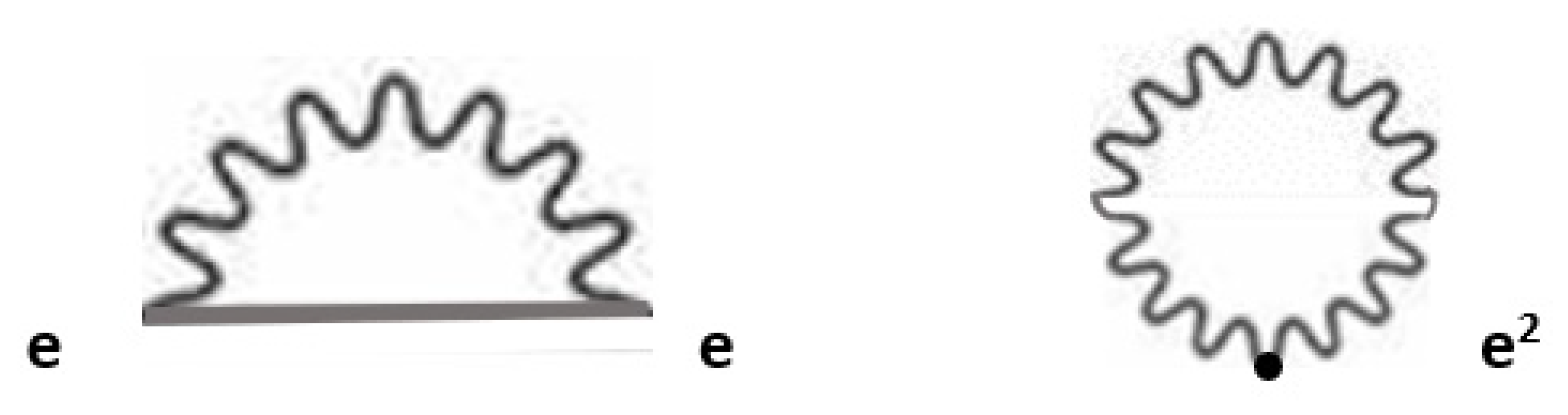
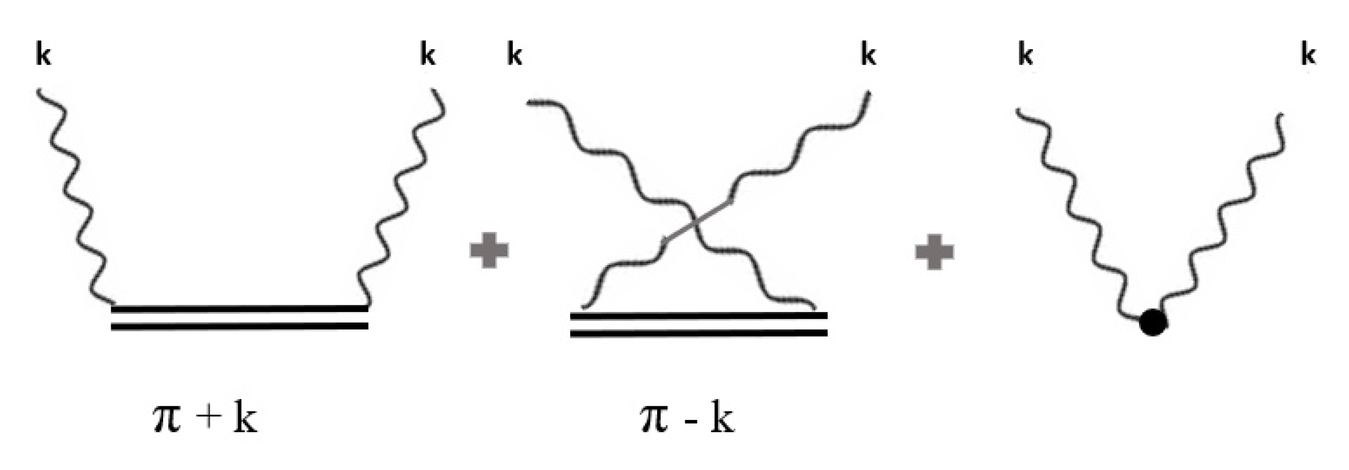
A discussed in Section 2, the space-time methods of Feynman, which were developed right after Bethe’s calculation, were helpful to provide a physical picture of the phenomena and facilitated calculations [38]. In that spirit, we consider the diagrams in Figure 1 that show to the order $e^2$ or $\alpha$ in the meson’s radiation field (one radiation field photon present) the processes that represent the $mas{s}^2$ operator $M_F^2$. By analyzing the $mas{s}^2$ operator in Section 4.3, we show these are indeed the appropriate Feynman diagrams.

In configuration space, the equation of motion for the free self-interacting meson is

$$\left(p^2+m_0^2\right)G_F\left(x^{\prime },x^{″}\right)+\int d^4{x}^{‴}{M}_F^2\left(x^{\prime }-x^{‴}\right)G_F\left(x^{‴},x^{″}\right)=\delta \left(x^{\prime }-x^{″}\right).$$

(36)

The presence of the convolution integral indicates we can view the meson as having a finite extent. The “shape” of the meson “centered” at $r^{\prime }$ is proportional the Fourier transform of $m_0^2+M_F^2\left(p\right)$, namely

$$\delta \left(r^{\prime }-r^{″}\right)+\frac{1}{m^2}\left(M_F^2\left(r^{\prime }-r^{″}\right)+m_0^2-m^2\right).$$

(37)

The effective finite extent of the meson in the vacuum field is central to the interpretation of the Lamb shift, as discussed in Section 2 and Section 3.3. Evidently, we can still say we have a point particle but now it is in a non-local potential. Although we need never explicitly mention the zero point vibrations in our field theoretic calculation we could interpret the Feynman diagrams as corresponding to the zero point fluctuations.

We can estimate the amplitude $\langle \overrightarrow{\xi }{}^2\rangle$ of the zero point oscillations (or equivalently the emission and absorption of virtual photons) by applying the uncertainty relations to the process depicted in Figure 1. When the photon is emitted, the particle receives a momentum $k_i$ with uncertainty $\Delta k_i$. Accordingly, the uncertainties in position $\overrightarrow{\xi }$ and velocity $\overrightarrow{v}$ of the particle satisfy the relations $\Delta \xi >1/\Delta k_i$ and $\Delta v_i\approx \Delta k_i/m$. Requiring that $\Delta v_i\approx 1$ implies that $\Delta k_i\approx m$ and $\Delta {\xi }_i>1/m=\mathrm{Compton}\mathrm{wavelength}$. To get the effective $\langle {\overrightarrow{\xi }}^2\rangle$, we must multiply by the probability that the photon has been emitted. The diagram has two vertices so the probability is proportional to $\alpha$, which leads to the result $\alpha {(\Delta \xi )}^2=\langle {\overrightarrow{\xi }}^2\rangle \approx 3\alpha /m^2$ the mean amplitude squared of the zero point vibrations, which is comparable to the result (Equation (28)) obtained using the equations of motion for the vector potential.

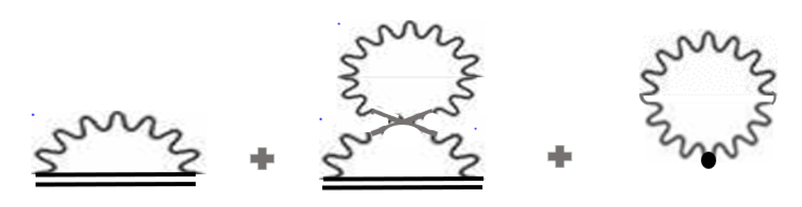
When we put a bare meson in an external potentia, we assume it forms a bound state. The propagator and therefore the equations of motion are as before except: (1) the free ${\left(mass\right)}^2$ operator $M_F^2$ is replaced by a bound state mass operator $M^2$; (2) the propagator $G_F$ for a free particle with radiative interaction is replaced by the corresponding propagator for a bound particle G; and (3) $p_{\mu }$ is replaced by the four-vector by ${\Pi }_{\mu }=p_{\mu }-V_{\mu }$, where $V_{\mu }$ is the external four-potential in accordance with minimal coupling [23]. The energy of the state is shifted by a mechanism similar to that for a free bare meson. The Feynman diagrams are shown in Figure 2.

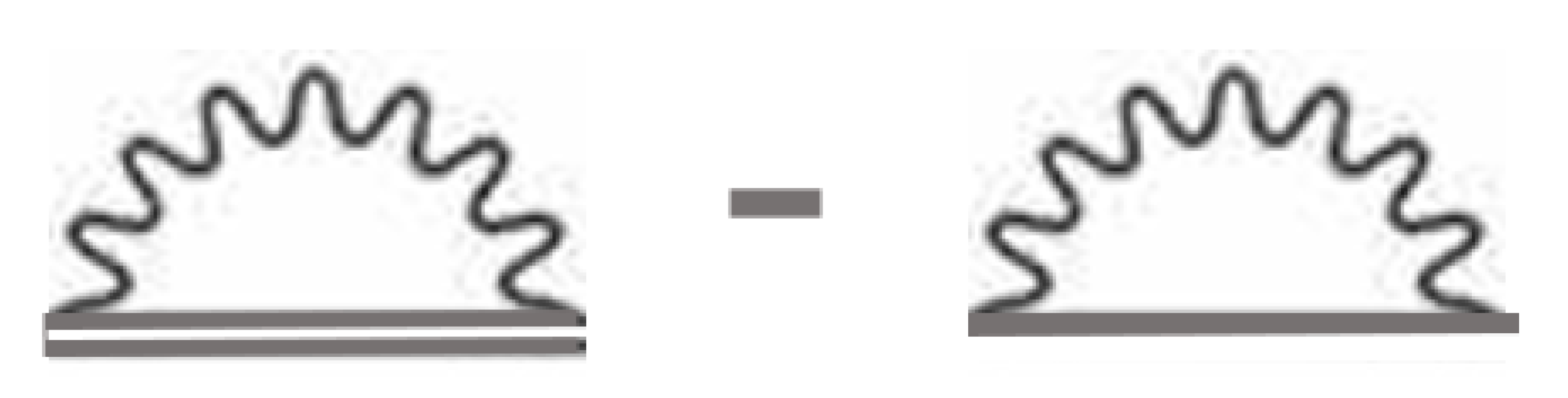
The double line represents a meson propagating in the external potential. The difference between the diagrams for the bound meson and the free meson is the radiative level shift (Figure 3). In other words, the radiative shift in a bound state level is the change in the self-energy of a particle that occurs when it becomes bound. As discussed in Section 2, this is exactly the way Bethe framed the problem of computing the Lamb shift. The intermediate state of the atom, i.e., while the virtual radiation field photon has been exchanged, is unknown. In his historic approach, the cumulative effect of these virtual transitions in given by the Bethe Log term.

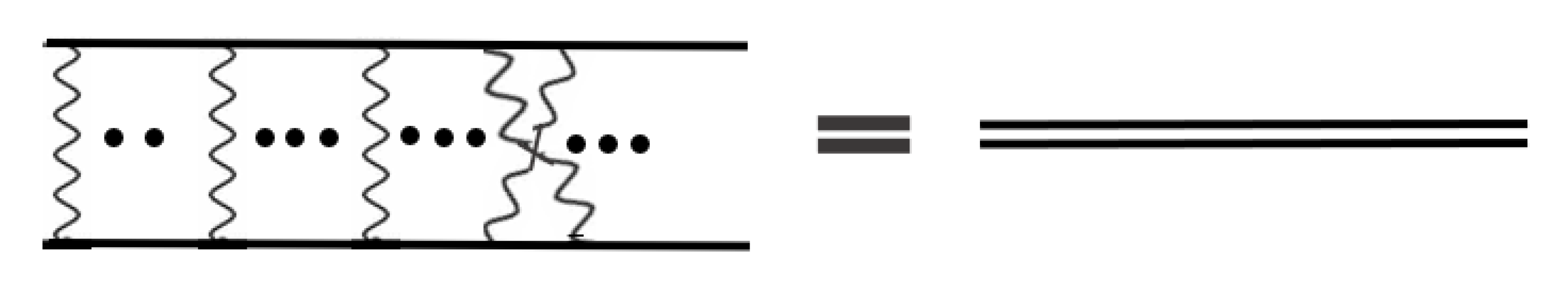
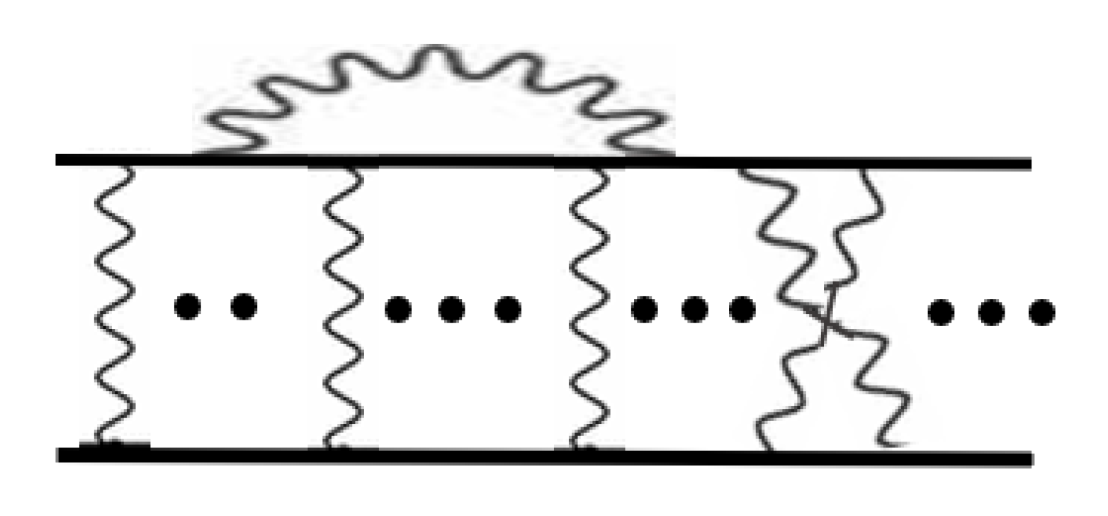
To indicate in more detail the process involved in the radiative shift for a Coulomb potential, we expand the double line representation of the bound meson, indicating separate meson and proton lines and the photons exchanged that represent the Coulomb force (Figure 4). The graphs giving the radiative shifts are of the form shown in Figure 5. The lowest-order shift, to order $\alpha$ (first order) in the radiation field and ${\left(Z\alpha \right)}^4$ (second order) in the Coulomb field, is given simply by the vertex correction (Figure 6).

Rather than consider separately all the various graphs in the Coulomb field and obtain an answer in a series with powers of $Z\alpha$ or $ln\left(Z\alpha \right)$ as is done with higher order calculations [7,51,67,72], we calculate the radiative correction using the equations of motion for a meson (spinless electron) in a Coulomb field and then make approximations to first order assuming that the proton or Coulomb source is an infinitely heavy point charge. We are neglecting recoil effects, center of mass corrections, radiative corrections and size effects for the proton. To include these effects we would use the Bethe–Salpeter equation [3,13,79]. On the other hand, Weinberg (in 1995) did not think the Bethe–Salpeter equation was the correct equation for relativistic interactions (it includes no crossed photon diagrams), and he concluded: "It must be said that the theory of relativistic effects and radiative corrections in bound states is not yet in entirely satisfactory shape [25]".

In general, we are concerned with directly measurable quantities, namely the shift in the difference between two energy levels of a bound meson. For example, we compute the change in the 2s − 2p separation. Clearly, this shift is given by the difference in renormalization between a meson bound in a 2s state and one bound in a 2p state. Thus, the renormalization of a free meson is never actually used.

4.2. Expressing the Radiative Shift in Terms of the Matrix Elements of the $Mas{s}^2$ Operator

From the equation for the propagator of a self- interacting meson in a potential $V^{\mu }\left(x\right)$, we find the equation obeyed by the corresponding meson wave functions. Taking mass renormalized wave functions of the meson in the potential field as our unperturbed states, we apply first-order perturbation theory to find the expression for the radiative shift in terms of matrix elements of the perturbation ${\overline{M}}^2$. The Green’s function or propagator for a meson field $\varphi \left(x^{\prime }\right)$ that interacts with its own radiation field and the external potential $V_{\mu }$ satisfies the equation:

$$\left({{\Pi }^{\prime }}^2+m^2+{\overline{M}}^2\right)G\left(x^{\prime },x^{″}\right)=\delta \left(x^{\prime }-x^{″}\right),$$

(38)

where

$${\Pi }_{\mu }^{\prime }=\frac{1}{i}{\partial }_{\mu }^{\prime }-V_{\mu }\left(x^{\prime }\right),$$

(39)

${\partial }_{\mu }^{\prime }=\partial /\partial x_{\mu }^{\prime }$ for $\mu =0,1,2,3$, and m is the physical mass. $M^2$ is the $mas{s}^2$ operator and ${\overline{M}}^2$ is the renormalized $mas{s}^2$ operator both for a meson in a Coulomb potential

$${\overline{M}}^2=M^2+m_0^2-m^2.$$

(40)

In Equation (38), we use a shorthand notation for the integration as in Equation (36). We assume our 4-potential is such that we can work in a gauge with $V_i=0,V^0=V\left(r\right)$. Since we want an energy shift, we take the Fourier transform of Equation (38) with respect to time

$$\left({p^{\prime }}^2-{(\overline{E}-V^{\prime })}^2+m^2+{\overline{M}}^2\left(\overline{E}\right)\right)G\left(\overline{E},{\overrightarrow{r}}^{\prime },{\overrightarrow{r}}^{″}\right)=\delta \left({\overrightarrow{r}}^{\prime }-{\overrightarrow{r}}^{″}\right),$$

(41)

where we define

$${\overline{M}}^2(\tilde{E})G\left(\tilde{E},{\overrightarrow{r}}^{\prime },{\overrightarrow{r}}^{″}\right)\equiv \int d^3{r}^{‴}{\overline{M}}^2\left(\tilde{E},{\overrightarrow{r}}^{\prime },{\overrightarrow{r}}^{‴}\right)G\left(\tilde{E},{\overrightarrow{r}}^{‴},{\overrightarrow{r}}^{″}\right),$$

(42)

and $\tilde{E}$ is the relativistic total energy. We can convert Equation (41) to an equation for the wave functions by expressing the Green’s function as the vacuum expectation value of the time ordered product, signified by a plus sign, of the meson field $\varphi \left(x^{\prime }\right)$ and its adjoint ${\varphi }^{†}\left(x^{″}\right)$:

$$G\left(x^{\prime },x^{″}\right)=i〈{\left(\varphi \left(x^{\prime }\right){\varphi }^{†}\left(x^{″}\right)\right)}_{+}〉.$$

(43)

If we insert a complete set of eigenstates of the Hamiltonian (particle, antiparticle, bound, and scattering) in this equation for G and use the equation of motion for $\varphi \left(x\right)$:

$$\varphi (\overrightarrow{r},t)=e^{iHt}\varphi (\overrightarrow{r},0)e^{-iHt},$$

(44)

we find

$$G\left(\tilde{E},{\overrightarrow{r}}^{\prime },{\overrightarrow{r}}^{″}\right)=\sum _m\frac{{\mathsf{\Phi }}_m\left({\overrightarrow{r}}^{\prime }\right){\mathsf{\Phi }}_m\left({\overrightarrow{r}}^{″}\right)}{\tilde{E}-{\tilde{E}}_m}+\mathrm{contributions}\mathrm{scattering}\mathrm{states}.$$

(45)

The ${\mathsf{\Phi }}_m\left(\overrightarrow{r}\right)$ are the relativistic bound state particle wave functions $\langle 0|\varphi (\overrightarrow{r},0)|{\tilde{E}}_m\rangle$ with the renormalized mass and a relativistic total energy ${\tilde{E}}_m$. If Equation (41) is to be satisfied when we substitute this form for G and let $m=n$, $\tilde{E}={\tilde{E}}_n$, and $r^{\prime }\ne r^{″}$, then it follows that

$$\left({p^{\prime }}^2+m^2-{\left({\tilde{E}}_n-V^{\prime }\right)}^2+{\overline{M}}^2\left({\tilde{E}}_n\right)\right){\mathsf{\Phi }}_n\left({\overrightarrow{r}}^{\prime }\right)=0.$$

(46)

We now use first order perturbation theory to calculate the radiative shift due to ${\overline{M}}^2({\tilde{E}}_n)$. The unperturbed wave functions are the renormalized relativistic wave functions ${\tilde{\psi }}_n\left(\overrightarrow{r}{}^{\prime }\right)$ for a meson which satisfy the equation

$$\left[{p^{\prime }}^2-{({\tilde{E}}_n^0-V^{\prime })}^2+m^2\right]{\tilde{\psi }}_n\left(\overrightarrow{r}{}^{\prime }\right)=0,$$

(47)

where ${\tilde{E}}_n^0$ is the unperturbed relativistic energy eigenvalue. For our normalization, we choose

$$\left({\tilde{\psi }}_n,\left({\tilde{E}}_n^0-V\right){\widehat{\psi }}_n\right)=m,$$

(48)

where the scalar product is defined as follows:

$$(\varphi ,A\psi )=\int d^3{r}^{\prime }{\varphi }^{*}\left({\overrightarrow{r}}^{\prime }\right)\left(A\psi \left({\overrightarrow{r}}^{\prime }\right)\right).$$

(49)

We take the scalar product of Equation (46) with ${\tilde{\psi }}_n$ and substitute Equations (48) and (49) to obtain, in lowest order in the radiation field, the shift for the state N:

$$\Delta {\tilde{E}}_N\equiv {\tilde{E}}_N-{\tilde{E}}_N^0=\frac{1}{2m}({\tilde{\psi }}_N,{\overline{M}}^2({\tilde{E}}_N){\tilde{\psi }}_N),$$

(50)

which is shorthand for

$$\Delta {\tilde{E}}_N=\frac{1}{2m}\int d^{3}r{\tilde{\psi }}_N^{*}\left({\overrightarrow{r}}^{\prime }\right)\int d^3{r}^{″}{\overline{M}}^2\left({\tilde{E}}_N,{\overrightarrow{r}}^{\prime },{\overrightarrow{r}}^{″}\right){\tilde{\psi }}_N\left({\overrightarrow{r}}^{″}\right).$$

(51)

If we define the relativistic state $|\tilde{n}\rangle$ such that ${\tilde{\psi }}_n({\overrightarrow{r}}^{\prime })\equiv \langle r^{\prime }|\tilde{n}\rangle$ and note that

$${\overline{M}}^2\left({\tilde{E}}_n,{\overrightarrow{r}}^{\prime },{\overrightarrow{r}}^{″}\right)=〈r^{\prime }\left|{\overline{M}}^2({\tilde{E}}_n)\right|r^{″}〉,$$

(52)

then we obtain the simple and important result

$$\Delta {\tilde{E}}_N=\frac{1}{2m}〈\tilde{N}\left|{\overline{M}}^2\left({\tilde{E}}_N\right)\right|\tilde{N}〉.$$

(53)

The radiative shift of the level ${\tilde{E}}_N$ equals $1/2m$ times the expectation value of the renormalized $mas{s}^2$ operator ${\overline{M}}^2({\tilde{E}}_N)$ with respect to the state $\langle \tilde{N}|$, where $\tilde{E}$ is the relativistic energy.

In Section 4.3, we derive an expression for ${\overline{M}}^2$ to order $\alpha$ in the radiation field by using the equations of motion for the meson in an external potential, a method we believe is closest to fundamental principles.

S Matrix Approach

As an alternative to our approach, we should mention that it is possible to use the S matrix formalism to find the radiative shift. As mentioned in Section 2, Dyson showed the equivalence of the formulations of QED of Schwinger and Feynman with the S matrix formalism [47,48]. For the interaction Lagrangian, we use

$$L_{\mathrm{int}}={ej}_{\mu }{A}_{\mathrm{rad}}^{\mu },$$

(54)

where $A_{\mathrm{rad}}^{\mu }$ is the meson’s radiation field and $j^{\mu }$ is the meson current in the potential field. We calculate the S matrix element between pure bound states with the usual harmonic time dependence. Since we have a perturbation to a bound state the matrix element must be expressible in the form ${\langle S\rangle }_N=e^{-iT\left({\tilde{E}}_N-{\tilde{E}}_N^0\right)}$ where T is the interaction time. To obtain the shift we perform the integrations and use the usual trick of equating T and $2\pi \delta \left(0\right)$.

4.3. Derivation of $Mas{s}^2$ Operator for Relativistic Meson (Spinless Electron) in an External Potential

We now outline the calculation of ${\overline{M}}^2(\tilde{E})$ in a covariant gauge in which the meson’s radiation field $A_{\mathrm{rad}}^{\mu }$ and the meson field $\varphi$ obey the equations:

$$\begin{array}{cc}\hfill {\left[A_{\mathrm{rad}}^{\mu }\left(x^{\prime }\right),A_{\mathrm{rad}}^{\nu }\left(x^{″}\right)\right]}_{t^{\prime }=t^{″}}& =i{g}^{\mu \nu }\delta x^{\prime }-x^{″},\hfill \\ \hfill \left[A_{\mathrm{rad}}^0(\overrightarrow{r}{}^{\prime },t),\varphi (\overrightarrow{r}{}^{″},t)\right]& =0,\hfill \\ \hfill \left[{\partial }_0{A}_{\mathrm{rad}}^0(\overrightarrow{r}{}^{\prime },t),\varphi (\overrightarrow{r}{}^{″},t)\right]& =0.\hfill \end{array}$$

(55)

Since the results are gauge invariant, we can choose the Feynman gauge in order to simplify the calculation. In the final answer, we simply replace the Feynman propagator with the radiation gauge propagator. The derivation proceeds by converting the Klein–Gordon equation for a self-inter-acting meson in an external potential into an equation for the corresponding Green’s function $G(x^{\prime },x^{″})$. An explicit form for $M^2(\tilde{E})$ is then obtained by comparing this equation to the defining equation for G which includes $M^2$ (Equation (38)). If desired, one may skip to Section 4.3.2.

4.3.1. Detailed Derivation of $Mas{s}^2$ Operator from Equations of Motion

To take electromagnetic self-interactions into account in the Klein–Gordon equation, we make the substitution

$${\Pi }_{\mu }^{\prime }\to {\Pi }_{\mu }^{\prime }-e{A}_{\mu ,\mathrm{rad}}\left(x^{\prime }\right).$$

(56)

${\Pi }_{\mu }^{\prime }$ is defined in Equation (39)) with the result

$$({{\Pi }^{\prime }}^2+m_0^2)\varphi \left(x^{\prime }\right)=j\left(x^{\prime }\right),$$

(57)

where

$$j\left(x^{\prime }\right)=e\left\{A_{\mu }^{\mathrm{rad}}\left(x^{\prime }\right),{{\Pi }^{\prime }}^{\mu }\right\}\varphi \left(x^{\prime }\right)-e^2{A}_{\mathrm{rad}}^{\mu }\left(x^{\prime }\right)A_{\mu ,\mathrm{rad}}\left(x^{\prime }\right)\varphi \left(x^{\prime }\right).$$

(58)

The anticommutator insures that the $A·p$ term is Hermitean. To convert Equation (57) into an equation for $G(x^{\prime },x^{″})$, we make use of Equation (43). We multiply by ${\varphi }^{†}\left(x^{″}\right)$, time order, and take the vacuum expectation value. We use the equation

$$\begin{array}{cc}\hfill {{\partial }^{\prime }}^2{\left(A\left(x^{\prime }\right)B\left(x^{″}\right)\right)}_{+}& ={\left({{\partial }^{\prime }}^{2}A\left(x^{\prime }\right)B\left(x^{″}\right)\right)}_{+}\hfill \\ & +\left[{{\partial }_0}^{\prime }A\left(x^{\prime }\right),B\left(x^{″}\right)\right]\delta \left(t^{\prime }-t^{″}\right)\hfill \\ & +{{\partial }_0}^{\prime }\left[A\left(x^{\prime }\right),B\left(x^{″}\right)\right]\delta \left(t^{\prime }-t^{″}\right)\hfill \\ & +\left[A\left(x^{\prime }\right),B\left(x^{″}\right)\right]{\delta }^{\prime }\left(t^{\prime }-t^{″}\right),\hfill \end{array}$$

(59)

which follows from the lemma

$${{\partial }_0}^{\prime }{\left(A\left(x^{\prime }\right)B\left(x^{″}\right)\right)}_{+}={\left({\partial }_{0}A\left(x^{\prime }\right)B\left(x^{″}\right)\right)}_{+}+\left[A\left(x^{\prime }\right),B\left(x^{″}\right)\right]\delta \left(t^{\prime }-t^{″}\right),$$

(60)

to obtain the result

$$\left({{\Pi }^{\prime }}^2+m_0^2\right)G\left(x^{\prime },x^{″}\right)=+\delta \left(x^{\prime }-x^{″}\right)+i〈{\left(j\left(x^{\prime }\right){\varphi }^{†}\left(x^{″}\right)\right)}_{+}〉.$$

(61)

Since we are calculating ${\overline{M}}^2$ to order $e^2$ in the radiation field the term $e^2\langle (A_{\mu }^{\mathrm{rad}}{\left(x^{\prime }\right)}_{\mathrm{rad}}^{\mu }\left(x^{\prime }\right)\varphi \left(x^{\prime }\right){\varphi }^{†}{\left(x^{″})\right)}_{+}\rangle$ in $\langle {(j(x^{\prime }){\varphi }^{†}(x^{″}))}_{+}\rangle$ may be calculated with a free photon field rather than the radiation field. In essence this follows since the radiation field is equal to the free field plus terms of higher order. To show the formal justification, consider the matrix element

$$\sigma =\langle {\left(A^{\mu }\left({\xi }^{\prime }\right)A^{\nu }\left({\xi }^{″}\right)\varphi \left(x^{\prime }\right){\varphi }^{†}\left(x^{″}\right)\right)}_{+}\rangle .$$

(62)

where ${\xi }^{\prime }$ is a four-vector that the vector potential depends on [112]. Recall

$${\partial }_{{\xi }^{\prime }}^2{A}^{\mu }\left({\xi }^{\prime }\right)=e{j}^{\mu }\left(\xi {}^{\prime }\right),$$

(63)

where thus

$$\begin{array}{cc}\hfill {\partial }_{\xi {}^{\prime }}{}^2\sigma & =e〈{\left(j^{\mu }\left({\xi }^{\prime }\right)A^{\nu }\left({\xi }^{″}\right)\varphi \left(x^{\prime }\right){\varphi }^{†}\left(x^{″}\right)\right)}_{+}〉\hfill \\ & \left.+i{g}^{\mu \nu }\delta \left({\xi }^{\prime }\right.-{\xi }^{″}\right)〈{\left(\varphi \left(x^{\prime }\right){\varphi }^{†}\left(x^{″}\right)\right)}_{+}〉.\hfill \end{array}$$

(64)

To lowest order, we may drop the first term. Solving for $\sigma$ gives

$$\sigma =\left[g^{\mu \nu }\frac{1}{{\partial }_{\xi \prime }{}^2}\delta \left({\xi }^{\prime }-{\xi }^{″}\right)\right]G\left(x^{\prime },x^{″}\right).$$

(65)

Considering the boundary conditions, we realize the term in brackets is just the usual Feynman propagator. Accordingly, we obtain

$$\sigma =-D^{\mu \nu }\left({\xi }^{\prime }-{\xi }^{″}\right)G\left(x^{\prime },x^{″}\right).$$

(66)

This result is to be expected since to lowest order the complete Hilbert space factors into two independent spaces, one for $\varphi \left(x^{\prime }\right)$ and one for $A\left(x^{\prime }\right)$. Thus, we show that

$$\begin{array}{cc}\hfill 〈{\left(j\left(x^{\prime }\right)\varphi \left(x^{″}\right)\right)}_{+}〉& =i{e}^2〈{\left(A_{\mu }\left(x^{\prime }\right)A^{\mu }\left(x^{\prime }\right)\right)}_{+}〉G\left(x^{\prime },x^{″}\right)\hfill \\ & +e〈{\left(\left(A_{\mu }^{\mathrm{rad}}\left(x^{\prime }\right){{\Pi }^{\prime }}^{\mu }+{{\Pi }^{\prime }}^{\mu }{A}_{\mu }^{\mathrm{rad}}\left(x^{\prime }\right)\right)\varphi \left(x^{\prime }\right)\varphi \left(x^{″}\right)\right)}_{+}〉.\hfill \end{array}$$

(67)

We can rewrite the second term on the right side using the notation

$$\begin{array}{c}\hfill {{\overrightarrow{\Pi }}^{\prime }}^{\mu }{A}_{\mu }^{\mathrm{rad}}\left(x^{\prime }\right)\varphi \left(x^{\prime }\right)\equiv \left(A_{\mu }^{\mathrm{rad}}\left(x^{\prime }\right){{\Pi }^{\prime }}^{\mu }+{{\Pi }^{\prime }}^{\mu }{A}_{\mu }^{\mathrm{rad}}\left(x^{\prime }\right)\right)\varphi \left(x^{\prime }\right)\\ \hfill =\left(\frac{1}{i}{\partial }_{\xi {}^{\prime }}^{\mu }+\frac{2}{i}{\partial }_{x^{\prime }}^{\mu }-2V^{\mu }\left(x^{\prime }\right)\right)A_{\mu }^{\mathrm{rad}}\left({\xi }^{\prime }\right)\varphi {\left(x^{\prime }\right)}_{{\xi }^{\prime }=x^{\prime }}.\end{array}$$

(68)

From Equation (61), we have

$$\begin{array}{cc}\hfill \left({{\Pi }^{\prime }}^2+m_0^2\right)G\left(x^{\prime },x^{″}\right)& =\delta \left(x^{\prime }-x^{″}\right)+ie{{\overrightarrow{\Pi }}^{\prime }}^{\mu }\langle {\left(A_{\mu }^{\mathrm{rad}}\left(x^{\prime }\right)\varphi \left(x^{\prime }\right){\varphi }^{†}\left(x^{″}\right)\right)}_{+}〉\hfill \\ & -e^2〈{\left(A_{\mu }\left(x^{\prime }\right)A^{\mu }\left(x^{\prime }\right)\right)}_{+}〉G\left(x^{\prime },x^{″}\right).\hfill \end{array}$$

(69)

Using Equations (38) and (40) for the unrenormalized $mas{s}^2$ operator $M^2$ shows the last two terms on the right side of Equation (69) are equal to

$$-M^{2}G(x^{\prime },x^{″})=ie{{\overrightarrow{\Pi }}^{\prime }}^{\mu }\langle {\left(A_{\mu }^{\mathrm{rad}}\left(x^{\prime }\right)\varphi \left(x^{\prime }\right){\varphi }^{†}\left(x^{″}\right)\right)}_{+}\rangle -e^2〈{\left(A_{\mu }\left(x^{\prime }\right)A^{\mu }\left(x^{\prime }\right)\right)}_{+}〉G\left(x^{\prime },x^{″}\right).$$

(70)

where $M^{2}G(x^{\prime },x^{″})$ represent a convolution integral as in Equation (42). To order $e^2$, we may replace the full propagator G by the propagator $G^c$ for a particle in the potential with the physical mass:

$$\left({{\Pi }^{\prime }}^2+m^2\right)G^C\left(x^{\prime },x^{″}\right)=\delta \left(x^{\prime }-x^{″}\right).$$

(71)

Operating on Equation (70) from the right with ${\Pi }^2\left(x^{″}\right)+m^2$ therefore gives

$$\begin{array}{cc}\hfill M^2\left(x^{\prime },x^{″}\right)& =-ie{{\overrightarrow{\Pi }}^{\prime }}^{\mu }\langle {\left(A_{\mu }^{\mathrm{rad}}\left(x^{\prime }\right)\varphi \left(x^{\prime }\right){\varphi }^{†}\left(x^{″}\right)\right)}_{+}\rangle \left({\Pi }^2\left(x^{″}\right)+m^2\right)\hfill \\ & +e^2〈{\left(A_{\mu }\left(x^{\prime }\right)A^{\mu }\left(x^{\prime }\right)\right)}_{+}〉\delta \left(x^{\prime }-x^{″}\right).\hfill \end{array}$$

(72)

Following the same procedure as before gives the result

$$\begin{array}{cc}\hfill M^2\left(x^{\prime },x^{″}\right)=-i{e}^2& \overrightarrow{{\Pi }^{\mu }}\left(x^{\prime }\right)〈{\left(A_{\mu }\left(x^{\prime }\right)A^{\nu }\left(x^{″}\right)\varphi \left(x^{\prime }\right){\varphi }^{†}\left(x^{″}\right)\right)}_{+}〉\overleftarrow{{\Pi }_{\nu }}\left(x^{″}\right)\hfill \\ & +e^2〈{\left(A_{\mu }\left(x^{\prime }\right)A^{\mu }\left(x^{\prime }\right)\right)}_{+}〉\delta \left(x^{\prime }-x^{″}\right),\hfill \end{array}$$

(73)

which is a shorthand notation for

$$\begin{array}{cc}\hfill M^2\left(x^{\prime },x^{″}\right)=i{e}^2& \left(\frac{2}{i}{\partial }_{x^{\prime }}^{\mu }+\frac{1}{i}{\partial }_{{\xi }^{\prime }}^{\mu }-2V^{\mu }\left(x^{\prime }\right)\right)D_{\mu \nu }\left({\xi }^{\prime }-{\xi }^{″}\right)G^c\left(x^{\prime },x^{″}\right)\times \hfill \\ & \left(\frac{2}{i}{\partial }_{x^{″}}^{\nu }+\frac{1}{i}{\partial }_{{\xi }^{″}}^{\nu }-2V^{\mu }\left(x^{″}\right)\right){|}_{{\xi }^{″}=x^{″},{\xi }^{\prime }=x^{\prime }}-i{e}^2{D}_{\mu }^{\mu }\left(0\right)\delta (x^{\prime }-x^{″}).\hfill \end{array}$$

(74)

Since our calculation is to order $e^2$, we again substitute $G^c$ for $G(x^{\prime },x^{″})$. Now that we have derived the equation for $M^2(x^{\prime },x^{″})$, we return to the radiation gauge.

4.3.2. The Expression for $M^2(\tilde{E})$

For our calculation of the radiative shift, we need the operator corresponding to the time Fourier transform of $M^2(x^{\prime },x^{″})$. To obtain this result, we use the expression for $G^c$ which follows from Equation (71) and time translation invariance [113]:

$$G^c\left(x^{\prime },x^{″}\right)={\int }_{-\infty }^{\infty }\frac{d\tilde{E}}{2\pi }〈r^{\prime }\left|\frac{1}{{\Pi }^2+m^2-iϵ}\right|r^{″}〉e^{-i\tilde{E}(t^{\prime }-t^{″})},$$

(75)

where

$$\begin{array}{ccc}\hfill {\Pi }^k& =p^k,\hfill & \hfill {\Pi }^0=\tilde{E}-V\left(r\right).\end{array}$$

(76)

If we substitute Equation (75) and

$$D_{\mu \nu }\left({\xi }^{\prime }-{\xi }^{″}\right)=\int \frac{d^{4}k}{{\left(2\pi \right)}^4}{e}^{ik\left({\xi }^{\prime }-{\xi }^{″}\right)}{D}_{\mu \nu }\left(k\right),$$

(77)

into our expression for $M^2$, Equation (74), and we note the derivative with respect to ${\xi }_{\mu }^{\prime }$ brings down a factor of $k_{\mu }$, we find, after some computation, the important result for the unrenormalized relativistic $mas{s}^2$ operator

$$M^2(\tilde{E})=\frac{i{e}^2}{2}\int \frac{d^{4}k}{{\left(2\pi \right)}^4}{D}_{\mu \nu }\left(k\right)T^{\mu \nu },$$

(78)

where

$$\begin{array}{cc}\hfill T^{\mu \nu }& =\left(2{\Pi }^{\mu }-k^{\mu }\right)\frac{1}{{(\Pi -k)}^2+m^2}\left(2{\Pi }^{\nu }-k^{\nu }\right)\hfill \\ & +\left(2{\Pi }^{\nu }+k^{\nu }\right)\frac{1}{{(\Pi +k)}^2+m^2}\left(2{\Pi }^{\mu }+k^{\mu }\right)-2g^{\mu \nu }.\hfill \end{array}$$

(79)

We exploit the symmetry of the photon propagator under $k\to -k$ to write $T^{\mu \nu }$ in a form that manifests crossing symmetry. From the Feynman rules we see that the diagrams corresponding to the $T^{\mu \nu }$ operator are as shown in Figure 7.

The double line in the figure refers to the meson propagating in an external potential. $T^{\mu \nu }$ is the operator Compton scattering amplitude in the forward direction. The seagull term on the right in Figure 7 must be included to insure gauge invariance. At threshold, it gives the Thomson scattering amplitude. As Equation (78) indicates, we obtain the diagrams for $M^2$ by contracting the above diagrams for $T^{\mu \nu }$ with the diagram for the photon propagator $D_{\mu \nu }$, giving the resulting Feynman diagrams for $M^2$ in Figure 8. The crossed diagram may be deformed into the uncrossed diagram, therefore both diagrams give equal contributions to $M^2$. Note that, in a calculation of the shift between two levels, the bubble term gives no contribution since its matrix elements are independent of the state.

4.3.3. Gauge Invariance of the Shift $\Delta \widetilde{E_N}$ for a Relativistic Meson (Spinless Electron)

We must show that the most general gauge transformation [26]

$$D_{\mu \nu }\to D_{\mu \nu }+{\lambda }^{\prime }{n}_{\mu }{k}_{\nu }+{\mu }^{\prime }{n}_{\nu }{k}_{\mu }+{\nu }^{\prime }{k}_{\mu }{k}_{\nu },$$

(80)

induces no change in the observed shift. Under a gauge transformation, the radiative shift changes by an amount

$$\delta \left(\Delta {\tilde{E}}_N\right)=\frac{1}{2m}\frac{i{e}^2}{2}\int \frac{d^{4}k}{{\left(2\pi \right)}^4}〈\tilde{N}\left|{\lambda }^{\prime }{n}_{\mu }{k}_{\nu }{T}^{\mu \nu }+{\mu }^{\prime }{n}_{\nu }{k}_{\mu }{T}^{\mu \nu }++{\nu }^{\prime }{k}_{\mu }{k}_{\nu }{T}^{\mu \nu }\tilde{N}\right|〉.$$

(81)

We contract $T^{\mu \nu }$ with $k_{\mu }$ and use the identities

$$\begin{array}{c}k(2\Pi +k)={(\Pi +k)}^2+m^2-\left({\Pi }^2+m^2\right)\hfill \\ k(2\Pi -k)=-[{(\Pi -k)}^2+m^2]+{\Pi }^2+m^2\hfill \end{array},$$

(82)

to obtain

$$\begin{array}{cc}\hfill k_{\mu }{T}^{\mu \nu }& =\left(2{\Pi }^{\nu }+k^{\nu }\right)-\left({\Pi }^2+m^2\right)\frac{1}{{(\Pi +k)}^2+m^2}\left(2{\Pi }^{\nu }+k^{\nu }\right)\hfill \\ & -\left(2{\Pi }^{\nu }-k^{\nu }\right)+\left(2{\Pi }^{\nu }-k^{\nu }\right)\frac{1}{{(\Pi -k)}^2+m^2}\left({\Pi }^2+m^2\right)\hfill \\ & -2k^{\nu }.\hfill \end{array}$$

(83)

For our unperturbed basis states, we have

$$\left({\Pi }^2+m^2\right)|\tilde{N}\rangle =0.$$

(84)

Consequently, $\langle \tilde{N}\left|k_{\mu }{T}^{\mu \nu }\right|\tilde{N}\rangle =0$ and since $T^{\mu \nu }\left(k\right)=T^{\nu \mu }(-k)$ it follows that $\langle \tilde{N}\left|k_{\nu }{T}^{\mu \nu }\right|\tilde{N}\rangle =0,$ Accordingly, we see that $T^{\mu \nu }$ is gauge invariant between physical states and that $\delta (\Delta \widetilde{E_N})$ vanishes.

5. Calculation of the Radiative Shifts in the Nonrelativistic Approximation

5.1. Relationship to the Dipole Approximation

The dipole approximation and the nonrelativistic approximation are often considered as two separate approximations. In radiative shift calculations, the dipole approximation is often given by the prescription: in the radiation gauge, compute the shift ignoring the dependence of $T^{\mu \nu }$ on the photon three-momentum $\overrightarrow{k}$. As a consequence, we find that the term $T^{00}{g}_{00}$ corresponding to the static Coulomb or longitudinal photon interaction gives a vanishing contribution to the shift. Seen in this way the dipole approximation breaks gauge invariance which is why we must specify the gauge.

Another form of the dipole approximation is to let $\overrightarrow{A}\left(\overrightarrow{r}\right)$ be independent of $\overrightarrow{r}$. To understand the properties of this form of the dipole approximation under gauge transformations consider the nonrelativistic interaction Hamiltonian for radiation with a four-potential $(\varphi \left(\overrightarrow{r}\right),\overrightarrow{A}\left(\overrightarrow{r}\right))$ and a scalar particle of charge e and mass m:

$$H_I=-\frac{e}{m}(\overrightarrow{p}·\overrightarrow{A})+e\varphi .$$

(85)

Under a gauge transformation $\overrightarrow{A}\to \overrightarrow{A}+\overrightarrow{\nabla }\lambda$, $\varphi \to \varphi -{\partial }_t\lambda$, and $H_I$ transforms into $H_I+\mathsf{\Lambda }$, where

$$\mathsf{\Lambda }=-\frac{e}{m}\overrightarrow{p}·\overrightarrow{\nabla }\lambda -e{\partial }_t\lambda .$$

(86)

To obtain gauge invariance, the matrix elements of between the initial and final states must vanish: $\langle f\left|\mathsf{\Lambda }\right|i\rangle =0$. If we let $\lambda =e^{i\overrightarrow{k}·\overrightarrow{r}-i\omega t}$, then gauge invariance requires that

$$\langle f|\frac{1}{m}\overrightarrow{p}·\overrightarrow{k}{e}^{i\overrightarrow{k}·\overrightarrow{r}}-\omega e^{i\overrightarrow{k}·\overrightarrow{r}}|i\rangle =0.$$

(87)

Following the customary prescription for the dipole approximation, we set $exp(i\overrightarrow{k}·\overrightarrow{r})$ equal to unity, then, since $\langle f|i\rangle =0$, we conclude that the matrix element $\langle f|\overrightarrow{p}·\overrightarrow{k}|i\rangle$ must vanish if we are to obtain gauge invariance. Clearly, this is not generally the case and gauge invariance is violated. The difficulty lies in the fact that setting the exponential equal to one resulted in approximating the change in the vector potential to first order in k and the change in the scalar potential to zero order in k. If we approximate the change in the scalar potential to one order higher, then we find that gauge invariance requires

$$\langle f|\frac{1}{m}\overrightarrow{p}·\overrightarrow{k}-i\omega \overrightarrow{k}·\overrightarrow{r}|i\rangle =0.$$

(88)

This quantity does indeed vanish since

$$\begin{array}{cc}\hfill 〈f\left|\frac{\overrightarrow{p}}{m}\right|i〉& =i\langle f|[H,\overrightarrow{r}]\rangle i\rangle =i\left(E_f-E_i\right)\langle f|\overrightarrow{r}|i\rangle \hfill \\ & =i\omega \langle f\left|\overrightarrow{r}\right|i\rangle .\hfill \end{array}$$

(89)

In the radiation gauge, the scalar potential vanishes, thus we circumvent these difficulties.

Alternatively, we may obtain the unrenormalized $M^2$ operator in the nonrelativistic approximation from a different perspective, by noting that the pole in the photon propagator in Equation (78) insures that the integration over $k^0$ leads to the result $|\overrightarrow{k}|=k^0$ but since $|\overrightarrow{k}|$ is a momentum it equals a frequency over the speed of light $|\overrightarrow{k}|=\omega /c,$ As c increases the magnitude of the spatial momentum vanishes and we obtain the dipole approximation. Seen in this way, the dipole approximation is not gauge dependent but simply part of the nonrelativistic approximation. If we work in the radiation gauge, then this method gives the result obtained from the usual proscription.

From dynamical considerations we can show that in a bound system characterized by a small coupling constant the motion is nonrelativistic and $|\overrightarrow{k}|$, the approximate change in momentum for radiative transitions between states, may be neglected with respect to the momentum p of the bound particle.

Consider a potential of the form

$$V\left(r\right)=\frac{1}{n}m{g}^{n+2}{\left(mr\right)}^n,n>-2.$$

(90)

The exponent of the mass m is chosen so that the coupling constant g is dimensionless; the exponent of g and the overall coefficient are chosen so that V agrees with the conventional expressions for the simple harmonic oscillator $(n=2,g=\sqrt{{\omega }_0/m}$ and the Coulomb potential $(n=-1,g=Z\alpha )$. The total nonrelativistic energy of the atom is $E=T+V$. Employing the virial theorem for our potential $\overline{T}=-(n/2)\overline{V}$ and the uncertainty principle gives the results

$$\begin{array}{cccc}\hfill p& \approx \frac{1}{r}\approx gmc,\hfill & \hfill E& \approx \frac{n+2}{2n}{g}^{2}m{c}^2,\hfill \end{array}$$

(91)

where c is the speed of light. These results justify the use of nonrelativistic dynamics for small g. The contribution to the shift of a bound state energy level will be greatest for resonant virtual transitions, that is, when the photon energy equals the difference between two energy levels. For these resonant transitions $E\approx |\overrightarrow{k}|c$ and

$$\left|\overrightarrow{\frac{k}{p}}\right|\sim \left|\frac{n+2}{2n}\right|g<<1,$$

(92)

for weak coupling. To insure that the nonrelativistic approximations remain valid during the integration over frequency, it may be necessary to use a cut off which is proportional to the mass. The shift for greater (and therefore nonresonant) frequencies for physically realistic situations can be calculated by neglecting the bound state energy and keeping only the lowest order terms in the coupling constant.

To understand the physical meaning of the dipole approximation more clearly, we employ the translation operator in momentum space $e^{i\overrightarrow{k}·\overrightarrow{r}}$ to show that for a function $f\left(p\right)$ we have the identity

$$\langle N|(2\overrightarrow{p}-\overrightarrow{k})f(\overrightarrow{p}-\overrightarrow{k})(2\overrightarrow{p}-\overrightarrow{k})|N\rangle =(\langle N|e^{i\overrightarrow{k}·\overrightarrow{r}})(2\overrightarrow{p}+\overrightarrow{k})f(\overrightarrow{p})(2\overrightarrow{p}+\overrightarrow{k})(e^{-i\overrightarrow{k}·\overrightarrow{r}}|N\rangle ).$$

(93)

Applying this result to the expressions for $M^2\left(E\right)$ and $T^{\mu \nu }$ (Equations (78) and (79)), we see that the matrix elements for the shift are between translated atomic states $(e^{-i\overrightarrow{k}·\overrightarrow{r}}|N\rangle )$ that have a center of mass momentum $-\overrightarrow{k}$ in order to conserve momentum when the virtual photon of momentum $+\overrightarrow{k}$ is emitted. In addition, from the Feynman rules for spinless mesons, we know that the $\overrightarrow{k}$ present in $2\overrightarrow{p}+\overrightarrow{k}$ insures momentum conservation at the vertex. Accordingly dropping the $\overrightarrow{k}$ dependence means that we are violating momentum conservation and neglecting the recoil of the particle, which is a reasonable approximation since we are dealing with long wavelength photons whose momentum is much less than the particle’s momentum. In more accurate calculations, we need to maintain center of mass momentum conservation and include the corresponding recoil terms [3,7,51,67,72,87].

5.2. $M^2$ in the Nonrelativistic Dipole Approximation

We first take the nonrelativistic limit of our expression for $T^{\mu \nu }$ (Equation (79)). We obtain the crossing symmetric, gauge invariant Compton scattering amplitude operator in the forward direction for a meson or a spinless Schrodinger electron in a potential V:

$$\begin{array}{cc}\hfill T^{ij}& =\left(2p_i-k_i\right)\frac{1}{{(\overrightarrow{p}-\overrightarrow{k})}^2+2mV-\left(E-k^0\right)2m}\left(2p_j-k_j\right)\hfill \\ & +\left(2p_j+k_j\right)\frac{1}{{(\overrightarrow{p}+\overrightarrow{k})}^2+2mV-\left(E+k^0\right)2m}\left(2p_i+k_i\right)-2g^{ij},\hfill \end{array}$$

(94)

$$\begin{array}{cc}\hfill T^{00}& =4m^2\frac{1}{{(\overrightarrow{p}-\overrightarrow{k})}^2+2mV-\left(E-k^0\right)2m}\hfill \\ & +4m^2\frac{1}{{(\overrightarrow{p}+\overrightarrow{k})}^2+2mV-\left(E+k^0\right)2m}-2g^{00},\hfill \end{array}$$

(95)

$$\begin{array}{cc}\hfill T^{i0}& =2m\left(2p_i-k_i\right)\frac{1}{{(\overrightarrow{p}-\overrightarrow{k})}^2+2mV-\left(E-k^0\right)2m}\hfill \\ & +2m\frac{1}{{(\overrightarrow{p}+\overrightarrow{k})}^2+2mV-\left(E+k^0\right)2m}\left(2p_i+k_i\right),\hfill \end{array}$$

(96)

where E is the nonrelativistic energy $E=\tilde{E}-m$ (which is negative for the hydrogen atom). As a check on the nonrelativistic limit, we can prove gauge invariance by noting

$$\begin{array}{c}\overrightarrow{k}·(2\overrightarrow{p}+\overrightarrow{k})={(\overrightarrow{p}+\overrightarrow{k})}^2-{\overrightarrow{p}}^2\hfill \\ \overrightarrow{k}·(2\overrightarrow{p}-\overrightarrow{k})=-{(\overrightarrow{p}-\overrightarrow{k})}^2+{\overrightarrow{p}}^2\hfill \end{array},$$

(97)

and remembering that for matrix elements between physical states we can use the Schrodinger equation

$$(H-E)|N\rangle =0,$$

(98)

where

$$H=\frac{p^2}{2m}-V.$$

(99)

The expression for the ${\left(mass\right)}^2$ operator in the non-relativistic limit is given by

$$M^2\left(E\right)=\frac{i{e}^2}{2}\int \frac{d^{4}k}{{\left(2\pi \right)}^4}{D}_{\mu \nu }\left(k\right)T^{\mu \nu },$$

(100)

where $T^{\mu \nu }$ is given by the nonrelativistic form in Equations (94)–(96). We use the photon propagator in the radiation gauge:

$$\begin{array}{cccc}\hfill D_{00}=& \frac{g_{00}}{k^2}\hfill & \hfill D_{ij}=& \frac{P_{ij}}{k^2},\hfill \end{array}$$

(101)

where

$$P_{ij}=({\delta }_{ij}-\frac{k_i{k}_j}{{\overrightarrow{k}}^2}).$$

(102)

We perform the $k^0$ integration first. There are poles in the complex $k^0$ plane at $k^0=E-V-\frac{{(\overrightarrow{p}-\overrightarrow{k})}^2}{2m}+iϵ$ and $\pm (\omega /c-iϵ)$ where $\omega =c|\overrightarrow{k}|$ and we display the speed of light c. Closing the contour in the lower half plane enclosing the single pole at $k_0=\omega /c-iϵ$ gives the result

$$\begin{array}{c}{M}^2=-{\displaystyle \frac{\alpha c}{2m\pi }}\int \omega d\omega \int {\displaystyle \frac{d{\mathsf{\Omega }}_k}{4\pi }}\times \\ \{P_{ij}\left[(2p_i-{\widehat{n}}_i\frac{\omega }{c}){\displaystyle \frac{1}{{\displaystyle \frac{{\left(\overrightarrow{p}-\widehat{n}{\displaystyle \frac{\omega }{c}}\right)}^2}{2m}}+V-(E-\omega )}}(2p_j-{\widehat{n}}_j{\displaystyle \frac{\omega }{c}})-2m{g}_{ij}\right]\\ +4m^2{c}^2{\displaystyle \frac{1}{{\displaystyle \frac{{(\overrightarrow{p}-\widehat{n}{\displaystyle \frac{\omega }{c}})}^2}{2m}}+V-(E-\omega )}}-2m{g}_{00}\},\end{array}$$

(103)

where $\widehat{n}=\overrightarrow{k}/|\overrightarrow{k}|$ and we have combined cross terms since they give equal contributions to $M^2$. As we let $c\to \infty$, the terms in $\widehat{n}\omega /c$ vanish leaving us with the expression for $M^2$ obtained by making the dipole approximation in the usual manner $(|\overrightarrow{k}|\to 0)$.

The angular integration for the $g_{ij}{T}^{ij}$ term is

$$\int \frac{d{\mathsf{\Omega }}_k}{4\pi }=\frac{2}{3}{\delta }_{ij},$$

(104)

corresponding to the two transverse polarization states of a photon. Using the identity,

$$\frac{\omega }{H-(E-\omega )}=1-\frac{H-E}{H-(E-\omega )},$$

(105)

we find

$$M^2=-\frac{\alpha c}{\pi }\int d\omega \left[\frac{8}{3}\frac{p^2}{2m}-3\omega +2m{c}^2-\frac{4}{3m}{p}_i\frac{H-E}{H-(E-\omega )}{p}_i-2m{c}^2\frac{H-E}{H-(E-\omega )}\right].$$

(106)

The expectation value of the last term, which comes from $g_{00}{T}^{00}$, vanishes for physical states. The first term can be interpreted as the change in the kinetic energy due to the mass renormalization in the nonrelativistic limit [23]. The second and third terms compose the free particle mass renormalization. The next to the last term is the only term that depends on the potential V, and gives a vanishing shift in the free particle limit $V\to 0$. Thus, the renormalized $mas{s}^2$ operator in the nonrelativistic limit is

$${\overline{M}}^2\left(E\right)=\frac{4\alpha c}{3\pi m}\int d\omega p_i\frac{H-E}{H-(E-\omega )-iϵ}{p}_i.$$

(107)

5.2.1. Calculation of the Radiative Shift in the Nonrelativistic Limit

The shift is given by matrix elements of ${\overline{M}}^2$ between nonrelativistic meson states. To find the nonrelativistic limit of the normalization in Equation (48) of our relativistic meson wave functions $\langle r^{\prime }|\tilde{n}\rangle$, we use our definition of the nonrelativistic energy $E=\overline{E}-m$ to write the normalization in the form

$$\int d^3{r}^{\prime }{\left|\langle r^{\prime }|\tilde{n}\rangle \right|}^2\left(1+\frac{E_n}{m{c}^2}-\frac{V}{m{c}^2}\right)=1,$$

(108)

where we make the factors of c explicit. Clearly, in the nonrelativistic limit, we obtain the usual Schrodinger wave functions $\langle r^{\prime }|n\rangle$ with the normalization

$$\int d^3{r}^{\prime }{\left|\langle r^{\prime }|n\rangle \right|}^2=1,$$

(109)

or

$$\langle nlm|n^{\prime }{l}^{\prime }{m}^{\prime }\rangle ={\delta }_{n{n}^{\prime }}{\delta }_{l{l}^{\prime }}{\delta }_{m{m}^{\prime }},$$

(110)

where $n,l,m$ are the usual quantum numbers. The effective shift in the unperturbed level $E_N^0$ due to the radiative interaction is the matrix element of the renormalized ${\left(mass\right)}^2$ operator with respect to $|N>$:

$$\Delta E_N=E_N-E_N^0=\frac{1}{2m}\langle N|{\overline{M}}^2\left(E_N\right)|N\rangle .$$

(111)

Substituting the expression for ${\overline{M}}^2$ (Equation (107)) and inserting a complete set of intermediate states gives the result

$$\Delta E_N=\frac{2\alpha }{3\pi m^2}\sum _n^s{\int }_0^{{\omega }_c}d\omega \frac{\left[\left(E_n-E_N\right)〈N\left|p_i\right|n〉〈n\left|p_i\right|N〉\right]}{E_n-E_N+\omega -iϵ},$$

(112)

where the s on the summation indicates we also include scattering states [114]. This is the same result as in Bethe’s original paper and his book [13,19].

Equation (112) can be easily derived from second-order perturbation theory, as Bethe did, in which the complete set of states $|n\rangle$ represent intermediate states [23] and this is often the approach in calculations of the radiative Lamb shift in textbooks. We derive this equation for the shift using the fundamental equations of motion. We now show that the term in brackets in this equation is proportional to the probability for a transition between state N and state n by the emission or the absorption of dipole radiation, which leads to a model for the radiative shift. The interaction Hamiltonian is

$$H_{\mathrm{int}}\left(t\right)=\frac{e}{m}\overrightarrow{p}\left(t\right)·{\overrightarrow{A}}^{\mathrm{rad}}(\overrightarrow{r}\left(t\right),t),$$

(113)

where ${\overrightarrow{A}}^{\mathrm{rad}}$ is the vector potential for the spinless electron’s or meson’s radiation field. The S matrix operator is

$$S={\left(e^{i{\int }_{-\infty }^{\infty }:dt{H}_{\mathrm{int}}\left(t\right):}\right)}_{+},$$

(114)

where the double dots mean the Hamiltonian is normally ordered, with creation operators to the left of the annihilation operators. We want the matrix element $\rho$ for a transition $n\to n^{\prime },n^{\prime }<n$ by the emission of a photon of momentum $\overrightarrow{k}$ and polarization $\overrightarrow{ϵ}$:

$$\rho =\langle kϵn^{\prime }|S-1|n\rangle .$$

(115)

To lowest order, the Hilbert spaces are separable and ${\overrightarrow{A}}^{\mathrm{rad}}$ equals the free field vector potential $\overrightarrow{A}$. The matrix element of $\overrightarrow{A}$ is the photon wave function:

$$\langle kϵ|\overrightarrow{A}(\overrightarrow{r}\left(t\right),t)|0\rangle =\overrightarrow{ϵ}{e}^{-i\overrightarrow{k}·\overrightarrow{r}+i\omega t}.$$

(116)

In the interaction representation,

$$\overrightarrow{p}\left(t\right)=e^{+iHt}\overrightarrow{p}\left(0\right)e^{-iHt}.$$

(117)

Accordingly, we find

$$\rho =-2\pi i\frac{e}{m}\delta \left(E_{n\prime }+\omega -E_n\right)\langle n\prime |\overrightarrow{ϵ}·\overrightarrow{p}|n\rangle ,$$

(118)

where we use the dipole approximation $\overrightarrow{k}·\overrightarrow{r}\approx 1$. The decay rate for $n\to n^{\prime }$ by dipole emission is

$${\Gamma }_{n^{\prime },n}^e=\frac{\mathrm{total}\mathrm{probability}}{\mathrm{interaction}\mathrm{time}}.$$

(119)

In the usual way, we take $2\pi \delta \left(0\right)$ as the interaction time, giving

$${\Gamma }_{n^{\prime },n}^e=\sum _{pol}\int \frac{d^{3}k}{{\left(2\pi \right)}^3}\frac{1}{2\omega }\frac{{\left|\rho \right|}^2}{2\pi r\delta \left(0\right)}.$$

(120)

Recalling

$$\sum _{\mu }{ϵ}_{\mu i}{ϵ}_{\mu j}={\delta }_{ij}-\frac{k_i{k}_j}{k^2},$$

(121)

we obtain

$${\Gamma }_{n^{\prime },n}^e=\frac{4\alpha }{3m^2}(E_n-{E_n}^{\prime })\langle n^{\prime }|p_i|n\rangle \langle n|p_i|n^{\prime }\rangle >0,n^{\prime }<n,$$

(122)

for the decay rate from $n\to n^{\prime }$ by dipole emission where $E_n-E_n^{\prime }={\omega }_{n{n}^{\prime }}$. Similarly, the rate for the transition $n\to n^{\prime }$ for $n^{\prime }>n$, by absorption of dipole radiation, is

$${\Gamma }_{n^{\prime },n}^a=\frac{4\alpha }{3m^2}\left(E_{n^{\prime }}-E_n\right)〈n^{\prime }\left|p_i\right|n〉〈n\left|p_i\right|n^{\prime }〉>0,n^{\prime }>n.$$

(123)

In accordance with the principle of detailed balance, we see

$${\Gamma }_{n^{\prime },n}^a={\Gamma }_{n,n^{\prime }}^e.$$

(124)

From our definition, ${\Gamma }_{n,n^{\prime }}^e$ is defined only for $n^{\prime }>n$ and then is always positive or zero. We see formally that ${\Gamma }_{n,n^{\prime }}^e=-{\Gamma }_{n^{\prime },n}^e$. Accordingly, if $n>n^{\prime }$, we interpret ${\Gamma }_{n,n^{\prime }}^e$ as $-{\Gamma }_{n^{\prime },n}^e$. Using this convention with our expression for ${\Gamma }_{n,n^{\prime }}^e$, we find that, after changing variables, the expression in Equation (112) for the shift may be written in the simpler form:

$$\Delta E_N=\frac{1}{\pi }\sum _n^s{\int }_{E_n}^{E_n+{\omega }_c}d\omega \frac{-\frac{1}{2}{\Gamma }_{n,N}^e}{\omega -E_N-iϵ}.$$

(125)

From Equations (94)–(96) for $T^{\mu \nu }$, it is clear that $\Delta E_N$ is an analytic function $f(N,E_N)$ of the energy $E_N$, which is in the denominator. We define

$$\Delta E_N=f\left(N;E_N\right)=\sum _n^s{f}_n\left(N;E_N\right).$$

(126)

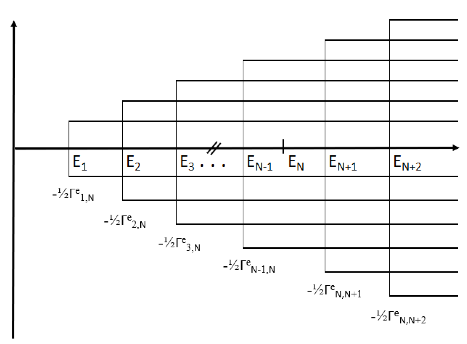
The partial shift $f_n(N;E_N)$ represents the contribution to the shift in level N from virtual transitions from level N to level n. We replace $E_N$ by the complex variable z and investigate the structure of the partial shift as a function of z:

$$f_n(N;z)=\frac{1}{\pi }{\int }_{E_n}^{E_n+{\omega }_c}d\omega \frac{-\frac{1}{2}{\Gamma }_{n,N}^e}{\omega -z-iϵ}.$$

(127)

We extend the lower limit of integration to $E_1$ and the upper limit to ∞ and multiply by the appropriate theta functions $\left(\theta \right(t)=0\mathrm{if}t<0,=1\mathrm{if}t>0)$ so that the value of the integral is unchanged. After summing over all states, we find that the complex radiative shift obeys the dispersion relation [28]

$$f(N;z)=\frac{1}{\pi }{\int }_{E_1}^{\infty }d\omega \frac{Imf(N;\omega )}{\omega -z-iϵ},$$

(128)

where

$$\mathrm{Im}f(N;z)=\sum _n^s-\frac{1}{2}{\Gamma }_{n,N}^e\theta (\omega -E_n)\theta ({\omega }_c+E_n-\omega ).$$

(129)

We can separate the integral into its real and imaginary parts

$$f(N;z)=\frac{1}{\pi }P{\int }_{E_1}^{\infty }d\omega \frac{\mathrm{Im}f(N;\omega )}{\omega -z}+iImf(N;z).$$

(130)

Figure 9 shows the cut structure for $f(N;\omega )$ in the complex $\omega$ plane.

5.2.2. Radiative Shift for Physical Energy Levels

The function ${f(N;z)|}_{z=E_N}$ gives the radiative shift for the energy level $E_N$. The imaginary part of the shift is

$$\begin{array}{cc}\hfill \mathrm{Im}\Delta E_N& =\mathrm{Im}f\left(N;E_N\right)\hfill \\ & =-\frac{1}{2}\sum _{n<N}{\Gamma }_{n,N}^e\equiv -\frac{1}{2}{\Gamma }_N,\hfill \end{array}$$

(131)

where ${\Gamma }_N$ is the total width for decay of state N by dipole radiation. The imaginary part of the shift equals the half-width in magnitude and is always negative as it must be to insure that the probability density decreases exponentially: $|e^{-it\left(E_N^0+\Delta E_N\right)}{|}^2=e^{-{\Gamma }_{N}t}$. Only states to which the state N can decay by the emission of real radiation contribute to the width of the level $E_N$.

The real part of the shift $\mathrm{Re}f(N;E_N)$ is given by the principal part of the integral. Since we integrate from $E_1$ to ∞, skipping the infinitesimal portion $|\omega -E_N|<ϵ$, all cuts (or equivalently all intermediate states) contribute to the real part of the radiative shift. Integrating over $\omega$ we obtain an expression for the real part of the partial shift $f_n(N;E_N)$:

$$\mathrm{Re}{f}_n(N;E_N)=\{\begin{array}{cc}-{\Gamma }_{n,N}^e\hfill & n<N\hfill \\ {\Gamma }_{N,n}^e\hfill & n>N\hfill \end{array}\times \frac{1}{2\pi }ln\frac{{\omega }_c-E_N+E_n}{\left|E_n-E_N\right|},$$

(132)

We can approximate Re$f_n(N;E_N)$ by neglecting $E_n-E_N$ in the numerator of the log. With this approximation, and writing the log of the ratio as a difference in logs, we can sum Re$f_n(N;E_N)$ over all states using the dipole sum rule:

$$\frac{3m^2}{2\alpha }\sum _n^s{\Gamma }_{N,n}^e=2\sum _n^s\left(E_n-E_N\right)〈N\left|p_i|n\rangle 〈n\left|p_i\right|N〉\right.=-\langle N|{\nabla }^{2}V|N\rangle .$$

(133)

This gives the result

$$\begin{array}{cc}\hfill Re\Delta E_N& =\frac{2\alpha }{3\pi m^2}\left\{\frac{1}{2}\langle N|{\nabla }^{2}V|N\rangle ln\frac{{\omega }_c}{E_0}\right.\hfill \\ & \left.+\sum _n\left(E_n-E_N\right)〈N\left|p_i\right|n〉〈n\left|p_i\right|N〉\ln \frac{E_0}{\left|E_n-E_N\right|}\right\},\hfill \end{array}$$

(134)

where $E_0$ is an arbitrary energy parameter, which we shall take to be some characteristic energy of the bound system, for example, the ground state energy. The first term is the same expression for the shift that we obtained by considering the motion of the particle in the zero-point field (Equation (29)). Note that we only assume the spinless electron is in a central force potential $V\left(r\right)$.

5.2.3. A Model to Interpret the Results

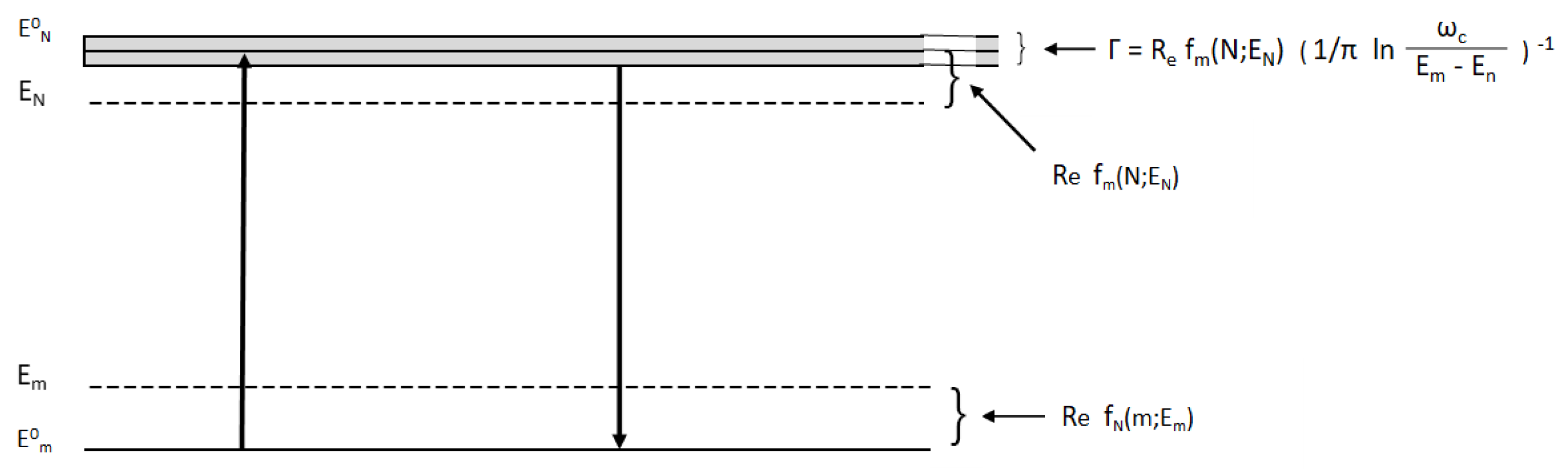
We can construct a simple model (Figure 10) to interpret the salient features of the partial radiative shifts $f_m(N;E_N)$, which give the shift in the energy $E_N$ due to virtual transitions to level m. The features are expressed in the following relations, which hold for any positive integer $m<N$:

(1)

Re$f_m(N;E_N)+\mathrm{Re}{f}_N(m;E_m)=0$.

(2)

Re $f_m(N;E_N)<0$.

(3)

Im $f_m(N;E_N)=\mathrm{Re}{f}_m(N;E_N){[\frac{1}{\pi }ln\frac{{\omega }_c}{E_N-E_m}]}^{-1}$.

The first relation shows that the average energy of two levels that shift each other is unchanged. Together, the first two relations show that virtual transitions to lower states cause downward shifts and transitions to upper states cause upward shifts. The third statement shows that a lower level’s contribution to the width is less than its contribution to the shift by the factor $\frac{1}{\pi }ln(\frac{{\omega }_c}{E_N-E_m})$. We can deduce relations (1) and (2) for the level shifts exactly and relation (3) for the level width in an approximation by assuming that the observed energy corresponds to a time-weighted average of the original energy and the energy of the state to which the system made a virtual transition. To make this interpretation quantitative, we consider a state N with a partial width $\Gamma ={\Gamma }_{N,m}^e={\Gamma }_{m,N}^a$ for $m<N$. The system makes $\Gamma$ transitions from N to m in one second and remains in the state m for a time allowed by the time-energy uncertainty principle [115]

$$\delta t\approx \frac{1}{E_N-E_m}.$$

(135)

Therefore, for a system in which $\Gamma <<E_N-E_m$ (e.g., atomic systems), the average energy $E_{N\mathrm{ave}}$ of level N is shifted and is approximately

$$E_{N\mathrm{ave}}=\frac{\Gamma }{E_N-E_m}{E}_m+\left(1-\frac{\Gamma }{E_N-E_m}\right)E_N=E_N-\Gamma .$$

(136)

The level shift for state N due to a transition from a state N to a lower state m is $E_{N\mathrm{ave}}-E_N$ or Re$f_m(N;E_N)=-{\Gamma }_{m,N}^e$. Similarly we find that for a transition from a state m to a higher state N the level shift is Re$f_N(m,E_N)={\Gamma }_{N,m}^a$ which is positive. From these two expressions, relations (1) and (2) follow. Corresponding to the third relation we find using Equation (129) and the results directly above that the model predicts a level width

$$\mathrm{Im}{f}_m(N;E_N)=-\frac{1}{2}\Gamma =\frac{1}{2}\mathrm{Re}{f}_m(N;E_N),$$

(137)

This result agrees with relation (3) only if we replace $\frac{1}{\pi }ln\frac{{\omega }_c}{E_N-E_m}$ by unity [116]. If we use the dipole sum rule, then in our model we find that the total level shift is $4/3$ of the result obtained in the discussion after Equation (37) where we obtained the shift by applying the uncertainty principle to determine the effects of the zero point field on a bound particle.

5.2.4. Two Examples: The Harmonic Oscillator and the Coulomb Potential

In our discussion thus far we only assume we have a spinless particle of mass m and charge e in a central force potential $V\left(r\right)$ interacting with its own radiation field. Now, we can apply the results to these two specific potentials.

(1) The Isotropic 3-D Harmonic Oscillator

Consider a simple isotropic harmonic oscillator in three dimensions for which

$$V\left(r\right)=\frac{1}{2}m{\omega }_0^2{r}^2,$$

(138)

with energy levels

$$E_N=(N+\frac{3}{2}){\omega }_0,N=n_1+n_2+n_3.$$

(139)

The fact that $V\left(r\right)$ increases formally with r without bound does not introduce difficulties since transitions are possible only between adjacent energy levels. Employing the matrix elements of the momentum operator

$$〈{n_i}^{\prime }\left|p_j\right|n_i〉=\sqrt{\frac{m{\omega }_0}{2}}\left(\sqrt{n_i+1}{\delta }_{n_i^{\prime }{n}_i+1}-\sqrt{n_i}{\delta }_{n_i^{\prime }{n}_i-1}\right),$$

(140)

we can easily compute the real and imaginary parts of the radiative shift using Equations (122), (123), (131) and (132). For the complex radiative shift of level $E_N$, we find

$$\Delta E_N=\frac{\alpha }{3\pi m}{\omega }_0^2\left(3ln\frac{{\omega }_C}{{\omega }_0}-i2\pi N\right),$$

(141)

giving a corresponding width

$${\Gamma }_N=\frac{2}{3}\frac{\alpha }{m}{\omega }_0^{2}N.$$

(142)

In the dipole approximation, the shift is the same for all levels: no degeneracy is split. On the other hand, the radiative width ${\Gamma }_N$ increases with N and agrees with the width Equation (12) obtained by applying the Bohr Correspondence Principle to the classical expression for the radiated power. The ratio of ${\Gamma }_N/E_N$ is constant and equals $(2/3)\alpha \hslash {\omega }_0/m{c}^2,$ In Section 6, we compute the radiative shift for a relativistic spinless electron and show that for some levels the degeneracy is lifted.

(2) The Coulomb Potential

We have

$$V\left(r\right)=-\frac{Z\alpha }{r},$$

(143)

and therefore

$${\nabla }^{2}V\left(r\right)=4\pi Z\alpha \delta \left(r\right).$$

(144)

Since the matrix elements vanish except for S states, we may isolate the L dependence of the shift by defining the Bethe log $\gamma (N,L)$ for a state characterized by principal quantum number N and angular momentum L [13]:

$$\begin{array}{c}\gamma (N,L)\sum _n^s\left(E_n-E_N\right)〈N0\left|p_i\right|n〉〈n\left|p_i\right|N0〉\hfill \\ =\sum _n^s\left(E_n-E_N\right)〈NL\left|p_i\right|n〉〈n\left|p_i\right|NL〉ln\frac{\left|E_n-E_N\right|}{\frac{1}{2}m{\left(Z\alpha \right)}^2}\hfill \end{array}.$$

(145)

Using Equation (134), setting the frequency cutoff to ${\omega }_c=m$, and substituting the Schrodinger wave function

$${\left|{\psi }_N\left(0\right)\right|}^2=\frac{1}{\pi }{\left(\frac{Z\alpha m}{N}\right)}^3{\delta }_{L0},$$

(146)

where the Kronecker delta function ${\delta }_{L0}$ vanishes if $L\ne 0$. We find for the shift for level $NL$

$$Re\Delta E_{NL}=\left[\frac{4m}{3\pi }\alpha {\left(Z\alpha \right)}^4\right]\frac{1}{N^3}\left\{{\delta }_{L0}ln\frac{2}{{\left(Z\alpha \right)}^2}-\gamma (N,L)\right\}.$$

(147)

where $\gamma (N,L)$ must still be numerically evaluated [117]. The result is the same result Bethe obtained in his original calculation. The Bethe log is tabulated for a few energy levels in the original work in which it is was introduced [13] and in various articles for additional levels and at a higher precision, for example [7,83].

To provide a scale of magnitude for the shift, we note that the term in square brackets is the energy radiated in one revolution of the electron in the ground state according to the laws of classical physics and equals Planck’s constant times 1090 MHz. For $N=2$, the 2s shift is 1051.84 MHz. The currently accepted value for the Lamb shift is about 1057.87 MHz. We can estimate

$$\Delta E_N/E_N\approx \alpha \frac{{\left(Z\alpha \right)}^2}{N},$$

(148)

which is about 1 part in 1.3 ×${10}^6$ for $N=2$. The width for low-lying states may be obtained by computing the sum in Equation (129) explicitly.

In the limit of very large quantum numbers for any central force field for circular orbits, we can simplify the expression for the width ${\Gamma }_N$ by assuming that the most important transitions are those for which $\Delta n<<N$. The strongest transitions in the classical limit are between wave packets corresponding to the circular orbits $n=N,l=N-1$ and $n=N-1,l=N-2$. This is equivalent to saying that the classical radiation is primarily in the fundamental band. Accordingly, our sum collapses to

$${\Gamma }_N={\omega }_{\mathrm{cl}}〈N\left|p_i\right|N-1〉〈N-1\left|p_i\right|N〉\frac{4\alpha }{3m^2},$$

(149)

where ${\omega }_{\mathrm{cl}}$ is the classical frequency of rotation. This matrix element can be obtained without direct computation by noting that

$$〈{N|p}^2|N〉\cong 〈N\left|p_i\right|N+1〉〈N+1\left|p_i\right|N〉+〈N\left|p_i\right|N-1〉〈N-1\left|p_i\right|N〉,$$

(150)

which follows from our assumption that the only significant transitions are those for which $\Delta N=\pm 1$ and from the fact that $\langle N\left|p_i\right|N\rangle =0$ for a bound state. We assume that the matrix elements do not change rapidly with N, thus

$$〈N\left|p_i\right|N-1〉〈N-1\left|p_i\right|N〉\cong 〈N\left|p_i\right|N+1〉〈N+1\left|p_i\right|N〉.$$

(151)

Therefore, our final expression for ${\Gamma }_N$ is

$${\Gamma }_N=\frac{2\alpha }{3m^2}{\omega }_{\mathrm{cl}}〈N\left|p^2\right|N〉.$$

(152)

For the Coulomb potential ${\omega }_{\mathrm{cl}}=m{\left(Z\alpha \right)}^2/N^3$ (see Equations (14) and (17)), we find

$${\Gamma }_N=\frac{2}{3}m\alpha \frac{{\left(Z\alpha \right)}^4}{N^5},$$

(153)

which is in accordance with the result obtained through the correspondence principle Equation (18).

Note that nowhere in our derivation of Equation (152) do we specify the detailed nature of the central force. We only assume that the radiation was in the fundamental band, which is always true for classical circular orbits. Indeed, this equation agrees with the expression for $\Gamma$ obtained by applying the correspondence principle to the classical expression for the radiated power $P_c$ for any circular orbit of a charged particle

$$P_c=\frac{2}{3}\frac{\alpha }{m^2}{p}^2{\omega }_{\mathrm{cl}}^2,$$

(154)

namely

$$\Gamma =\frac{2}{3}\frac{\alpha }{m^2}{p}^2{\omega }_{\mathrm{cl}}.$$

(155)

For both examples, the relative shifts go approximately as $\alpha$(Bound State Energy Level)/(Rest Mass Energy), reflecting the fundamental nature of radiative shifts (and that we are considering radiative shifts in lowest order).

For exact nonrelativistic calculations, the sum over states for the real part of the energy shift was trivial to compute for the oscillator since only two intermediate states contribute. Alternatively, if we compute the shift from Equation (107) without inserting intermediate states, then from the equations of motion we can easily compute the contraction over $p_i$. We will follow this procedure in our calculations of the level shift for the relativistic harmonic oscillator in Section 6. Unfortunately, to secure exact results for the Coulomb potential is more difficult. If we use Equation (112), we must include an infinite number of intermediate states in our sum. If we do not use intermediate states but use Equation (107) directly, then we find that the equations of motion are intractable unless we use group theoretical techniques, which we will publish elsewhere [118].

6. Radiative Shift of a Relativistic Meson (Spinless Electron) with a Harmonic Interaction Lagrangian

6.1. Introduction

We compute the radiative shift for a spinless, relativistic meson with a charge e with a harmonic interaction Lagrangian $L_{\mathrm{int}}=V{\psi }^2$ where $\psi$ is the meson field and $V=C^2{r}^2$, and C is a real constant. From consideration of the equations of motion, we compute the the radiative shift of the energy levels that corresponds to the difference of the contribution to the mass renormalization from a mass m bound by the harmonic interaction and a free meson [119,120]. We derive an integral expression for the complex radiative shift to order $\alpha$ in the radiation field and to all orders in the binding field. In Section 6.2, we perform the computations after making the simplifying assumption that the virtual photon is spinless. In Section 6.3 we include the effects of spin.

We assume the unperturbed meson state $|N\rangle$ obeys the Klein–Gordon equation with the interaction term

$$(p^2-p_0^2+C^2{r}^2+m^2)|N\rangle =0.$$

(156)

The equations of motion can be written in the form

$$(H-E_N^0)|N\rangle =0,$$

(157)

where

$$H=\frac{p^2}{2m}+\frac{m}{2}{(\frac{C}{m})}^2{r}^2,$$

(158)

and

$$E_N^0=\frac{p_0^2-m^2}{2m}.$$

(159)

This form shows that the equations of motion are the same as those of a simple harmonic oscillator with frequency

$$\omega =C/m,$$

(160)

Accordingly, we know the unperturbed energy levels are

$$E_N^0=(N+\frac{3}{2})\omega ,$$

(161)

and

$$p_0^2=2(N+\frac{3}{2})C+m^2,$$

(162)

6.2. Relativistic Radiative Shift for a Scalar Photon Interaction

The shift is given by the equation

$$\Delta E_N=E_N-E_N^0=ig\int \frac{d^{4}k}{{\left(2\pi \right)}^4}\frac{1}{k^2}〈N\left|\frac{1}{D(\overrightarrow{k})-i{ϵ}^{\prime }}\right|N〉,$$

(163)

where $g=2m{e}^2$ and $D(\overrightarrow{k})$ is the inverse momentum space propagator for the bound meson:

$$D\left(\overrightarrow{k},k_0\right)=D\left(k\right)={(\overrightarrow{p}-\overrightarrow{k})}^2-{\left(p_0-k_0\right)}^2+C^2{r}^2+m^2.$$

(164)

We employ the integral representations

$$\frac{1}{k^2-iϵ}=i{\int }_0^{\infty }d\lambda e^{-i\lambda k^2-ϵ\lambda },\frac{1}{D\left(k\right)-i{ϵ}^{\prime }}=i{\int }_0^{\infty }dt{e}^{-itD\left(k\right)-{ϵ}^{\prime }t}.$$

(165)

By employing the translation operator in momentum space, we see that

$$e^{-itD\left(k\right)}=e^{i\overrightarrow{k}·\overrightarrow{r}}{e}^{-itD(\overrightarrow{0},k_0)}{e}^{-i\overrightarrow{k}·\overrightarrow{r}},$$

(166)

where

$$D\left(\overrightarrow{0},k_0\right)=2mH+m^2-{\left(p_0-k_0\right)}^2.$$

(167)

By applying the equations of motion for the canonical variables for an elapsed time equal to $mt$,

$$\begin{array}{c}{e}^{-itmH}{r}_i{e}^{itmH}=r_{i}cos\left(Ct\right)-p_{i}sin\left(Ct\right),\hfill \\ e^{-itmH}{p}_i{e}^{itmH}=p_{i}cos\left(Ct\right)+r_{i}sin\left(Ct\right).\hfill \end{array}$$

(168)

we can compute the translations in Equation (166) explicitly with the result

$$\begin{array}{c}\frac{1}{D\left(k\right)-i{ϵ}^{\prime }}=i{\int }_0^{\infty }dt{e}^{-itmH}{e}^{i2\overrightarrow{k}·\overrightarrow{p}\nu }{e}^{+itmH}\hfill \\ \times e^{-i\mu k^2}{e}^{-it\left(m^2-{\left(p_0-k_0\right)}^2\right)}{e}^{-{ϵ}^{\prime }t},\hfill \end{array}$$

(169)

where

$$\begin{array}{c}\mu =\frac{sin\left(Ct\right)cos\left(Ct\right)}{C},\hfill \\ \nu =\frac{sin\left(Ct\right)}{C}.\hfill \end{array}$$

(170)

The integration over the scalar photon momentum can be performed by completing the square, and employing the general formula

$${\int }_{-\infty }^{\infty }dx{e}^{\pm (ia{x}^2-2ibx)}=\frac{\pi }{a}{e}^{\mp \frac{b^2}{a}}{e}^{\pm i\frac{\pi }{4}}.$$

(171)

After taking matrix elements, we find that the shift is

$$\Delta E_{N_1{N}_2{N}_3}={\int }_0^{\infty }dt{\int }_0^{\infty }d\lambda {\sigma }_N{\mathsf{\Omega }}_{N_1{N}_2{N}_3},$$

(172)

where we have used the product representation for the three-dimensional harmonic oscillator states $|N_1{N}_2{N}_3\rangle =|N_1\rangle |N_2\rangle |N_3\rangle$ and $N=N_1+N_2+N_3$. The quantities ${\sigma }_N$ and $\mathsf{\Omega }$ are

$${\sigma }_N=-\frac{g}{16{\pi }^2}{(\lambda +t)}^{-\frac{1}{2}}{e}^{-i{p}_0^2\left(\frac{t^2}{t+\lambda }\right)},$$

(173)

$${\mathsf{\Omega }}_{N_1{N}_2{N}_3}={(\lambda +\mu )}^{-\frac{3}{2}}〈N_1{N}_2{N}_3\left|e^{i{\overrightarrow{p}}^2\left(\frac{{\nu }^2}{\lambda +\mu }\right)}\right|N_1{N}_2{N}_3〉.$$

(174)

We can calculate the matrix elements directly and express the results in terms of the quantity

$$\mathsf{\Omega }\left(j\right)=\frac{{\left(i{\nu }^{2}C\right)}^j}{{\left(\lambda +\mu -i{\nu }^{2}C\right)}^{j+\frac{3}{2}}}.$$

(175)

We find

$$\begin{array}{c}{\mathsf{\Omega }}_{000}=\mathsf{\Omega }\left(0\right),\hfill \\ {\mathsf{\Omega }}_{100}=\mathsf{\Omega }\left(0\right)+\mathsf{\Omega }\left(1\right),\hfill \\ {\mathsf{\Omega }}_{200}=\mathsf{\Omega }\left(0\right)+2\mathsf{\Omega }\left(1\right)+\frac{3}{2}\mathsf{\Omega }\left(2\right),\hfill \\ {\mathsf{\Omega }}_{110}=\mathsf{\Omega }\left(0\right)+2\mathsf{\Omega }\left(1\right)+\mathsf{\Omega }\left(2\right).\hfill \end{array}$$

(176)

The radiative shifts lift the degeneracy for some levels and this parameterization simplifies the calculation of shifts between degenerate levels. The free particle mass shift is contained in $\mathsf{\Omega }\left(0\right)$ to all orders. This follows by noting that, for $j>0$, as $C\to 0$

$$\underset{C\to 0}{lim}\mathsf{\Omega }\left(j\right)\to 0.$$

(177)

For calculations of the shift between the nondegenerate energy levels, we would use a different formulation, subtracting the free particle shift in the beginning. To check our equations, we consider the limit $C\to 0$, which should yield the free particle renormalization. In this limit we have $\mu \to t$ and $\nu \to t$ so the only nonvanishing $\mathsf{\Omega }$ is

$$\mathsf{\Omega }\left(0\right)\to {(\lambda +t)}^{-\frac{3}{2}}.$$

(178)

Substituting these quantities into the expression for the shift, we find

$$\Delta E_{\mathrm{free}}=-\frac{g}{16{\pi }^2}{\int }_0^{1}dy{\int }_0^{\infty }\frac{dt}{t}{e}^{-{im}^{2}yt},$$

(179)

where we have made the substitution

$$y=\frac{t}{t+\lambda }.$$

(180)

To avoid having a spurious imaginary term, we do not include the contribution from the pole at $t=0$, but start our integration at $t=ϵ$. Using the formula

$${\int }_{ϵ}^{\infty }dt\frac{e^{-iat}}{t}=-ln\left(ϵa\right)-\gamma ,$$

(181)

we find

$$\Delta E_{free}=\frac{g}{16{\pi }^2}ln\left(ϵm^2\right)+\gamma -1,$$

(182)

where $ϵ$ in the infinitesimal cutoff for the t integration and $\gamma$ is Euler’ constant. This result has the same structure as the conventional result with respect to the divergences. The finite parts depend on the values of the cutoffs and on the particular procedures used to evaluate the integrals. The infinite terms cancel in the calculation of measurable shifts and consequently have no direct physical significance.

The expression for the bound state shifts can be rewritten in terms of y and $\tau =2Ct$:

$$\begin{array}{c}\lambda +\mu -i{\nu }^{2}C=\frac{\tau }{2Cy}\left[1-\frac{y}{i\tau }\left(e^{-i\tau }+i\tau -1\right)\right],\\ i{\nu }^{2}C=\frac{1}{4iC}\left(e^{i\tau }+e^{-i\tau }-2\right),\\ \mu =\frac{1}{4iC}\left(e^{i\tau }-e^{-i\tau }\right).\end{array}$$

(183)

The integral used to calculate the shifts is

$$\Delta E_N\left(j\right)\equiv {\int }_0^{1}dy{\int }_0^{\infty }dt{\sigma }_N\mathsf{\Omega }\left(j\right),$$

(184)

which equals

$$\Delta E_N\left(j\right)=-\frac{g}{16{\pi }^2}\frac{1}{{\left(2i\right)}^j}{\int }_0^{1}dy{\int }_{2Cϵ}^{\infty }\frac{d\tau }{{\tau }^{j+1}}\frac{y^j{\left(e^{i\tau }+e^{-i\tau }-2\right)}^j{e}^{-iy\eta \tau }}{{\left[1-\frac{y}{i\tau }\left(e^{-i\tau }+i\tau -1\right)\right]}^{j+\frac{3}{2}}},$$

(185)

where the degree of coupling to the harmonic oscillator is given by the dimensionless parameter

$$\eta =\frac{p_0^2}{2C}.$$

(186)

The shift can be expressed as a single integral of a confluent hypergeometric function with two arguments. The structure is similar to that for H atom where the shift can also be expressed in terms of an integral over a confluent hypergeometric function [11].

6.3. Relativistic Radiative Shift for a Spin 1 Photon Interaction

The expression for the shift is

$$\Delta E_N=E_N-E_N^0=ig\int \frac{d^{4}k}{{\left(2\pi \right)}^4}\frac{1}{k^2-iϵ}〈N\left|T_{\mu }^{\mu }\right|N〉,$$

(187)

where

$$T_{\mu }^{\mu }={(2p-k)}_{\mu }\frac{1}{D\left(k\right)-iϵ}{(2p-k)}^{\mu }.$$

(188)

Executing the trace gives

$$\begin{array}{c}{T}_{\mu }^{\mu }=4\left[p_i\frac{1}{D\left(k\right)}{p}_i-p_0^2\frac{1}{D\left(k\right)}\right]-2\left\{\overrightarrow{p}·\overrightarrow{k},\frac{1}{D\left(k\right)}\right\}-4p_0{k}_0\frac{1}{D\left(k\right)}-\left({\overrightarrow{k}}^2-k_0^2\right)\frac{1}{D\left(k\right)}\hfill \end{array}.$$

(189)

We can derive expressions for each of these quantities in terms of our previous results by employing the Heisenberg equations of motion for $p_i$ and $q_i$ (Equation (168)) and also our form of the Klein–Gordon equation (Equation (156)). Our final result is

$$\begin{array}{cc}\hfill \Delta E_{N_1{N}_2{N}_3}& =4{\int }_0^{\infty }d\lambda {\int }_0^{\infty }dt\left[-p_0^2-C^2{\nu }^{2}2C\left(N+\frac{3}{2}\right)-3i\mu C^2\right.\hfill \\ & -p_0^2\frac{t}{t+\lambda }+\left(2\mu \nu C^2+\frac{\lambda }{\nu }\right)\frac{1}{2i}\frac{\partial }{\partial \nu }\hfill \\ & \left.+C^2{\nu }^2\left(2C^2{\nu }^2-1\right)\frac{1}{-i}\frac{\partial }{\partial (\lambda +\mu )}\right]{\sigma }_N{\mathsf{\Omega }}_{N_1{N}_2{N}_3}\hfill \\ & +\frac{1}{i}\int dt{\sigma }_N{\mathsf{\Omega }}_{N_1{N}_2{N}_3}{|}_{\lambda =0},\hfill \end{array}$$

(190)

where ${\sigma }_N$ and ${\mathsf{\Omega }}_{N_1{N}_2{N}_3}$ have the same meaning as before (Equations (173) and (174)).

7. Conclusions

We discuss the history of Lamb shift and Bethe’s pivotal calculation, and how it influenced the direction of theoretical physics for over half a century.

We discuss the general nature of radiative shifts of bound state energy levels, from the classical and the quantum perspectives, examining in some detail results for the harmonic oscillator and the hydrogen atom. The radiative shifts are complex, the real part being the level shift and the imaginary part being the level width. The shifts arise because of the emission and absorption of virtual photons which occurs due to interaction of the charged particle with its own radiation field, or, equivalently, with the vacuum zero-point fluctuations. We know vacuum fluctuations are affected by geometry and therefore radiative shifts differ from free space values for atoms in a cavity, for example, or near a surface [105,106,107,108,110,121]. Lamb shifts have even been used to model gravitational energy in black holes [122].

Today, the computation of radiative shifts and atomic energy levels can be done very precisely, from 1 part in ${10}^{12}$ to 1 part in ${10}^{15}$ for certain energy levels, the most precise computations for any physical system [20]. Today, the corresponding experiments demonstrate comparable precision. Some see the opportunity for developing metrology [123,124,125,126,127]. This favorable situation allows atomic systems to be a platform for the discovery of new physics beyond the standard model. Theoreticians are already calculating the effect on energy levels due to the quantization of space, the non-commutativity of space-time coordinates and space-time fluctuations for H atoms, muonic atoms and Rydberg states [128,129,130,131,132,133,134,135]. Measurements are being done on collaborative Lamb shifts for mesoscopic arrays [136,137].

Because of this high precision, measurements of radiative shifts and atomic energy levels reveal detailed information about phenomena causing shifts aside from radiative effects. This precision has led to a new understanding low Z two body systems, including muonium, positronium, and tritium, revealing nuclear structure effects and other higher order effects. We can expect that atomic energy level measurements and computations will continue to contribute significantly to the development of quantum physics in the future.

References and Notes

- Eides, M.I.; Grotch, H.; Shelyoto, V. Theory of Light Hydrogenic Bound States; Springer Tracts in Modern Physics; Springer: Berlin, Germany, 2007. [Google Scholar]
- Springer Handbook of Atomic, Molecular and Optical Physics; Drake, G.W.F. (Ed.) Springer: New York, NY, USA, 2006. [Google Scholar]
- Karshenboim, S.G. Precision physics of simple atoms: QED tests, nuclear structure and fundamental constants. Phys. Rep. 2005, 422, 1–63. [Google Scholar] [CrossRef] [Green Version]
- Karshenboim, S.G. Simple Atoms, Quantum Electrodynamics, and Fundamental Constants. In Precision Physics of Simple Atomic Systems; Karshenboim, S.G., Smirnov, V.B., Eds.; Springer: Berlin/Heidelberg, Germany, 2003; pp. 141–162. [Google Scholar]
- Grotch, H.; Owen, D.A. Bound States in Quantum Electrodynamics: Theory and Application. Found. Phys. 2002, 32, 1419–1457. [Google Scholar] [CrossRef]
- Karshenboim, S.; Pavone, F.; Bassani, F.; Inguscio, M.; Hänsch, T.; Smirnov, V. (Eds.) The Hydrogen Atom: Precision Physics of Simple Atomic Systems; Springer: Berlin/Heidelberg, Germany, 2001. [Google Scholar]
- Eides, M.I.; Grotch, H.; Shelyoto, V. Theory of light hydrogenic atoms. Phys. Rep. 2001, 342, 63–261. [Google Scholar] [CrossRef] [Green Version]
- Grotch, H. Status of the Theory of the Hydrogen Lamb Shift. Found. Phys. 1994, 24, 249–272. [Google Scholar] [CrossRef]
- Sapirstein, J.; Yennie, D. Theory of Hydrogenic Bound States. Quantum Electrodynamics; Kinoshita, T., Ed.; World Scientific: Singapore, 1990; Both perturbative and nonperturbative approaches to the self-energy calculations as well as recoil corrections are summarized in the article by J. Sapirstein and D. Yennie. [Google Scholar]
- Szafron, R. Radiative Corrections in Bound States. Acta Phys. Pol. B 2017, 48, 2183. [Google Scholar] [CrossRef]
- Labzowsky, L.; Solovyev, D. Coulomb Green function and Its Application in Atomic Theory. Precision Physics of Simple Atomic Systems; Karshenboim, S.G., Smirnov, V.B., Eds.; Springer: Berlin/Heidelberg, Germany, 2003; pp. 141–162. [Google Scholar]
- Erickson, G.; Yennie, D. Radiative Level Shifts, I. Formulation and Lowest Order Lamb Shift. Ann. Phys. 1965, 36, 271–313. [Google Scholar] [CrossRef]
- Bethe, H.; Salpeter, E. The Quantum Mechanics of One and Two Electron Atoms; Springer: Berlin, Germany, 1957. [Google Scholar]
- Lamb, W.; Retherford, R. Fine Structure of the Hydrogen Atom by a Microwave Method. Phys. Rev. 1947, 72, 241. [Google Scholar] [CrossRef]
- Lamb, W.; Retherford, R. Fine Structure of the H Atom, Part I. Phys. Rev. 1950, 79, 549. [Google Scholar] [CrossRef]
- Lamb, W.; Retherford, R. Fine Structure of the H Atom, Part II. Phys. Rev. 1951, 81, 222. [Google Scholar] [CrossRef]
- Lamb, W.; Retherford, R. Fine Structure of the H Atom, Part III. Phys. Rev. 1952, 85, 259. [Google Scholar] [CrossRef]
- Lamb, W.; Retherford, R. Fine Structure of the H Atom, Part IV. Phys. Rev. 1952, 86, 1014. [Google Scholar] [CrossRef]
- Bethe, H. The Electromagnetic Shift of Energy Levels. Phys. Rev. 1947, 72, 339. [Google Scholar] [CrossRef]
- Beyer, A.; Maisenbacher, L.; Matveev, A.; Pohl, R.; Khabarova, K.; Grinin, A.; Lamour, T.; Yost, D.C.; Hänsch, T.W.; Kolachevsky, N.; et al. The Rydberg constant and proton size from atomic hydrogen. Science 2017, 358, 79–85. [Google Scholar] [CrossRef] [PubMed] [Green Version]
- Mohr, P.J.; Newell, D.B.; Taylor, B.N. CODATA recommended values of the fundamental physical constants: 2014. Rev. Mod. Phys. 2016, 88, 035009. [Google Scholar] [CrossRef] [Green Version]
- Babb, J.F.; Brickhouse, N. (Eds.) Eleventh International Conference on Atomic and Molecular Data and Their Applications; MDPI: Basel, Switzerland, 2020. [Google Scholar] [CrossRef]
- Milonni, P. The Quantum Vacuum; Academic Press: San Diego, CA, USA, 1994; Chapters 3,4 and 11 provide an excellent derivation and discussion of renormalization, radiative reaction, and the Lamb shift. [Google Scholar]
- Milonni, P. An Introduction to Quantum Optics and Quantum Fluctuations; Oxford Univ. Press: Oxford, UK, 2019; Chapter 4 of the excellent new book gives a careful and complete discussion of radiative shifts. [Google Scholar]
- Weinberg, S. The Quantum Theory of Fields; Cambridge Univesity Press: Cambridge, UK, 1995; Volume 1. [Google Scholar]
- Brown, L. Quantum Field Theory; Cambridge Univ. Press: Cambridge, UK, 1992. [Google Scholar]
- Bjorken, J.; Drell, S. Relativistic Quantum Mechanics; McGraw Hill: Neywork, NY, USA, 1964; Classic discussion of remormalization in terms of Feynman diagrams. [Google Scholar]
- Low, F. Natural Line Shape. Phys. Rev. 1952, 88, 53. [Google Scholar] [CrossRef]
- Oppenheimer, J.R. Note on the Theory of the Interaction of Field and Matter. Phys. Rev. 1930, 35, 461. [Google Scholar] [CrossRef]
- Kramers, H.A. Subtraction of infinities. Nuovo Cim. 1938, 15, 108. [Google Scholar] [CrossRef]
- Calculating the Lamb Shift, Videos 104-107 of Hans Bethe Scientist. Recorded by Sam Schweber. December 1996. Available online: webofstories.com (accessed on 15 March 2020).
- Salam, A.; Bethe, H.; Dirac, P.; Heisenberg, W.; Wigner, E.; Klein, O.; Lifshitz, E. Energy on Earth and in the Stars. In From a Life in Physics; World Scientific: Singapore, 1989. [Google Scholar]
- Weisskopf, V. The Development of Field Theory in the Last 50 Years. Phys. Today 1981, 34, 69–85. [Google Scholar] [CrossRef]
- Weisskopf, V. On the Self-Energy and the Electromagnetic Field of the Electron. Phys. Rev. 1939, 56, 72. [Google Scholar] [CrossRef]
- Isidor Isaac Rabi was awarded the 1944 Nobel Prize in physics for his development of the atomic and molecular beam magnetic resonance method of observing atomic spectra.
- Videos of Freeman Dyson 64-65 discussing Hans Bethe. Recorded by Sam Schweber. June 1998. Available online: webofstories.com (accessed on 15 March 2020).
- Dyson, F. Hans Bethe and Quantum Electrodynamics. Phys. Today 2005, 58, 48–51. [Google Scholar] [CrossRef] [Green Version]
- Feynman, R. The Development of the Space-Time View of Quantum Electrodynamics. Phys. Today 1966, 19, 31. [Google Scholar] [CrossRef] [Green Version]
- Schweber, S. QED and the Men Who Made It: Dyson, Feynman, Schwinger, and Tomonaga; Princeton Univ. Press: Princeton, NJ, USA, 1994. [Google Scholar]
- We generally employ natural Gaussian units so ℏ = 1, c = 1, and α = (e2/ℏc) ≈ 1/137. The notation for indices is μ,ν,…=0, 1, 2, 3; i, j,. = 1,2,3; pμpμ = − + . Occasionally we will show factors of ℏ and c for clarity.
- Serber, R. Linear Modifications in the Maxwell Field Equations. Phys. Rev. 1935, 48, 49. [Google Scholar] [CrossRef]
- Uehling, E. Polarization Effects in the Positron Theory. Phys. Rev. 1935, 48, 55. [Google Scholar] [CrossRef]
- Dyson, F. The Electromagnetic Shift of Energy Levels. Phy. Rev. 1948, 73, 617. [Google Scholar] [CrossRef]
- French, J.; Weisskopf, V. The Electromagnetic Shift of Energy Levels. Phys.Rev. 1949, 75, 1240. [Google Scholar] [CrossRef]
- Kroll, N.; Lamb, W.E., Jr. On the Self-Energy of a Bound Electron. Phys. Rev. 1949, 75, 388. [Google Scholar] [CrossRef]
- Schwinger, J. Quantum electrodynamics. I. A covariant formulation. Phy. Rev. 1948, 74, 1439. [Google Scholar] [CrossRef]
- Dyson, F. The Radiation Theories of Tomonaga, Schwinger, and Feynman. Phys. Rev. 1949, 75, 486. [Google Scholar] [CrossRef]
- Dyson, F. The S-Matrix in Quantum Mechanics. Phy. Rev. 1949, 75, 1736. [Google Scholar] [CrossRef]
- Dyson, F. Makers of Patterns, An Autobiography through Letters; Liveright Publishing: New York, NY, USA, 2018. [Google Scholar]
- Welton, T. Some observable effects of the quantum-mechanical fluctuations of the electromagnetic field. Phys. Rev. 1948, 74, 1157. [Google Scholar] [CrossRef]
- Baranger, M.; Bethe, H.A.; Feynman, R.P. Relativistic Correction to the Lamb Shift. Phys. Rev. 1953, 92, 482. [Google Scholar] [CrossRef] [Green Version]
- Karplus, R.; Klein, A.; Schwinger, J. Electrodynamic Displacement of Atomic Energy Levels. II. Lamb Shift. Phys. Rev. 1952, 86, 288. [Google Scholar] [CrossRef]
- Wichmann, E.H.; Kroll, N.M. Vacuum Polarization in a Strong Coulomb Field. Phys. Rev. 1956, 101, 843. [Google Scholar] [CrossRef]
- Erickson, W. Improved Lamb-Shift Calculation for All Values of Zα. Phys. Rev. Lett. 1971, 27, 780. [Google Scholar] [CrossRef]
- Power, E.A. Zero-Point Energy and the Lamb Shift. Am. J. Phys. 1966, 34, 516. [Google Scholar] [CrossRef]
- Weisskopf, V. The Privilege of Being a Physicist; W.H Freeman and Co.: New York, NY, USA, 1989. [Google Scholar]
- Mohr, P.J.; Plunien, G.; Soff, G. QED corrections in heavy atoms. Phys. Rep. 1998, 293, 227. [Google Scholar] [CrossRef]
- Mohr, P.H. Self-energy correction to one-electron energy levels in a strong Coulomb field. Phys. Rev. A 1992, 46, 4421. [Google Scholar] [CrossRef]
- Karshenboim, S.G. The Lamb shift of excited S-levels in hydrogen and deuterium atoms. Z. Phys. D 1997, 39, 109. [Google Scholar] [CrossRef] [Green Version]
- Karshenboim, S.G. Two-loop logarithmic corrections in the hydrogen Lamb shift. J. Phys. B At. Mol. Opt. Phys. 1996, 29, L29–L31. [Google Scholar] [CrossRef]
- Berkeland, D.; Hind, E.; Boshierm, M. Precision optical measurement of lamb shifts in atomic hydrogen. Phys. Rev. Lett. 1995, 75, 2470. [Google Scholar] [CrossRef]
- Karshenboim, S.G. Lamb Shift in the Hydrogen-Atom—Leading Logarithmic Corrections. Phys. At. Nucl. 1995, 58, 649–653. [Google Scholar]
- Karshenboim, S.G. Lamb Shift in the Hydrogen-Atom—Lifetime of the 2P(1/2) Level. Phys. At. Nucl. 1995, 58, 835–838. [Google Scholar]
- Karshenboim, S.G. The Lamb Shift in the Hydrogen-Atom—Shift. Phys. At. Nucl. 1995, 58, 262–266. [Google Scholar]
- Eides, M.I.; Grotch, H. Corrections of order α2(Zα)4 and α2(Zα)6 to the Lamb shift. Phys. Rev. A 1995, 52, 3360. [Google Scholar] [CrossRef] [PubMed] [Green Version]
- Karshenboim, S.G. Lamb Shift in Hydrogen-Atom. JETP 1994, 79, 230–236. Available online: http://www.jetp.ac.ru/cgi-bin/dn/e_079_02_0230.pdf (accessed on 15 March 2020).
- Pachucki, K. Higher-Order Binding Corrections to the Lamb Shift. Ann. Phys. (NY) 1993, 226, 1–87. [Google Scholar] [CrossRef]
- Palchikov, V.G.; Sokolov, Y.L.; Yakovlev, V.P. Lifetime of the 2P State and Lamb Shift in the Hydrogen-Atom. JETP Lett. 1983, 38, 418–420. Available online: http://www.jetpletters.ac.ru/ps/1483/article_22631.pdf (accessed on 15 March 2020).
- Lundeen, S.R.; Pipkin, F.M. Measurement of the Lamb Shift in Hydrogen, n=2. Phys. Rev. Lett. 1981, 46, 232. [Google Scholar] [CrossRef]
- Drake, G. Quantum electrodynamic Effects in Few-Electron Atomic Systems. Adv. At. Mol. Phys. 1982, 18, 399. [Google Scholar]
- Grotch, H. Lamb Shift in Nonrelativistic Quantum Electrodynamics. Am. J. Phys. 1981, 49, 48–51. [Google Scholar] [CrossRef]
- Sapirstein, J. Higher-Order Binding Corrections to the Lamb Shift. Phys. Rev. Lett. 1981, 47, 1723. [Google Scholar] [CrossRef]
- Schwebel, S. Interaction Theory-Relativistic Hydrogen-Atom and the Lamb Shift. Int. J. Theor. Phys. 1978, 17, 931–939. [Google Scholar] [CrossRef]
- Davies, B. Note on the Lamb shift. Am. J. Phys. 1982, 50, 331. [Google Scholar] [CrossRef]
- Karshenboim, S.G.; Ozawa, A.; Ivanov, V.G. Higher-order logarithmic corrections and the two-loop self-energy of a 1s electron in hydrogen. Phys. Rev. A 2019, 100, 032515. [Google Scholar] [CrossRef]
- Karshenboim, S.G.; Shelyuto, V.A. Three-loop radiative corrections to the 1s Lamb shift in hydrogen. Phys. Rev. A 2019, 100, 032513. [Google Scholar] [CrossRef]
- Eides, M.I.; Shelyuto, V.A. Hard three-loop corrections to hyperfine splitting in positronium and muonium. Phys. Rev. D 2015, 92, 013010. [Google Scholar] [CrossRef] [Green Version]
- Noble, J.H.; Jentschura, U.D. Dirac equations with confining potentials. Int. J. Mod. Phys. A 2015, 30, 1550002. [Google Scholar] [CrossRef]
- Eides, M.I.; Shelyuto, V.A. Polarization operator contributions to the Lamb shift and hyperfine splitting. Phys. Rev. A 2003, 68, 042106. [Google Scholar] [CrossRef] [Green Version]
- Szafron, R.; Korzinin, E.Y.; Shelyuto, V.A.; Ivanov, V.G.; Karshenboim, S.G. Virtual Delbruck scattering and the Lamb shift in light hydrogenlike atoms. Phys. Rev. A 2019, 100, 032507, Preprint in arxiv:1909.04116. Many papers of Prof. Karshenboim and collaborators are available on Arxiv. [Google Scholar] [CrossRef] [Green Version]
- Zamastil, J.; Patkos, V. Self-energy of an electron bound in a Coulomb field. Phys. Rev. A 2013, 88, 032501. [Google Scholar] [CrossRef]
- Zamastil, J. Approximate numerical calculation of the self-energy of a bound electron. Ann. Phys. 2012, 327, 297–328. [Google Scholar] [CrossRef]
- Jentschura, U.D.; Mohr, P.J. Calculation of hydrogenic Bethe logarithms for Rydberg states. Phys. Rev. A 2005, 72, 012110. [Google Scholar] [CrossRef] [Green Version]
- Jentschura, U.D. Techniques in analytic Lamb shift calculations. Mod. Phys. Lett. A 2005, 20, 2261–2276. [Google Scholar] [CrossRef] [Green Version]
- Jentschura, U.D.; Mohr, P.J.; Soff, G. Electron self-energy for the K and L shells at low nuclear charge. Phys. Rev. A 2001, 63, 042512. [Google Scholar] [CrossRef] [Green Version]
- Jentschura, U.D.; Mohr, P.J. Electron self-energy for higher excited S levels. Phys. Rev. A 2004, 69, 064103. [Google Scholar] [CrossRef] [Green Version]
- Eides, M.I.; Grotch, H.; Shelyuto, V.A. Radiative-recoil corrections of order α(Zα)5(m/M)m to the Lamb shift revisited. Phys. Rev. A 2002, 63, 052509. [Google Scholar] [CrossRef] [Green Version]
- Holstein, B.R. Effective interactions and the hydrogen atom. Am. J. Phys. 2004, 72, 333–344. [Google Scholar] [CrossRef]
- Jentschura, U.D.; Bigot, E.O.L.; Evers, J.; Mohr, P.J.; Keitel, C.H. Relativistic and radiative energy shifts for Rydberg states. J. Phys. B At. Mol. Opt. Phys. 2005, 38, S97–S105. [Google Scholar] [CrossRef] [Green Version]
- Agafonov, A.I. Hydrogen energy-level shifts induced by the atom motion: Crossover from the Lamb shifts to the motion-induced shifts. Mod. Phys. Lett. B 2018, 32, 1850273. [Google Scholar] [CrossRef] [Green Version]
- Kelkar, G.; Mart, T.; Nowakowski, M. Extraction of the Proton Charge Radius from Experiments. Makara J. Sci. 2016, 20, 119–126. [Google Scholar] [CrossRef]
- Martynenko, A.P. Proton-polarizability effect in the lamb shift for the hydrogen atom. Phys. At. Nucl. 2006, 69, 1309–1316. [Google Scholar] [CrossRef] [Green Version]
- The Alpha Collaboration. Investigation of the fine structure of antihydrogen, Nature 2020, 578, 375–380. [CrossRef] [Green Version]
- Feynman, R. QED The strange theory of light and matter; Princeton University Press: Princeton, NJ, USA, 1988; p. 128. [Google Scholar]
- The quantization volume V is an artifice to avoid infinite volumes. In this box normalization kx = 2πnx/Lx, ky = 2πny/Ly, and kz = 2πnz/Lz, with V = LxLyLz, and the integers nx, ny, and nz go from −∞ to +∞.
- Jackson, J. Classical Electrodynamics; Wiley and Sons: New York, NY, USA, 1962; Chapter 17. [Google Scholar]
- The classical radius of the electron is rcl = e2/(mc2) = 2.8 × 10⁻¹³ cm, which can be written at αℏ/mc = αƛ where ƛ is the reduced Compton wavelength of the electron 3.8 × 10⁻¹¹ cm (Compton wavelength divided by 2π).
- Cole, D.; Zou, Y. Quantum mechanical ground state of hydrogen obtained from classical electrodynamics. Phys. Lett. A 2003, 317, 14–20. [Google Scholar] [CrossRef] [Green Version]
- Boyer, T. Classical Zero-Point Radiation and Relativity:The Problem of Atomic Collapse Revisited. Found. Phys. 2016, 46, 880–890. [Google Scholar] [CrossRef] [Green Version]
- An alternative theory to quantum mechanics, Stochastic Electrodynamics (SED) posits that the vacuum fluctuations are a real, not a virtual, electromagnetic field, and that this field provides the energy lost by radiation and is responsible for the stability of atoms. See [98,99] for information on SED and atomic stability. For a critical evaluation for the H atom see Maclay, J. The Role of Vacuum Fluctuations and Symmetry in the Hydrogen Atom in Quantum Mechanics and Stochastic Electrodynamics. Atoms 2019, 7, 39. [Google Scholar] [CrossRef] [Green Version]
- We also mention the vacuum fluctuations of the charge density, characterized by virtual electron-positron pairs, which leads to the renormalization of the electron charge. Since this charge renormalization contributes much less to the shift between states than the mass renormalization from the zero point vibrations of the EM field, we shall not consider it here. In mesic atoms, in which the meson orbit is largely within the nucleus, the conversé situation obtains.
- Weisskopf, V. Recent Developments in the Theory of the Electron. Rev. Mod. Phys. 1949, 21, 305. [Google Scholar] [CrossRef]
- This expansion is essentially the dipole approximation.
- The metric is (−1, 1, 1, 1) for μ = 0, 1, 2, 3.
- Barton, G. New Aspects of the Casimir Effect: Fluctuations and Radiative Reaction. In Cavity Quantum Electrodynamics; Berman, P., Ed.; Academic Press: San Diego, CA, USA, 1994; pp. 425–455, This gives a clear discussion of how changes in the vacuum field due to surfaces affect charge, magnetic moment, mass and energy levels. [Google Scholar]
- Bordag, M.; Klimchitskaya, G.; Mohideen, U.; Mostepanenko, V. Advances in the Casimir Effect; Oxford Univ. Press: New York, NY, USA, 2009; This book gives a very complete discussion of how surfaces affect vacuum energy and can lead to Casimir forces between surfaces. [Google Scholar]
- Milton, K. The Casimir Effect, Physical Manifestations of Zero-Point Energy; World Scientific: Singapore, 2001. [Google Scholar]
- Milton, K.; Bordag, M. (Eds.) Quantum Field Theory Under the Influence of External Conditions; World Scientific: Singapore, 2010; This book discusses a broad variety of systems, including gravitational and nuclear. [Google Scholar]
- The shift is also temperature dependent since the vacuum field has a temperature dependent component.
- Billaud, B.; Truong, T.-T. Lamb shift of non-degenerate energy level systems placed between two infinite parallel conducting plates. J. Phys. A Math. Theor. 2013, 46, 025306. [Google Scholar] [CrossRef] [Green Version]
- Maclay, J. The Symmetry of the Energy Levels of the Hydrogen Atom and the Application of the Symmetry to the Calculation of Radiative Level Shifts. Ph.D. Thesis, Yale University, New Haven, CN, USA, 1972. [Google Scholar]
- The primes indicate eigenvalues of operators, and unprimed quantities indicate abstract operators. The quantity x′ means the four-vector (t′, ) and the volume element is d4x′ = dt′dx′dy′dz′. The partial derivative is defined as ∂′ = ∂/∂x′, and ∂′2 = −∂2/∂2t′ + ∂2/∂2x′ + ∂2/∂2y′ + ∂2/∂2z′. We also may write this operator as = −∂2/∂2 + ∂2/∂2 + ∂2/∂2 + ∂2/∂2 for an arbitrary four-vector ξ.
- To validate this expression for Gc we operate on the integral with Π′2 + m2. We observe Π′k < r′| =< r′|Πk, Π′0 < r′| =< r′|Π0 so (Π′2 + m2) < r′| =< r′|(Π2 + m2). With the normalization < r′|r″ >= δ(r′−r″), it follows the integral obeys the defining equation for Gc.
- Note that the sign of the energy shift is positive. This seems to contradict the rule that a perturbation must lower the ground state energy. The rule holds, however, if we consider the total perturbation to be the unrenormalized (mass)2 operator not the renormalized operator.
- The time-energy relationship is not an uncertainly principle in the same sense as the position-momentum uncertainty principle, which follows because the corresponding operators do not commute. The time-energy relationship arises from the properties of Fourier transforms and is consistent with the position-momentum uncertainty principle.
- For the H atom, the value of (1/π) ln((En − Em)/ωc) is roughly −3 assuming the cutoff is at hωc = mc2 and n and m are adjacent bound state energy levels.
- The Bethe log is commonly written as ln (K0/Z2Ry) where K0 refers to the average excitation energy [EN − Em]ave, and Ry is the Rydberg constant.
- Maclay, J., Revisiting the Symmetry of the H Atom: SO(4) to SO(4,2), and Its Use to Calculate Radiative Shifts, to be submitted for publication in 2020 in the upcoming special issue on “Symmetries in Quantum Mechanics” of the open access journal Symmetry.
- Došlić, N.; Danko, S. Harmonic oscillator with the radiation reaction interaction. Phys. Rev. A 1995, 51, 3485. [Google Scholar]
- Daeimohamad, M.; Mohammadi, M. Quantum Dynamics of a Harmonic Oscillator in a Deformed Bath in the Presence of Lamb Shift. Int. J. Theor. Phys. 2012, 51, 3052–3061. [Google Scholar] [CrossRef]
- Koshino, K.; Nakamura, Y. Control of the radiative level shift and linewidth of a superconducting artificial atom through a variable boundary condition. New J. Phys. 2012, 14, 043005. [Google Scholar] [CrossRef]
- Porto, R.A. Lamb shift and the gravitational binding energy for binary black holes. Phys. Rev. D 2017, 96, 024063. [Google Scholar] [CrossRef] [Green Version]
- Cagnac, B. Hydrogen metrology: Up to what limit? Phys. Scr. 1997, T70, 24–33. [Google Scholar] [CrossRef]
- Cagnac, B. Progress on the Rydberg Constant—THE Hydeogen-Atom as a Freauency Standard. IEEE Trans. Instrum. Meas. 1993, 42, 206–213. [Google Scholar] [CrossRef]
- Cagnac, B.; Plimmer, M.D.; Julien, L.; Biraben, F. The Hydrogen-Atom, a Tool for Metrology. Rep. Prog. Phys. 1994, 57, 853–893. [Google Scholar] [CrossRef]
- Hagel, G.; Schwob, C.; Jozefowski, L.; de Beauvoir, B.; Hilico, L.; Nez, F.; Julien, L.; Biraben, F.; Acef, O.; Clairon, A. Metrology of hydrogen atom: Determination of the Rydberg constant and Lamb shifts. Laser Phys. 2001, 11, 1076–1082. [Google Scholar]
- Mohr, P.; Taylor, B. Quantum electrodynamics and the fundamental constants. Adv. Quantum Chem. 1998, 30, 77–97. [Google Scholar]
- Jones, M.; Potvliege, R.M.; Spannowsky, M. Probing new physics using Rydberg states of atomic hydrogen. Phys. Rev. Res. 2020, 2, 013244. [Google Scholar] [CrossRef] [Green Version]
- Alavi, A.; Rezaei, N. Dirac equation, hydrogen atom spectrum and the Lamb shift in dynamical non-commutative spaces. Pramana J. Phys. 2017, 88, 77. [Google Scholar] [CrossRef]
- Haghighat, M.; Khorsandi, M. Hydrogen and muonic hydrogen atomic spectra in non-commutative space-time. Eur. Phys. J. C 2015, 75, 4. [Google Scholar] [CrossRef] [Green Version]
- Gnatenko, K.P.; Krynytskyi, Y.S.; Tkachuk, V.M. Perturbation of the ns levels of the hydrogen atom in rotationally invariant noncommutative space. Mod. Phys. Lett. A 2015, 30, 1550033. [Google Scholar] [CrossRef] [Green Version]
- Rivas, I.; Camacho, A.; Goklu, E. Quantum spacetime fluctuations: Lamb shift and hyperfine structure of the hydrogen atom. Phys. Rev. D 2011, 84, 055024. [Google Scholar] [CrossRef] [Green Version]
- Zaim, S.; Khodja, L.; Delenda, Y. Second-Order Corrections to the Noncommutative Klein-Gordon Equation with a Coulomb Potential. Int. J. Mod. Phys. A 2011, 26, 4133–4144. [Google Scholar] [CrossRef] [Green Version]
- Bouaziz, D.; Ferkous, N. Hydrogen atom in momentum space with a minimal length. Phys. Rev. A 2010, 82, 022105. [Google Scholar] [CrossRef] [Green Version]
- Chaichian, M.; Sheikh-Jabbari, M.M.; Tureanu, A. Hydrogen atom spectrum and the Lamb shift in noncommutative QED. Phys. Rev. Lett. 2001, 86, 2716–2719. [Google Scholar] [CrossRef] [PubMed] [Green Version]
- Scully, M.O. Collective Lamb shift in single photon Dicke superradiance. Phys. Rev. Lett. 2009, 102, 143601. [Google Scholar] [CrossRef]
- Meir, Z.; Schwartz, O.; Shahmoon, E.; Oron, D.; Ozeri, R. Cooperative Lamb Shift in a Mesocopic Atomic Array. Phy. Rev. Let. 2014, 113, 193002. [Google Scholar] [CrossRef] [Green Version]
- Milonni, P.; Theoretical Division, Los Alamos National Laboratory, Los Alamos, NM 87545, USA. Personal communication, 2020.
- Lamb, W. Super classical quantum mechanics: The best interpretation of nonrelativistic quantum mechanics. Am. J. Phys. 2001, 69, 413–422. [Google Scholar] [CrossRef]
- Schweber, S. The Happy Thirties. Phys. Today 2005, 58, 38. [Google Scholar] [CrossRef]
Figure 1.
Feynman diagrams for mass renormalization. Time axis is horizontal. The diagram on the left corresponds to the term and shows an electron emitting a virtual photon and then at a later time reabsorbing the photon. The diagram on the right corresponds to the term.
Figure 2.
Feynman diagrams for the bound state mass renormalization. The double line represents a meson bound in an external potential.
Figure 3.
Feynman diagrams showing the level shift is the difference between the bound state mass renormalization and the free particle mass renormalization. The double line represents a meson bound in an external potential.
Figure 4.
Feynman diagrams for the meson (top line) bound to the Coulomb field of a proton (bottom line). The dots indicate that all possible configurations of Coulomb photons, including crossed photon lines, are to be included.
Figure 5.
Feynman diagrams for the meson (top line) bound to the Coulomb field of a proton (bottom line), with the exchange of Coulomb photons and one radiative photon emitted and reabsorbed by the meson.
Figure 6.
Feynman diagram for lowest order radiative correction to the bound meson.
Figure 7.
Feynman diagrams for the Compton scattering amplitude of a photon by a bound meson (double line).
Figure 8.
Feynman diagrams for which give the radiative shift of a bound meson, which arise from the Compton scattering amplitude (Figure 7) of virtual radiation photons by a bound meson (double line).
Figure 9.
Cut Structure of in the complex plane. At each value of which is less than , there is a cut with a discontinuity of ; at , there is no cut. At each value of which is greater than , there is a cut with a discontinuity of .
Figure 10.
The energy level is shifted to by intermediate virtual transitions to , which also increases the width of the level to . The level is shifted to by virtual transitions to . The latter transition does not increase the width of the level for .
© 2020 by the author. Licensee MDPI, Basel, Switzerland. This article is an open access article distributed under the terms and conditions of the Creative Commons Attribution (CC BY) license (http://creativecommons.org/licenses/by/4.0/).
Share and Cite
MDPI and ACS Style
Maclay, G.J. History and Some Aspects of the Lamb Shift. Physics 2020, 2, 105-149. https://0-doi-org.brum.beds.ac.uk/10.3390/physics2020008
AMA Style
Maclay GJ. History and Some Aspects of the Lamb Shift. Physics. 2020; 2(2):105-149. https://0-doi-org.brum.beds.ac.uk/10.3390/physics2020008
Chicago/Turabian StyleMaclay, G. Jordan. 2020. "History and Some Aspects of the Lamb Shift" Physics 2, no. 2: 105-149. https://0-doi-org.brum.beds.ac.uk/10.3390/physics2020008