Warping Effects in Strongly Perturbed Metrics

Abstract

A technique devised some years ago permits us to develop a theory regarding a regime of strong perturbations. This translates into a gradient expansion that, at the leading order, can recover the Belinsky-Kalathnikov-Lifshitz solution for general relativity. We solve exactly the leading order Einstein equations in a spherical symmetric case, assuming a Schwarzschild metric under the effect of a time-dependent perturbation, and we show that the 4-velocity in such a case is multiplied by an exponential warp factor when the perturbation is properly applied. This factor is always greater than one. We will give a closed form solution of this factor for a simple case. Some numerical examples are also given.

1. Introduction

The study of Einstein equations in certain regimes is often restricted to solving them numerically [1]. The reason is that they form a set of nonlinear partial differential equations that are generally difficult to handle with analytical tools for most interesting situations. Often, the reason relies in the fact that no small parameter can be found to apply to standard perturbation techniques, while analytical solutions are very rare and difficult to find. Some years ago, a member of our group (Marco Frasca) proposed an approach based on earlier works on strongly perturbed systems [2]. It was shown that, under a strong perturbation in the formal limit running to infinity, the leading order is obtained by neglecting the gradient terms in the Einstein equations. The leading order of this perturbation series was firstly proposed by Belinsky, Kalathnikov, and Lifshitz for their famous BKL conjecture [3,4,5], as is known today.

Some decades ago, Alcubierre proposed a solution for the Einstein equations [6] that describes an observer moving with an unbounded velocity, provided that the condition of positivity of the energy is violated. A recent paper [7] (see also references therein) presents a short account of the Alcubierre metric and its interaction with dust. Indeed, many kinds of pathologies have emerged about it and the difficulties arise from the fact that this is an engineered metric that is imposed on the Einstein equations. It would be desirable to have a metric like this one emerging as a solution for the Einstein equations and conserving the positivity of the energy. A recent proposal works in such a direction [8]. This is possible by introducing a hyperbolic shift vector potential and the author shows how this can emerge from a plasma.

In this paper, we will show how a warp factor for the velocity can emerge when a strong perturbation is applied to a spherical symmetric metric. Thus, any Eulerian observer will have its velocity expanded when such perturbation acts. This extends and completes our preceding work [2]. We will obtain the exact solution for the leading perturbation equations and we will show how an exponential factor can emerge that is systematically greater than one. We emphasize that we are applying perturbation theory in a limit where the a perturbation applied to a given gravitational field is taken to be much greater than the unperturbed situation. This is the opposite limit to standard small perturbation theory and is based on the technique devised in [2].

The paper is so structured. In Section 2, we will introduce a technique to treat strongly perturbed systems. In Section 3, we apply this to the Einstein equations for a spherical symmetry metric with a time-dependent perturbation. In Section 4, we solve the leading order perturbation equations. In Section 5, we present the geodesic equations. In Section 6, we show how the expansion factor enters into the velocity, providing some examples and an analytic solution. In Section 7, conclusions are presented.

2. Strong Perturbations and Gradient Expansion

For our computations in general relativity, we need to study the case of a strong perturbation on a given metric: we select the Schwarzschild metric. In order to prove that a gradient expansion indeed represents a strong perturbation theory, we will study the following non-linear equation as a toy model for the Einstein equations that can represent Einstein equations in 1 + 1 dimensions [9,10,11]:

$$-\square \varphi +\lambda V^{\prime }\left(\varphi \right)=0,$$

(1)

where the prime means derivative with respect to $\varphi$, $\square ={\nabla }^2-{\partial }_t^2$ with ${\partial }_t$ being the time derivative, $\partial /\partial t$, is the wave operator, $\varphi$ is a scalar field and $V\left(\varphi \right)$ is its self-interaction with a coupling $\lambda$. Here and in what follows, the speed of light is set $c=1$. For 2-dimensional Einstein equations, this would be a Liouville equation [9,10,11]. We would like to apply perturbation theory in the formal limit of $\lambda \to \infty$. This results in a non-trivial series in $1/\lambda$. We can accomplish our aim by rescaling the time variable [12]. We take $t\to \sqrt{\lambda }t$ and the equation above becomes

$$-{\nabla }^2\varphi +\lambda {\partial }_t^2\varphi +\lambda V^{\prime }\left(\varphi \right)=0.$$

(2)

Then, we take

$$\varphi ={\varphi }_0+\frac{1}{\lambda }{\varphi }_1+\frac{1}{{\lambda }^2}{\varphi }_2+\dots$$

(3)

and substitute this into Equation (2). This gives the following set of perturbative equations:

$$\begin{array}{ccc}\hfill {\partial }_t^2{\varphi }_0& =& -V^{\prime }\left({\varphi }_0\right),\hfill \\ \hfill {\partial }_t^2{\varphi }_1& =& -V^{″}\left({\varphi }_0\right){\varphi }_1+{\nabla }^2{\varphi }_0,\hfill \\ \hfill {\partial }_t^2{\varphi }_2& =& -V^{″}\left({\varphi }_0\right){\varphi }_2-\frac{1}{2}{V}^{‴}\left({\varphi }_0\right){\varphi }_1^2+{\nabla }^2{\varphi }_1,\hfill \\ \hfill \mathrm{etc}.& & \end{array}$$

(4)

We see that we have obtained a set of non-trivial equations that define the perturbation series in the formal limit $\lambda \to \infty$. This approach can be applied, exactly in this way, to the Einstein equations. This also shows how consistent was the original BKL approach in [3,4,5]. Indeed, we have obtained a gradient expansion.

In order to see how this technique applies to Einstein equations, we express them in the Arnowitt–Deser–Misner (ADM) formalism as [1] (here and in the following Latin indexes $i,j,\dots$ run from 1 to 3, Greek indexes run from 0 to 3)

$$\begin{array}{ccc}\hfill {\partial }_t{\gamma }_{ij}-{\beta }^l{\partial }_l{\gamma }_{ij}& =& {\gamma }_{lj}{\partial }_i{\beta }^l+{\gamma }_{il}{\partial }_j{\beta }^l-2\alpha K_{ij},\hfill \end{array}$$

(5)

$$\begin{array}{ccc}\hfill {\partial }_t{K}_{ij}-{\beta }^l{\partial }_l{K}_{ij}& =& K_{il}{\partial }_j{\beta }^l+K_{jl}{\partial }_i{\beta }^l-2\alpha K_{il}{K}_j^l+\alpha K{K}_{ij}\hfill \\ \hfill & & -\frac{1}{2}\alpha {\gamma }^{lm}\left\{{\partial }_l{\partial }_m{\gamma }_{ij}+{\partial }_i{\partial }_j{\gamma }_{lm}-{\partial }_i{\partial }_l{\gamma }_{mj}-{\partial }_j{\partial }_l{\gamma }_{mi}\right.\hfill \\ \hfill & & +{\gamma }^{np}\left[({\partial }_i{\gamma }_{jn}+{\partial }_j{\gamma }_{in}-{\partial }_n{\gamma }_{ij}){\partial }_l{\gamma }_{mp}\right.\hfill \\ \hfill & & +{\partial }_l{\gamma }_{in}{\partial }_p{\gamma }_{jm}-{\partial }_l{\gamma }_{in}{\partial }_m{\gamma }_{jp}]\hfill \\ \hfill & & -\frac{1}{2}{\gamma }^{np}\left[({\partial }_i{\gamma }_{jn}+{\partial }_j{\gamma }_{in}-{\partial }_n{\gamma }_{ij}){\partial }_p{\gamma }_{lm}+{\partial }_i{\gamma }_{ln}{\partial }_j{\gamma }_{mp}]\right\}\hfill \\ \hfill & & -{\partial }_i{\partial }_j\alpha +\frac{1}{2}{\gamma }^{lm}({\partial }_i{\gamma }_{jm}+{\partial }_j{\gamma }_{im}-{\partial }_m{\gamma }_{ij}){\partial }_l\alpha \hfill \\ & & +\alpha \left[-8\pi G{T}_{ij}+4\pi G{\gamma }_{ij}(T-\rho )\right],\hfill \end{array}$$

(6)

where ${\partial }_i=\partial /\partial x^i$, G is the Newton constant and the energy–matter tensor $T_{ij}$ is given with the density $\rho$, for a metric

$$d{s}^2=(-{\alpha }^2+{\gamma }_{ij}{\beta }^i{\beta }^j)d{t}^2+2{\beta }^{i}d{x}_{i}dt+{\gamma }_{ij}d{x}^{i}d{x}^j$$

(7)

with $\alpha$ being the lapse function, ${\beta }^i$ the shift vector, ${\gamma }_{ij}$ the spatial part of the metric and $K_{ij}$ the extrinsic curvature. For our purposes, we are not interested in constraint equations that are essential only for numerical computations. This set is amenable to the same treatment we applied to the preceding example. The procedure is identical: we introduce an ordering parameter $\lambda$ that we will set to 1 to the end of computation. Then, we consider the perturbation series defined by

$$\begin{array}{ccc}\hfill \tau & =& \sqrt{\lambda }t,\hfill \\ \hfill K_{ij}& =& \sqrt{\lambda }\left(K_{ij}^{\left(0\right)}+\frac{1}{\lambda }{K}_{ij}^{\left(1\right)}+\frac{1}{{\lambda }^2}{K}_{ij}^{\left(2\right)}+\dots \right),\hfill \\ \hfill {\gamma }_{ij}& =& {\gamma }_{ij}^{\left(0\right)}+\frac{1}{\lambda }{\gamma }_{ij}^{\left(1\right)}+\frac{1}{{\lambda }^2}{\gamma }_{ij}^{\left(2\right)}+\dots ,\hfill \\ \hfill \alpha & =& {\alpha }_0+\frac{1}{\lambda }{\alpha }_1+\frac{1}{{\lambda }^2}{\alpha }_2+\dots .\hfill \end{array}$$

(8)

Our gauge choice is to set the shift vector ${\beta }_i=0$. This approach mirrors completely the standard computation for weak gravitational fields but implies that the perturbation is taken formally to reach infinity. This represents a situation where the perturbation overcomes the intensity of the gravitational field where it is applied. Typical situations where this technique could apply include black hole collisions, where, currently, only numerical computations or analytical techniques, working given certain approximations, are available [13]. Therefore, we obtain the following non-trivial set of equations (we have set $\lambda =1$):

$$\begin{array}{ccc}\hfill {\partial }_t{\gamma }_{ij}^{\left(0\right)}& =& -2{\alpha }_0{K}_{ij}^{\left(0\right)},\hfill \\ \hfill {\partial }_t{\gamma }_{ij}^{\left(1\right)}& =& -2{\alpha }_1{K}_{ij}^{\left(0\right)}-2{\alpha }_0{K}_{ij}^{\left(1\right)},\hfill \\ \hfill & ⋮& \end{array}$$

(9)

$$\begin{array}{ccc}\hfill {\partial }_t{K}_{ij}^{\left(0\right)}& =& -2{\alpha }_0{K}_{il}^{\left(0\right)}{K}_j^{l\left(0\right)}+{\alpha }_0{K}^{\left(0\right)}{K}_{ij}^{\left(0\right)}\hfill \\ \hfill {\partial }_t{K}_{ij}^{\left(1\right)}& =& -2{\alpha }_1{K}_{il}^{\left(0\right)}{K}_j^{l\left(0\right)}-2{\alpha }_0{K}_{il}^{\left(1\right)}{K}_j^{l\left(0\right)}-2{\alpha }_0{K}_{il}^{\left(0\right)}{K}_j^{l\left(1\right)}\hfill \\ \hfill & & +{\alpha }_1{K}^{\left(0\right)}{K}_{ij}^{\left(0\right)}+{\alpha }_0{K}^{\left(1\right)}{K}_{ij}^{\left(0\right)}+{\alpha }_0{K}^{\left(0\right)}{K}_{ij}^{\left(1\right)}\hfill \\ \hfill & & -\frac{1}{2}{\alpha }_0{\gamma }^{lm\left(0\right)}\left\{{\partial }_l{\partial }_m{\gamma }_{ij}^{\left(0\right)}+{\partial }_i{\partial }_j{\gamma }_{lm}^{\left(0\right)}-{\partial }_i{\partial }_l{\gamma }_{mj}^{\left(0\right)}-{\partial }_j{\partial }_l{\gamma }_{mi}^{\left(0\right)}\right.\hfill \\ \hfill & & +{\gamma }^{np\left(0\right)}\left[({\partial }_i{\gamma }_{jn}^{\left(0\right)}+{\partial }_j{\gamma }_{in}^{\left(0\right)}-{\partial }_n{\gamma }_{ij}^{\left(0\right)}){\partial }_l{\gamma }_{mp}^{\left(0\right)}\right.\hfill \\ \hfill & & +{\partial }_l{\gamma }_{in}^{\left(0\right)}{\partial }_p{\gamma }_{jm}^{\left(0\right)}-{\partial }_l{\gamma }_{in}^{\left(0\right)}{\partial }_m{\gamma }_{jp}^{\left(0\right)}]\hfill \\ \hfill & & -\frac{1}{2}{\gamma }^{np\left(0\right)}\left[({\partial }_i{\gamma }_{jn}^{\left(0\right)}+{\partial }_j{\gamma }_{in}^{\left(0\right)}-{\partial }_n{\gamma }_{ij}^{\left(0\right)}){\partial }_p{\gamma }_{lm}^{\left(0\right)}+{\partial }_i{\gamma }_{ln}^{\left(0\right)}{\partial }_j{\gamma }_{mp}^{\left(0\right)}]\right\}\hfill \\ \hfill & & -{\partial }_i{\partial }_j{\alpha }_0+\frac{1}{2}{\gamma }^{lm\left(0\right)}({\partial }_i{\gamma }_{jm}^{\left(0\right)}+{\partial }_j{\gamma }_{im}^{\left(0\right)}-{\partial }_m{\gamma }_{ij}^{\left(0\right)}){\partial }_l{\alpha }_0\hfill \\ \hfill & & +{\alpha }^{\left(0\right)}\left[-8\pi G{T}_{ij}+4\pi G{\gamma }_{ij}^{\left(0\right)}(T-\rho )\right],\hfill \\ \hfill \mathrm{etc}.\end{array}$$

(10)

where one sees that the energy–matter tensor contributes to the next-to-leading order. We realize from these equations that the gradient terms—that is, components of the metric that vary spatially—are moved to the next-to-leading order. We will apply them in the following in the spherical symmetric case, assuming the Schwarzschild metric as the unperturbed solution. Here, and in the following, we avoid showing explicitly the energy–matter tensor as our perturbation series moves its contribution to the next-to-leading order. This implies that, at the leading order, an approximation for the energy–matter configuration can be taken to be that in absence of the gravitational field. This is consistent with our approach for strongly perturbed metrics.

Nevertheless, in order to gain insight into the main concept underlying this approximation scheme, let us consider the Reissner–Nördstrom metric of a charged black hole. This will be given by

$$d{s}^2=-\left(1-\frac{r_g}{r}+\frac{r_Q^2}{r^2}\right)d{t}^2+{\left(1-\frac{r_g}{r}+\frac{r_Q^2}{r^2}\right)}^{-1}d{r}^2+r^{2}d{\theta }^2+r^2{sin}^2\theta d{\varphi }^2,$$

(11)

with $r_g=2GM$ being the Schwarzschild radius for a mass M and $r_q^2=G{Q}^2/4\pi {ϵ}_0$ the scale introduced by the black hole charge Q with $1/4\pi {ϵ}_0$ the Coulomb constant. This is an exact solution for the Einstein–Maxwell equations. In our case, we assume that the electric field overcomes largely the gravitational contribution—that is, $r_Q\gg r_g$. This appears formally as a large perturbation on a Schwarzschild black hole and the approximate metric will be

$$d{s}^2=-\left(1+\frac{r_Q^2}{r^2}\right)d{t}^2+{\left(1+\frac{r_Q^2}{r^2}\right)}^{-1}d{r}^2+r^{2}d{\theta }^2+r^2{sin}^2\theta d{\varphi }^2+\mathcal{O}(r_g/r).$$

(12)

This should be compared with the opposite dual limit $r_Q/r_g\ll 1$, which yields

$$d{s}^2=-\left(1-\frac{r_g}{r}\right)d{t}^2+{\left(1-\frac{r_g}{r}\right)}^{-1}d{r}^2+r^{2}d{\theta }^2+r^2{sin}^2\theta d{\varphi }^2+\mathcal{O}(r_Q^2/r^2).$$

(13)

3. Strongly Perturbed Spherical Symmetry Metric

We assume a spherical symmetry metric in ADM formalism given by

$$d{s}^2=-{\alpha }^{2}d{t}^2+{\gamma }_{rr}d{r}^2+{\gamma }_{\theta \theta }d{\theta }^2+{\gamma }_{\varphi \varphi }d{\varphi }^2.$$

(14)

This implies a specific choice of the gauge where all the components of the shift vector, normally named ${\beta }_i$, are taken to be zero. Then, the perturbation ${\alpha }_1$ is applied to the lapse function as follows [1]:

$${\alpha }^2={\alpha }_0^2+{\alpha }_1.$$

(15)

Then, we specialize the set of Equation (9) to this case. Assuming the Schwarzschild solution as the unperturbed solution, the exterior solution is given by (again, $r_g=2GM$ is the Schwarzschild radius)

$$\begin{array}{ccc}\hfill {\alpha }_0^2& =& \left(1-\frac{r_g}{r}\right),\hfill \\ \hfill {\gamma }_{11}^{\left(0\right)}& =& \frac{1}{1-\frac{r_g}{r}},\hfill \\ \hfill {\gamma }_{22}^{\left(0\right)}=r^2,& & {\gamma }_{33}^{\left(0\right)}=r^2{sin}^2\theta ,\hfill \end{array}$$

(16)

and the interior solution is

$$\begin{array}{ccc}\hfill {\alpha }_0^2& =& \frac{1}{4}{\left(3\sqrt{1-\frac{r_g}{r_s}}-\sqrt{1-\frac{r^2{r}_g}{r_s^3}}\right)}^2,\hfill \\ \hfill {\gamma }_{11}^{\left(0\right)}& =& {\left(1-\frac{r^2{r}_g}{r_s^3}\right)}^{-1},\hfill \\ \hfill {\gamma }_{22}^{\left(0\right)}=r^2& & {\gamma }_{33}^{\left(0\right)}=r^2{sin}^2\theta ,\hfill \end{array}$$

(17)

where $r_s$ is the value of the r-coordinate at the body’s surface. It is easy to see that both metrics are the same at the sphere surface for $r=r_s$, granting continuity. We also have, with our gauge’s choice ${\beta }_i=0$, the general formula

$$K_{ij}=-\frac{1}{2\alpha }{\partial }_t{\gamma }_{ij}.$$

(18)

In our case, this is

$${\alpha }^2={\alpha }_0^2+{\alpha }_1={\alpha }_0^2+Af(r,t),$$

(19)

where A is the amplitude of the perturbation. We emphasize that the perturbations which we will consider are time-dependent. This yields

$${\partial }_t{\gamma }_{ij}^{\left(1\right)}={\alpha }_1\frac{1}{{\alpha }_0}{\partial }_t{\gamma }_{ij}^{\left(0\right)}-2{\alpha }_0{K}_{ij}^{\left(1\right)},$$

(20)

which reduces to

$${\partial }_t{\gamma }_{ij}^{\left(1\right)}=-2{\alpha }_0{K}_{ij}^{\left(1\right)},$$

(21)

as ${\gamma }_{ij}^{\left(0\right)}$ does not depend on the time variable. Now, one has

$$\begin{array}{ccc}\hfill {\partial }_t{K}_{ij}^{\left(1\right)}& =& -2{\alpha }_1{K}_{il}^{\left(0\right)}{K}_j^{l\left(0\right)}-2{\alpha }_0{K}_{il}^{\left(1\right)}{K}_j^{l\left(0\right)}-2{\alpha }_0{K}_{il}^{\left(0\right)}{K}_j^{l\left(1\right)}\hfill \\ \hfill & & +{\alpha }_1{K}^{\left(0\right)}{K}_{ij}^{\left(0\right)}+{\alpha }_0{K}^{\left(1\right)}{K}_{ij}^{\left(0\right)}+{\alpha }_0{K}^{\left(0\right)}{K}_{ij}^{\left(1\right)}\hfill \\ \hfill & & +{\alpha }_1{K}^{\left(0\right)}{K}_{ij}^{\left(0\right)}+{\alpha }_0{K}^{\left(1\right)}{K}_{ij}^{\left(0\right)}+{\alpha }_0{K}^{\left(0\right)}{K}_{ij}^{\left(1\right)}\hfill \\ \hfill & & -\frac{1}{2}{\alpha }_0{\gamma }^{lm\left(0\right)}\left\{{\partial }_l{\partial }_m{\gamma }_{ij}^{\left(0\right)}+{\partial }_i{\partial }_j{\gamma }_{lm}^{\left(0\right)}-{\partial }_i{\partial }_l{\gamma }_{mj}^{\left(0\right)}-{\partial }_j{\partial }_l{\gamma }_{mi}^{\left(0\right)}\right.\hfill \\ \hfill & & +{\gamma }^{np\left(0\right)}\left[({\partial }_i{\gamma }_{jn}^{\left(0\right)}+{\partial }_j{\gamma }_{in}^{\left(0\right)}-{\partial }_n{\gamma }_{ij}^{\left(0\right)}){\partial }_l{\gamma }_{mp}^{\left(0\right)}\right.\hfill \\ \hfill & & +{\partial }_l{\gamma }_{in}^{\left(0\right)}{\partial }_p{\gamma }_{jm}^{\left(0\right)}-{\partial }_l{\gamma }_{in}^{\left(0\right)}{\partial }_m{\gamma }_{jp}^{\left(0\right)}]\hfill \\ \hfill & & -\frac{1}{2}{\gamma }^{np\left(0\right)}\left[({\partial }_i{\gamma }_{jn}^{\left(0\right)}+{\partial }_j{\gamma }_{in}^{\left(0\right)}-{\partial }_n{\gamma }_{ij}^{\left(0\right)}){\partial }_p{\gamma }_{lm}^{\left(0\right)}+{\partial }_i{\gamma }_{ln}^{\left(0\right)}{\partial }_j{\gamma }_{mp}^{\left(0\right)}]\right\}\hfill \\ \hfill & & -{\partial }_i{\partial }_j{\alpha }_0+\frac{1}{2}{\gamma }^{lm\left(0\right)}({\partial }_i{\gamma }_{jm}^{\left(0\right)}+{\partial }_j{\gamma }_{im}^{\left(0\right)}-{\partial }_m{\gamma }_{ij}^{\left(0\right)}){\partial }_l{\alpha }_0,\hfill \\ \hfill \mathrm{etc}.\end{array}$$

(22)

This set of equations, written in this way, is too difficult to manage. As we will see below, we can restate them to find an exact leading order solution.

It is correct to ask why the Birkhoff theorem does not apply in our case. The reason is that the problems we are treating are similar to that of the ringdown of a Schwarzschild black hole, where a strong perturbation, due to the collision between two black holes, modifies the metric, making it vary in time, after coalescence, until the oscillations are damped out and the spherical symmetry is recovered [14], in agreement with the Birkhoff theorem. It should be noted that such problems are better managed in the Kerr metric but we do not consider rotations to avoid too many computations cluttering the formulas.

4. Solving Perturbation Equations

In order to obtain more manageable equations, let us start from the following rewriting of the ADM equations of motion in exact form. We will obtain (as already stated, our gauge is ${\beta }_i=0$)

$$\begin{array}{ccc}\hfill {\partial }_t{\gamma }_{ij}& =& -2\alpha K_{ij},\hfill \\ \hfill {\partial }_t{K}_{ij}& =& \alpha \left[R_{ij}-2K_{il}{K}_j^l+K{K}_{ij}\right]-{\partial }_i{\partial }_j\alpha .\hfill \end{array}$$

(23)

The Ricci tensor $R_{ij}$ refers to the ${\gamma }_{ij}$. We can exploit these equations for the diagonal elements to obtain

$$\begin{array}{ccc}\hfill {\partial }_t{\gamma }_{11}& =& -2\alpha K_{11},\hfill \\ \hfill {\partial }_t{\gamma }_{22}& =& -2\alpha K_{22},\hfill \\ \hfill {\partial }_t{\gamma }_{33}& =& -2\alpha K_{33},\hfill \\ \hfill {\partial }_t{K}_{11}& =& \alpha \left[R_{11}-2K_{1l}{K}_1^l+K{K}_{11}\right]-{\partial }_1^2\alpha ,\hfill \\ \hfill {\partial }_t{K}_{22}& =& \alpha \left[R_{22}-2K_{2l}{K}_2^l+K{K}_{22}\right]-{\partial }_2^2\alpha ,\hfill \\ \hfill {\partial }_t{K}_{33}& =& \alpha \left[R_{33}-2K_{3l}{K}_3^l+K{K}_{33}\right]-{\partial }_3^2\alpha .\hfill \end{array}$$

(24)

We notice that $K_i^l={\gamma }^{kl}{K}_{ik}$ and $K={\gamma }^{kl}{K}_{kl}$.

We expect that off-diagonal terms should be perturbatively negligible and so we neglect them here in view of a gradient expansion. Indeed, for $i\ne j$, we will have

$$\begin{array}{ccc}\hfill K_{ij}& =& -\frac{{\partial }_t{\gamma }_{ij}}{2\alpha },\hfill \\ \hfill {\partial }_t{K}_{ij}& =& \alpha \left[R_{ij}-2K_{il}{\gamma }^{lk}{K}_{jk}+{\gamma }^{kl}{K}_{kl}{K}_{ij}\right]-{\partial }_i{\partial }_j\alpha .\hfill \end{array}$$

(25)

This will give

$$-{\partial }_t\left(\frac{{\partial }_t{\gamma }_{ij}}{2\alpha }\right)=\alpha \left[R_{ij}+\frac{1}{2{\alpha }^2}{\partial }_t{\gamma }_{il}{\gamma }^{lk}{\partial }_t{\gamma }_{jk}+\frac{1}{4{\alpha }^2}{\gamma }^{kl}{\partial }_t{\gamma }_{kl}{\partial }_t{\gamma }_{ij}\right]-{\partial }_i{\partial }_j\alpha .$$

(26)

In a gradient expansion, where we neglect both $R_{ij}$ and ${\partial }_i{\partial }_j\alpha$ as we will show below, at the leading order, the off-diagonal terms will remain zero if they were zero initially because this is a solution for Equation (26) for $i\ne j$. Therefore,

$$\begin{array}{ccc}\hfill {\partial }_t{\gamma }_{11}& =& -2\alpha K_{11},\hfill \\ \hfill {\partial }_t{\gamma }_{22}& =& -2\alpha K_{22},\hfill \\ \hfill {\partial }_t{\gamma }_{33}& =& -2\alpha K_{33},\hfill \\ \hfill {\partial }_t{K}_{11}& =& \alpha \left[R_{11}-{\gamma }^{11}{K}_{11}^2+({\gamma }^{22}{K}_{22}+{\gamma }^{33}{K}_{33})K_{11}\right]-{\partial }_1^2\alpha ,\hfill \\ \hfill {\partial }_t{K}_{22}& =& \alpha \left[R_{22}-{\gamma }^{22}{K}_{22}^2+({\gamma }^{11}{K}_{11}+{\gamma }^{33}{K}_{33})K_{22}\right]-{\partial }_2^2\alpha ,\hfill \\ \hfill {\partial }_t{K}_{33}& =& \alpha \left[R_{33}-{\gamma }^{33}{K}_{33}^2+({\gamma }^{11}{K}_{11}+{\gamma }^{22}{K}_{22})K_{33}\right]-{\partial }_3^2\alpha .\hfill \end{array}$$

(27)

These equations can be expressed in a single set of equations for the $\gamma$s as (the dot implies the derivation with respect to $\tau$)

$$\begin{array}{ccc}\hfill {\partial }_t^2{\gamma }_{11}& =& -2\dot{\alpha }{K}_{11}-2\alpha {\dot{K}}_{11}=\hfill \\ & & \frac{\dot{\alpha }}{\alpha }{\dot{\gamma }}_{11}-2{\alpha }^2\left[R_{11}-{\gamma }^{11}\frac{1}{4{\alpha }^2}{\left({\dot{\gamma }}_{11}\right)}^2+\frac{1}{4{\alpha }^2}{\gamma }^{22}{\dot{\gamma }}_{22}{\dot{\gamma }}_{11}+\frac{1}{4{\alpha }^2}{\gamma }^{33}{\dot{\gamma }}_{33}{\dot{\gamma }}_{11}\right]+2\alpha {\partial }_1^2\alpha ,\hfill \\ \hfill {\partial }_t^2{\gamma }_{22}& =& -2\dot{\alpha }{K}_{22}-2\alpha {\dot{K}}_{22}=\hfill \\ & & \frac{\dot{\alpha }}{\alpha }{\dot{\gamma }}_{22}-2{\alpha }^2\left[R_{22}-{\gamma }^{22}\frac{1}{4{\alpha }^2}{\left({\dot{\gamma }}_{22}\right)}^2+\frac{1}{4{\alpha }^2}{\gamma }^{11}{\dot{\gamma }}_{11}{\dot{\gamma }}_{22}+\frac{1}{4{\alpha }^2}{\gamma }^{33}{\dot{\gamma }}_{33}{\dot{\gamma }}_{22}\right]+2\alpha {\partial }_2^2\alpha ,\hfill \\ \hfill {\partial }_t^2{\gamma }_{33}& =& -2\dot{\alpha }{K}_{33}-2\alpha {\dot{K}}_{33}=\hfill \\ & & \frac{\dot{\alpha }}{\alpha }{\dot{\gamma }}_{33}-2{\alpha }^2\left[R_{33}-{\gamma }^{33}\frac{1}{4{\alpha }^2}{\left({\dot{\gamma }}_{33}\right)}^2+\frac{1}{4{\alpha }^2}{\gamma }^{11}{\dot{\gamma }}_{11}{\dot{\gamma }}_{33}+\frac{1}{4{\alpha }^2}{\gamma }^{22}{\dot{\gamma }}_{22}{\dot{\gamma }}_{33}\right]+2\alpha {\partial }_3^2\alpha .\hfill \end{array}$$

(28)

and so on for the other components. As stated in Section 3, this set of equations can be solved perturbatively by the change in variable $\tau =\sqrt{\lambda }t$ being $\lambda$ just an ordering parameter that we will set to 1 until the end of the computations. This means that we can neglect spatial gradients at the leading order, yielding

$$\begin{array}{ccc}\hfill {\partial }_{\tau }^2{\gamma }_{11}& =& \frac{\dot{\alpha }}{\alpha }{\dot{\gamma }}_{11}+\frac{1}{2}{\gamma }^{11}{\left({\dot{\gamma }}_{11}\right)}^2-\frac{1}{2}{\gamma }^{22}{\dot{\gamma }}_{22}{\dot{\gamma }}_{11}-\frac{1}{2}{\gamma }^{33}{\dot{\gamma }}_{33}{\dot{\gamma }}_{11}=\hfill \\ & & \frac{\dot{\alpha }}{\alpha }{\dot{\gamma }}_{11}+\frac{1}{2}{\left({\gamma }_{11}\right)}^{-1}{\left({\dot{\gamma }}_{11}\right)}^2-\frac{1}{2}{\left({\gamma }_{22}\right)}^{-1}{\dot{\gamma }}_{22}{\dot{\gamma }}_{11}-\frac{1}{2}{\left({\gamma }_{33}\right)}^{-1}{\dot{\gamma }}_{33}{\dot{\gamma }}_{11}.\hfill \end{array}$$

(29)

This can be rewritten as

$${\partial }_{\tau }^2{\gamma }_{11}={\dot{\gamma }}_{11}\frac{d}{d\tau }\left[ln\alpha +\frac{1}{2}ln\left(\frac{{\gamma }_{11}}{{\gamma }_{22}{\gamma }_{33}}\right)\right].$$

(30)

Then,

$${\partial }_{\tau }ln{\dot{\gamma }}_{11}=\frac{d}{d\tau }\left[ln\alpha +\frac{1}{2}ln\left(\frac{{\gamma }_{11}}{{\gamma }_{22}{\gamma }_{33}}\right)\right],$$

(31)

and finally

$$ln{\dot{\gamma }}_{11}=\left[ln\left(r_k\frac{\alpha }{{\alpha }_0}\right)+\frac{1}{2}ln\left(\frac{{\gamma }_{11}}{{\gamma }_{22}{\gamma }_{33}}\right)\right],$$

(32)

where we have properly fixed the integration constant in such a way that, in the absence of perturbation, the contribution from $\alpha$ disappears, while dimensions are kept with the constant $r_k=r_g$ for the exterior solution and $r_k=r_s$ for the interior solution. This gives the following set of differential equations:

$$\begin{array}{ccc}\hfill {\dot{\gamma }}_{11}& =& r_k\frac{\alpha }{{\alpha }_0}\sqrt{\frac{{\gamma }_{11}}{{\gamma }_{22}{\gamma }_{33}}}=r_k\frac{\alpha }{{\alpha }_0}{\gamma }_{11}{\gamma }^{-\frac{1}{2}},\hfill \\ \hfill {\dot{\gamma }}_{22}& =& r_k\frac{\alpha }{{\alpha }_0}\sqrt{\frac{{\gamma }_{22}}{{\gamma }_{11}{\gamma }_{33}}}=r_k\frac{\alpha }{{\alpha }_0}{\gamma }_{22}{\gamma }^{-\frac{1}{2}},\hfill \\ \hfill {\dot{\gamma }}_{33}& =& r_k\frac{\alpha }{{\alpha }_0}\sqrt{\frac{{\gamma }_{33}}{{\gamma }_{11}{\gamma }_{22}}}=r_k\frac{\alpha }{{\alpha }_0}{\gamma }_{33}{\gamma }^{-\frac{1}{2}}.\hfill \end{array}$$

(33)

This set can be solved exactly by multiplying in the following way:

$$\begin{array}{ccc}\hfill {\dot{\gamma }}_{11}{\gamma }_{22}{\gamma }_{33}& =& r_k\frac{\alpha }{{\alpha }_0}{\gamma }^{\frac{1}{2}},\hfill \\ \hfill {\dot{\gamma }}_{22}{\gamma }_{11}{\gamma }_{33}& =& r_k\frac{\alpha }{{\alpha }_0}{\gamma }^{\frac{1}{2}},\hfill \\ \hfill {\dot{\gamma }}_{33}{\gamma }_{11}{\gamma }_{22}& =& r_k\frac{\alpha }{{\alpha }_0}{\gamma }^{\frac{1}{2}},\hfill \end{array}$$

(34)

and summing up the three equations obtained in this way, giving

$$\dot{\gamma }=3r_k\frac{\alpha }{{\alpha }_0}{\gamma }^{\frac{1}{2}},$$

(35)

which has as a solution

$$\gamma \left(t\right)={\left[\frac{3}{2}{r}_k{\alpha }_0^{-1}{\int }_0^t\alpha \left(t^{\prime }\right)d{t}^{\prime }+\sqrt{\gamma \left(0\right)}\right]}^2,$$

(36)

and, e.g., one has

$$\gamma \left(0\right)=|{\gamma }_{11}^{\left(0\right)}{\gamma }_{22}^{\left(0\right)}{\gamma }_{33}^{\left(0\right)}|=\frac{r^4{sin}^2\theta }{1-\frac{r_g}{r}}.$$

(37)

for the exterior solution. This yields the following set of equations:

$$\begin{array}{ccc}\hfill {\dot{\gamma }}_{11}& =& \frac{r_k{\alpha }_0^{-1}\alpha }{\frac{3}{2}{r}_k{\alpha }_0^{-1}{\int }_0^t\alpha \left(t^{\prime }\right)d{t}^{\prime }+\sqrt{\gamma \left(0\right)}}{\gamma }_{11},\hfill \\ \hfill {\dot{\gamma }}_{22}& =& \frac{r_k{\alpha }_0^{-1}\alpha }{\frac{3}{2}{r}_k{\alpha }_0^{-1}{\int }_0^t\alpha \left(t^{\prime }\right)d{t}^{\prime }+\sqrt{\gamma \left(0\right)}}{\gamma }_{22},\hfill \\ \hfill {\dot{\gamma }}_{33}& =& \frac{r_k{\alpha }_0^{-1}\alpha }{\frac{3}{2}{r}_k{\alpha }_0^{-1}{\int }_0^t\alpha \left(t^{\prime }\right)d{t}^{\prime }+\sqrt{\gamma \left(0\right)}}{\gamma }_{33}.\hfill \end{array}$$

(38)

These can be solved exactly by

$$\begin{array}{ccc}\hfill {\gamma }_{11}\left(t\right)& =& exp\left[r_k{\alpha }_0^{-1}{\int }_0^{t}d{t}^{\prime \prime }\frac{\alpha \left(t^{\prime \prime }\right)}{\frac{3}{2}{r}_k{\alpha }_0^{-1}{\int }_0^{t^{\prime \prime }}\alpha \left(t^{\prime }\right)d{t}^{\prime }+\sqrt{\gamma \left(0\right)}}\right]{\gamma }_{11}^{\left(0\right)},\hfill \\ \hfill {\gamma }_{22}\left(t\right)& =& exp\left[r_k{\alpha }_0^{-1}{\int }_0^{t}d{t}^{\prime \prime }\frac{\alpha \left(t^{\prime \prime }\right)}{\frac{3}{2}{r}_k{\alpha }_0^{-1}{\int }_0^{t^{\prime \prime }}\alpha \left(t^{\prime }\right)d{t}^{\prime }+\sqrt{\gamma \left(0\right)}}\right]{\gamma }_{22}^{\left(0\right)},\hfill \\ \hfill {\gamma }_{33}\left(t\right)& =& exp\left[r_k{\alpha }_0^{-1}{\int }_0^{t}d{t}^{\prime \prime }\frac{\alpha \left(t^{\prime \prime }\right)}{\frac{3}{2}{r}_k{\alpha }_0^{-1}{\int }_0^{t^{\prime \prime }}\alpha \left(t^{\prime }\right)d{t}^{\prime }+\sqrt{\gamma \left(0\right)}}\right]{\gamma }_{33}^{\left(0\right)}.\hfill \end{array}$$

(39)

We can derive the volume expansion from Equation [6]

$$\mathrm{\Theta }=-\alpha \mathrm{Tr}K=-\alpha {\gamma }^{ij}{K}_{ij}=\frac{1}{2}{\gamma }^{ij}{\dot{\gamma }}_{ij},$$

(40)

and $K_{ij}$ are given by Equation (18). Then,

$$\mathrm{\Theta }=\frac{3}{2}\frac{r_k{\alpha }_0^{-1}\alpha }{\frac{3}{2}{r}_k{\alpha }_0^{-1}{\int }_0^t\alpha \left(t^{\prime }\right)d{t}^{\prime }+\sqrt{\gamma \left(0\right)}}exp\left[r_k{\alpha }_0^{-1}{\int }_0^{t}d{t}^{\prime \prime }\frac{\alpha \left(t^{″}\right)}{\frac{3}{2}{r}_k{\alpha }_0^{-1}{\int }_0^{t^{\prime \prime }}\alpha \left(t^{\prime }\right)d{t}^{\prime }+\sqrt{\gamma \left(0\right)}}\right].$$

(41)

Here, we can see the first appearance of the expansion (warp) factor given by

$$U(r,\theta ,t)=exp\left[r_k{\alpha }_0^{-1}{\int }_0^{t}d{t}^{\prime \prime }\frac{\alpha \left(t^{″}\right)}{\frac{3}{2}{r}_k{\alpha }_0^{-1}{\int }_0^{t^{\prime \prime }}\alpha \left(t^{\prime }\right)d{t}^{\prime }+\sqrt{\gamma \left(0\right)}}\right].$$

(42)

As we will see, this is always greater than one.

5. Geodesic Equations

For the sake of completeness, we give below the geodesic equations in such a perturbed metric. For this aim, we need to consider

$$d{s}^2=-{\alpha }^2(r,t)d{t}^2+{\gamma }_{11}(r,\theta ,t)d{r}^2+{\gamma }_{22}(r,\theta ,t)d{\theta }^2+{\gamma }_{33}(r,\theta ,t)d{\varphi }^2.$$

(43)

From this, it is easy to derive the Lagrangian,

$$L=-{\left(-{\alpha }^2(r,t){\dot{t}}^2+{\gamma }_{11}(r,\theta ,t){\left(\dot{r}\right)}^2+{\gamma }_{22}(r,\theta ,t){\dot{\theta }}^2+{\gamma }_{33}(r,\theta ,t){\dot{\varphi }}^2\right)}^{\frac{1}{2}},$$

(44)

where the dot means derivative with respect to the proper time s. Then, using the Euler–Lagrange equations, one has

$$\begin{array}{ccc}& & \frac{d}{ds}\left({\alpha }^2\dot{t}\right)-\frac{1}{2}\frac{\partial {\alpha }^2}{\partial t}{\dot{t}}^2+\frac{1}{2}\frac{\partial {\gamma }_{11}(r,\theta ,t)}{\partial t}{\dot{r}}^2+\frac{1}{2}\frac{\partial {\gamma }_{22}(r,\theta ,t)}{\partial t}{\dot{\theta }}^2+\frac{1}{2}\frac{\partial {\gamma }_{33}(r,\theta ,t)}{\partial t}{\dot{\varphi }}^2=0,\hfill \\ & & \frac{d}{ds}\left({\gamma }_{11}\dot{r}\right)+\frac{\partial {\alpha }^2}{\partial r}{\dot{t}}^2-\frac{\partial {\gamma }_{11}(r,\theta ,t)}{\partial r}{\dot{r}}^2-\frac{\partial {\gamma }_{22}(r,\theta ,t)}{\partial r}{\dot{\theta }}^2-\frac{\partial {\gamma }_{33}(r,\theta ,t)}{\partial r}{\dot{\varphi }}^2=0,\hfill \\ & & \frac{d}{ds}\left({\gamma }_{22}\dot{\theta }\right)-\frac{\partial {\gamma }_{11}(r,\theta ,t)}{\partial \theta }{\dot{r}}^2-\frac{\partial {\gamma }_{22}(r,\theta ,t)}{\partial \theta }{\dot{\theta }}^2-\frac{\partial {\gamma }_{33}(r,\theta ,t)}{\partial \theta }{\dot{\varphi }}^2=0,\hfill \\ & & \frac{d}{ds}\left({\gamma }_{33}\dot{\varphi }\right)=0.\hfill \end{array}$$

(45)

Then, finally

$$\begin{array}{ccc}\hfill \frac{d}{ds}\left[{\alpha }^2(r,t)\dot{t}\right]-\frac{1}{2}\frac{\partial {\alpha }^2}{\partial t}{\dot{t}}^2+\frac{1}{2}\frac{\partial {\gamma }_{11}(r,\theta ,t)}{\partial t}{\dot{r}}^2+\frac{1}{2}\frac{\partial {\gamma }_{22}(r,\theta ,t)}{\partial t}{\dot{\theta }}^2+\frac{1}{2}\frac{\partial {\gamma }_{33}(r,\theta ,t)}{\partial t}{\dot{\varphi }}^2& =& 0,\hfill \\ \hfill \frac{d}{ds}\left[{\gamma }_{11}(r,\theta ,t)\dot{r}\right]+\frac{1}{2}\frac{\partial {\alpha }^2}{\partial r}{\dot{t}}^2-\frac{1}{2}\frac{\partial {\gamma }_{11}(r,\theta ,t)}{\partial r}{\dot{r}}^2-\frac{1}{2}\frac{\partial {\gamma }_{22}(r,\theta ,t)}{\partial r}{\dot{\theta }}^2-\frac{1}{2}\frac{\partial {\gamma }_{33}(r,\theta ,t)}{\partial r}{\dot{\varphi }}^2& =& 0,\hfill \\ \hfill \frac{d}{ds}\left[{\gamma }_{22}(r,\theta ,t)\dot{\theta }\right]-\frac{1}{2}\frac{\partial {\gamma }_{11}(r,\theta ,t)}{\partial \theta }{\dot{r}}^2-\frac{1}{2}\frac{\partial {\gamma }_{22}(r,\theta ,t)}{\partial \theta }{\dot{\theta }}^2-\frac{1}{2}\frac{\partial {\gamma }_{33}(r,\theta ,t)}{\partial \theta }{\dot{\varphi }}^2& =& 0,\hfill \\ \hfill \frac{d}{ds}\left[{\gamma }_{33}(r,\theta ,t)\dot{\varphi }\right]& =& 0.\hfill \end{array}$$

(46)

For a full radial motion, we can set $\theta =\pi /2$, yielding

$$\begin{array}{ccc}\hfill \frac{d}{ds}\left[{\alpha }^2(r,t)\dot{t}\right]-\frac{1}{2}\frac{\partial {\alpha }^2}{\partial t}{\dot{t}}^2+\frac{1}{2}\frac{\partial {\gamma }_{11}(r,t)}{\partial t}{\dot{r}}^2+\frac{1}{2}\frac{\partial {\gamma }_{33}(r,t)}{\partial t}{\dot{\varphi }}^2& =& 0,\hfill \\ \hfill \frac{d}{ds}\left[{\gamma }_{11}(r,t)\dot{r}\right]+\frac{1}{2}\frac{\partial {\alpha }^2}{\partial r}{\dot{t}}^2-\frac{1}{2}\frac{\partial {\gamma }_{11}(r,t)}{\partial r}{\dot{r}}^2-\frac{1}{2}\frac{\partial {\gamma }_{33}(r,t)}{\partial r}{\dot{\varphi }}^2& =& 0,\hfill \\ \hfill \frac{d}{ds}\left[{\gamma }_{33}(r,t)\dot{\varphi }\right]& =& 0.\hfill \end{array}$$

(47)

The last equation of the set can be integrated out to give

$$\dot{\varphi }=\frac{A}{{\gamma }_{33}(r,t)},$$

(48)

where A is an integration constant. This can be substituted into the other two to give

$$\begin{array}{ccc}\hfill \frac{d}{ds}\left[{\alpha }^2(r,t)\dot{t}\right]-\frac{1}{2}\frac{\partial {\alpha }^2}{\partial t}{\dot{t}}^2+\frac{1}{2}\frac{\partial {\gamma }_{11}(r,t)}{\partial t}{\dot{r}}^2+\frac{1}{2}\frac{\partial {\gamma }_{33}(r,t)}{\partial t}\frac{A^2}{{\gamma }_{33}^2(r,t)}& =& 0,\hfill \\ \hfill \frac{d}{ds}\left[{\gamma }_{11}(r,t)\dot{r}\right]+\frac{1}{2}\frac{\partial {\alpha }^2}{\partial r}{\dot{t}}^2-\frac{1}{2}\frac{\partial {\gamma }_{11}(r,t)}{\partial r}{\dot{r}}^2-\frac{1}{2}\frac{\partial {\gamma }_{33}(r,t)}{\partial r}\frac{A^2}{{\gamma }_{33}^2(r,t)}& =& 0.\hfill \end{array}$$

(49)

Now, we know from Equation (39) that

$$\begin{array}{ccc}\hfill {\gamma }_{11}(r,t)& =& U(r,t){\gamma }_{11}^{\left(0\right)},\hfill \\ \hfill {\gamma }_{33}(r,t)& =& U(r,t){\gamma }_{33}^{\left(0\right)},\hfill \end{array}$$

(50)

and then

$$\begin{array}{ccc}\hfill \frac{d}{ds}\left[{\alpha }^2(r,t)\dot{t}\right]-\frac{1}{2}\frac{\partial {\alpha }^2}{\partial t}{\dot{t}}^2+\frac{1}{2}\frac{\partial U(r,t)}{\partial t}\left[{\dot{r}}^2{\gamma }_{11}^{\left(0\right)}+\frac{A^2}{U^2(r,t){\gamma }_{33}^{\left(0\right)}}\right]& =& 0,\hfill \\ \hfill \frac{d}{ds}\left[{\gamma }_{11}(r,t)\dot{r}\right]+\frac{1}{2}\frac{\partial {\alpha }^2}{\partial r}{\dot{t}}^2-\frac{1}{2}\frac{\partial U(r,t)}{\partial r}\left[{\dot{r}}^2{\gamma }_{11}^{\left(0\right)}+\frac{A^2}{U^2(r,t){\gamma }_{33}^{\left(0\right)}}\right]& =& 0.\hfill \end{array}$$

(51)

This set can be solved only numerically. Therefore, this approach does not lend itself to a straightforward computation of the radial velocity.

6. Radial Velocity

We consider a particle of mass m moving in our metric. The definition of momenta is given by

$$p_{\alpha }=g_{\alpha \beta }{p}^{\beta }.$$

(52)

This yields the following dispersion relation:

$$p_{\alpha }{p}^{\alpha }=-m^2.$$

(53)

Similarly, we can derive the 4-velocity from this and it is given by

$$u_{\alpha }=(-{\alpha }^2\dot{t},{\gamma }_{11}\dot{r},{\gamma }_{22}\dot{\theta },{\gamma }_{33}\dot{\varphi }).$$

(54)

Then, the radial motion will be characterized by

$$v_r=\frac{{\gamma }_{11}}{\alpha }\frac{dr}{dt}=\frac{U(r,\theta ,t)}{\alpha (r,\theta ,t)}{\gamma }_{11}^{\left(0\right)}\frac{dr}{dt}.$$

(55)

One obtains a warp factor, arising from the applied perturbation,

$$U(r,t)=exp\left[r_k{\alpha }_0^{-1}{\int }_0^{t}d{t}^{\prime \prime }\frac{\alpha \left(t^{″}\right)}{\frac{3}{2}{r}_k{\alpha }_0^{-1}{\int }_0^{t^{\prime \prime }}\alpha \left(t^{\prime }\right)d{t}^{\prime }+\sqrt{\gamma \left(0\right)}}\right],$$

(56)

and we realize that, with this geometry, we can achieve exponential growth of the radial velocity depending on the applied perturbation.

We can provide a closed form solution for a very simple case, a toy model. We take for a perturbation

$${\alpha }_1\left(t\right)=\frac{t}{\eta },$$

(57)

with $\eta$ being a constant. This is a linear time increasing term. Then,

$${\alpha }^2(r,t)={\alpha }_0^2\left(r\right)+\frac{t}{\eta }.$$

(58)

Then,

$$U(r,t)=exp\left[r_k{\alpha }_0^{-1}\left(r\right){\int }_0^{t}d{t}^{\prime \prime }\frac{\sqrt{{\alpha }_0^2\left(r\right)+\frac{t^{\prime \prime }}{\eta }}}{\frac{3}{2}{r}_k{\alpha }_0^{-1}\left(r\right){\int }_0^{t^{\prime \prime }}\sqrt{{\alpha }_0^2\left(r\right)+\frac{t^{\prime }}{\eta }}d{t}^{\prime }+\sqrt{\gamma \left(0\right)}}\right].$$

(59)

This yields

$$U(r,t)=exp\left[r_k{\alpha }_0^{-1}\left(r\right){\int }_0^{t}d{t}^{\prime \prime }\frac{\sqrt{{\alpha }_0^2\left(r\right)+\frac{t^{\prime \prime }}{\eta }}}{\frac{3}{2}{r}_k{\alpha }_0^{-1}\left(r\right)\eta \left[\frac{2}{3}{\left({\alpha }_0^2\left(r\right)+\frac{t^{\prime \prime }}{\eta }\right)}^{\frac{3}{2}}-\frac{2}{3}{\alpha }_0\left(r\right)\right]+\sqrt{\gamma \left(0\right)}}\right].$$

(60)

and

$$U(r,t)=exp\left[r_k{\alpha }_0^{-1}\left(r\right)\frac{3}{2}\eta {\int }_{\frac{2}{3}{\alpha }_0\left(r\right)}^{\frac{2}{3}{\left({\alpha }_0^2\left(r\right)+\frac{t}{\eta }\right)}^{\frac{3}{2}}}dx\frac{1}{\frac{3}{2}{r}_k{\alpha }_0^{-1}\left(r\right)\eta \left[x-\frac{2}{3}{\alpha }_0\left(r\right)\right]+\sqrt{\gamma \left(0\right)}}\right].$$

(61)

The final result is

$$U(r,t)=\frac{a{\left({\alpha }_0^2\left(r\right)+\frac{t}{\eta }\right)}^{\frac{3}{2}}-b}{a{\alpha }_0^3\left(r\right)-b},$$

(62)

with $a=r_k\eta {\alpha }_0^{-1}\left(r\right)$ and $b=r_k\eta -\sqrt{\gamma \left(0\right)}$. We can see that this factor is always greater than one (this value is taken for $t=0$) and increases as time increases.

From the formula for radial velocity, we can derive the force. This will be obtained by the first derivative of Equation (55). This yields

$$\frac{d{v}_r}{d\tau }=\frac{d}{d\tau }\left[{\gamma }_{11}\frac{dr}{d\tau }\right].$$

(63)

This gives, for a mass M,

$$F=M\frac{d{v}_r}{d\tau }=M\frac{dt}{d\tau }\frac{d{\gamma }_{11}}{dt}\frac{dr}{d\tau }+{\gamma }_{11}\frac{d^{2}r}{d{\tau }^2}.$$

(64)

This gives,

$$F=M\frac{d{v}_r}{d\tau }=M\frac{1}{\alpha }\frac{d{\gamma }_{11}}{dt}\frac{dr}{d\tau }+{\gamma }_{11}\frac{d^{2}r}{d{\tau }^2}.$$

(65)

In our toy model, we consider ${\alpha }_0\approx 1$ and ${\gamma }_{11}^{\left(0\right)}\approx 1$, so that

$$\frac{d{\gamma }_{11}}{dt}=\frac{\frac{a}{\eta }{\left(1+\frac{t}{\eta }\right)}^{\frac{1}{2}}-\frac{db}{dt}}{a-b}+\frac{a{\left(1+\frac{t}{\eta }\right)}^{\frac{3}{2}}-b}{{(a-b)}^2}\frac{db}{dt}.$$

(66)

This yields,

$$\frac{d{\gamma }_{11}}{dt}\approx \frac{r_k{\left(1+\frac{t}{\eta }\right)}^{\frac{1}{2}}+2r\frac{dr}{dt}}{r^2}+\frac{r_k\eta {\left(1+\frac{t}{\eta }\right)}^{\frac{3}{2}}-r_k\eta +r^2}{r^4}2r\frac{dr}{dt}.$$

(67)

Then, we obtain

$$\begin{array}{ccc}\hfill F& \approx & M{\left(1+\frac{t}{\eta }\right)}^{-\frac{1}{2}}\left[\frac{r_k}{r^2}{\left(1+\frac{t}{\eta }\right)}^{\frac{1}{2}}+\frac{2}{r}\frac{dr}{dt}+\frac{2r_k\eta {\left(1+\frac{t}{\eta }\right)}^{\frac{3}{2}}-2r_k\eta +2r^2}{r^3}\frac{dr}{dt}\right]\frac{dr}{dt}\hfill \\ & & +M\frac{r_k\eta {\left(1+\frac{t}{\eta }\right)}^{\frac{3}{2}}-r_k\eta +r^2}{r^2}\frac{d^{2}r}{d{\tau }^2}.\hfill \end{array}$$

(68)

with the simple kinematic law of motion $r\left(t\right)=r_0+v_{0}t$, it is easy to obtain

$$\begin{array}{ccc}\hfill F& \approx & M{v}_0\frac{r_k}{r^2\left(t\right)}+2M{\left(1+\frac{t}{\eta }\right)}^{-\frac{1}{2}}\frac{v_0^2}{r\left(t\right)}+\hfill \\ & & M{\left(1+\frac{t}{\eta }\right)}^{-\frac{1}{2}}\frac{2r_k\eta {\left(1+\frac{t}{\eta }\right)}^{\frac{3}{2}}-2r_k\eta +2r^2\left(t\right)}{r^3\left(t\right)}{v}_0^2.\hfill \end{array}$$

(69)

Force is non-null and dependent on the initial velocity and the sphere radius. It is interesting to note that the force tends towards zero as time increases but this corresponds to the unphysical case of a perturbation which is never turned off. This equation simplifies significantly if we can neglect the terms dependent on $r_k$. One has

$$F\approx 3M{\left(1+\frac{t}{\eta }\right)}^{-\frac{1}{2}}\frac{v_0^2}{r\left(t\right)}.$$

(70)

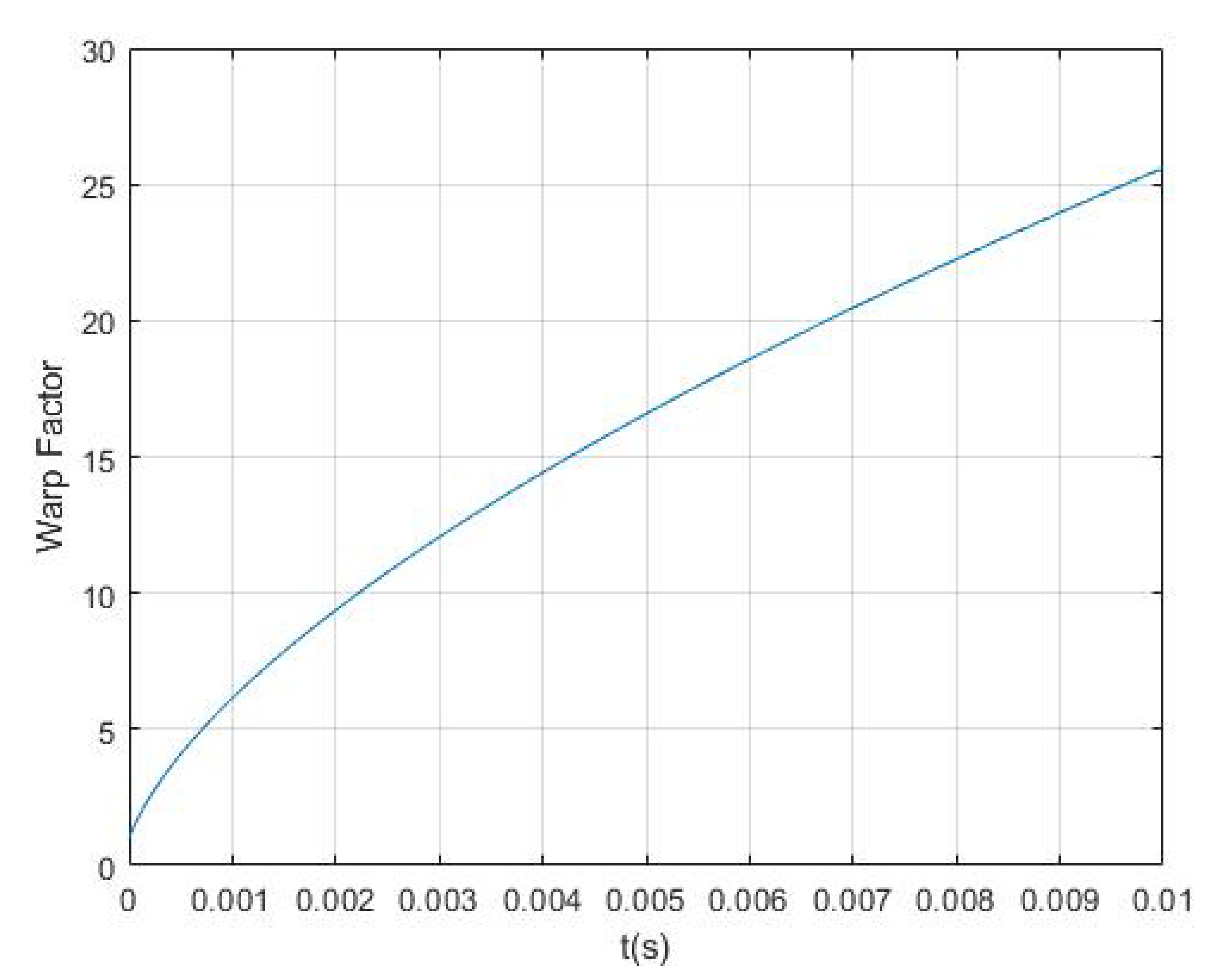
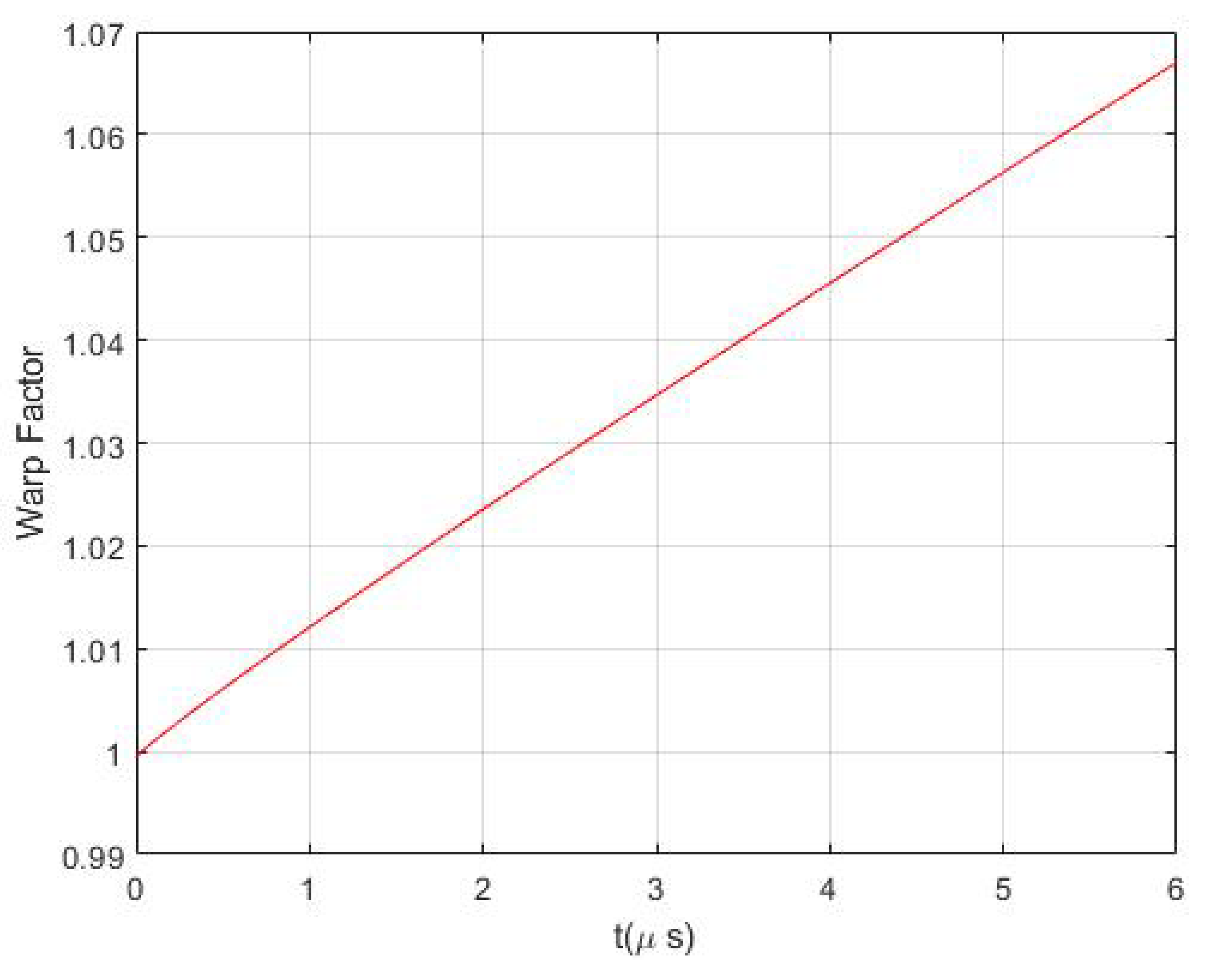
This result is independent of the sphere geometry or the Schwarzschild radius. Such a perturbation is not completely physical. Thus, we considered some others with the characteristic of being practically realizable. Considering the interior solution, for a perturbation like ${\alpha }_1=A{t}^2$, we obtain Figure 1 and for a sinusoidal perturbation we get Figure 2.

As expected from the toy model, the warp factor is always greater than one and can reach significantly large values depending on the applied perturbation.

7. Conclusions

We have solved the Einstein equations for a strong perturbation in the case of a spherical symmetry solution. In this case, the perturbation series reduces to the case of a gradient expansion and the equations are amenable to an exact analytical treatment. We were able to show that, when a perturbation is properly applied, there appears a multiplicative warp factor on the radial velocity that can, in this way, increase exponentially in time. This warp effect does not require significant energy and everything is completely in the realm of positive energy solutions of the Einstein equations, even if as a perturbation series.

We hope these results will find some application in the near future.

References

- Cook, G.; Teukolsky, S. Numerical relativity: Challenges for computational science. Acta Numer. 1999, 8, 1–45. [Google Scholar] [CrossRef] [Green Version]
- Frasca, M. Strong coupling expansion for general relativity. Int. J. Mod. Phys. D 2006, 15, 1373–1386. [Google Scholar] [CrossRef] [Green Version]
- Kalathnikov, I.M.; Lifshitz, E.M. General Cosmological Solution of the Gravitational Equations with a Singularity in Time. Phys. Rev. Lett. 1970, 24, 76–79. [Google Scholar] [CrossRef]
- Belinsky, V.A.; Kalathnikov, I.M.; Lifshitz, E.M. Oscillatory approach to a singular point in the relativistic cosmology. Adv. Phys. 1970, 19, 525–573. [Google Scholar] [CrossRef]
- Belinsky, V.A.; Kalathnikov, I.M.; Lifshitz, E.M. A General Solution of the Einstein Equations with a Time Singularity. Adv. Phys. 1982, 31, 639–667. [Google Scholar] [CrossRef]
- Alcubierre, M. The Warp drive: Hyperfast travel within general relativity. Class. Quant. Grav. 1994, 11, L73–L77. [Google Scholar] [CrossRef]
- Santos-Pereira, O.L.; Abreu, E.M.C.; Ribeiro, M.B. Dust content solutions for the Alcubierre warp drive spacetime. Eur. Phys. J. C 2020, 80, 786. [Google Scholar] [CrossRef]
- Lentz, E.W. Breaking the Warp Barrier: Hyper-Fast Solitons in Einstein-Maxwell-Plasma Theory. arXiv 2020, arXiv:2006.07125. [Google Scholar]
- Teitelboim, C. The Hamiltonian structure of two-dimensional space-time and its relation with the conformal anomaly. In Quantum Theory of Gravity; Christensen, S., Ed.; Adam Hilger: Bristol, UK, 1984; pp. 327–344. [Google Scholar]
- Jackiw, R. Liouville field theory: A two-dimensional model for gravity. In Quantum Theory of Gravity; Christensen, S., Ed.; Adam Hilger: Bristol, UK, 1984; pp. 403–420. [Google Scholar]
- D’Hoker, E.; Jackiw, R. Liouville Field Theory. Phys. Rev. D 1982, 26, 3517–3542. [Google Scholar] [CrossRef]
- Frasca, M. Duality in perturbation theory. Phys. Rev. A 1998, 58, 3439–3442. [Google Scholar] [CrossRef] [Green Version]
- Soffel, M.H.; Han, W.B. Applied General Relativity; Springer: Berlin/Heidelberg, Germany, 2019. [Google Scholar]
- Merritt, D.; Milosavljevic, M. Massive black hole binary evolution. Living Rev. Rel. 2005, 8, 8. [Google Scholar] [CrossRef]
Figure 1.
Warp factor for a perturbation with an equation of motion .
Figure 2.
Warp factor for a perturbation with frequency 1 MHz and equation of motion .
Publisher’s Note: MDPI stays neutral with regard to jurisdictional claims in published maps and institutional affiliations. |
© 2020 by the authors. Licensee MDPI, Basel, Switzerland. This article is an open access article distributed under the terms and conditions of the Creative Commons Attribution (CC BY) license (http://creativecommons.org/licenses/by/4.0/).
Share and Cite
MDPI and ACS Style
Frasca, M.; Liberati, R.M.; Rossi, M. Warping Effects in Strongly Perturbed Metrics. Physics 2020, 2, 665-678. https://0-doi-org.brum.beds.ac.uk/10.3390/physics2040039
AMA Style
Frasca M, Liberati RM, Rossi M. Warping Effects in Strongly Perturbed Metrics. Physics. 2020; 2(4):665-678. https://0-doi-org.brum.beds.ac.uk/10.3390/physics2040039
Chicago/Turabian StyleFrasca, Marco, Riccardo Maria Liberati, and Massimiliano Rossi. 2020. "Warping Effects in Strongly Perturbed Metrics" Physics 2, no. 4: 665-678. https://0-doi-org.brum.beds.ac.uk/10.3390/physics2040039