Dynamics of a Homogeneous and Isotropic Space in Pure Cubic f(R) Gravity


National Research Nuclear University MEPhI (Moscow Engineering Physics Institute), Kashirskoe Shosse 31, 115409 Moscow, Russia
Physics 2021, 3(2), 379-385; https://0-doi-org.brum.beds.ac.uk/10.3390/physics3020027
Submission received: 22 March 2021
/
Revised: 29 April 2021
/
Accepted: 5 May 2021
/
Published: 18 May 2021
(This article belongs to the Special Issue Beyond the Standard Models of Physics and Cosmology)
Abstract
:The possible ways of dynamics of a homogeneous and isotropic space described by the Friedmann–Lemaitre–Robertson–Walker metric in the framework of cubic in the Ricci scalar gravity in the absence of matter are considered. This paper points towards an effective method for limiting the parameters of extended gravity models. A method for -gravity models, based on the metric dynamics of various model parameters in the simplest example is proposed. The influence of the parameters and initial conditions on further dynamics are discussed. The parameters can be limited by (i) slow growth of space, (ii) instability and (iii) divergence with the inflationary scenario.
1. Introduction
Despite the success of experimental tests of the theory of general relativity (GR) with excellent accuracy [1,2,3], the study of various modifications of the theory of gravity continues to date. Historically, the first attempts at modifying GR were aimed towards the unification of gravity with other interactions by adding higher dimensions [4,5]. Modern interest in modified gravity has increased with the emergence of a large set of observational cosmology data [6]. The rapid development of experimental cosmology has cast doubt on the Big Bang theory. The standard cosmology of the Big Bang was described in the framework of GR. In the case of a homogeneous and isotropic space, Einstein’s equations lead to the Friedmann solutions [7], which describe the stages of dominance of radiation and matter. However, modern observational data indicate the existence of stages of accelerated expansion of the universe. The first is the inflation hypothesis, which is not only required to solve flatness and horizon problems, but also to explain the nearly flat temperature anisotropy spectrum observed in the cosmic microwave background [8]. The second is the modern accelerated expansion stage [9,10]. These two stages of the accelerated expansion of the universe can not be explained in terms of standard matter with the known equation of state in the framework of GR. However, these phenomena can be explained in the framework of modified gravity.
One of the simplest approaches to modified gravity is gravity, with being function of the Ricci scalar R. This class of theories is widely used in modern research [11,12,13,14] and, in some cases, successfully solves particular problems and fits the observational cosmology data [15,16,17,18]. The first one and most successful formulation belonging to the class of theories was the Starobinsky model [19] containing only one free parameter. In this model, the addition of the –term was made for elimination of cosmological singularity and led to the inflationary stage. The Starobinsky’s inflationary model is a particular solution to the class of theories of gravity with higher derivatives, which are devoid of ghost degrees of freedom, perturbatively unitary and finite at the quantum level [20]. This model has a “graceful exit” from inflation and provides a mechanism for the subsequent creation and final thermalization of the standard matter. However, adding a cubic term may provide a better agreement with inflationary data, as was recently shown in [21].
In this paper, a way of studying the possible ways of evolution of a homogeneous and isotropic space in the framework of cubic gravity is proposed. Considering only the gravitational component of the evolution, the influence of parameters and initial conditions on further dynamics are discussed.
2. Basic Equations
Let us consider the theory with the following action:
The rationalized Planck units are used where ℏ is the reduced Planck constant, is the Boltzmann constant, c is the speed of light, and G is the Newtonian gravitational constant. Hence, the Planck mass . is the metric tensor with the metric signature . The indices denoted by Greek letters take on the values .
By varying this action with respect to the metric and using conventions for the curvature tensor as and the Ricci tensor is , we obtain the equation of motion for the gravity theory
Here, , and .
Considering the metrics of homogeneous and isotropic spaces, namely,
corresponding to spaces with positive (3), zero (4) and negative (5) curvatures, from Equations (2), one obtains the nontrivial following equations:
where the Ricci scalar for the metrics used is
with for metric (3), for metric (4) and for metric (5). The dot denotes the time derivative .
In order to find a solution, a system to be determined, consisting of Equation (7) and the definition the Ricci scalar, Equation (8). Equation (6) to be used as a constraint on the initial condition.
Let us choose the initial conditions for the unknown functions and of the system of Equations (7) and (8) as
and then the initial value of the curvature to be obtained by solving Equation (6).
The choice of the initial conditions is the most difficult task. In the formulation of the problem used here, the conditions (9) are free parameters that one introduces“by hand”. In addition to the problem of choosing the initial conditions, some models contain the possibility of several asymptotic values of the Ricci scalar for a particular form of the function. Here, the simplest case when the chosen function has the form,
is considred. In this case, the trace of Equations (2) at the constant curvature, , leads to
which defines the asymptotic values of the Ricci scalar. For the simplest case, when more than one asymptotic value is possible, from Equation (11), one obtains:
So what conditions lead to the realization of a particular asymptotics?
3. Analysis in the Einstein Frame
In this Section, the effect of the model parameter values and initial conditions on the dynamics of the spaces are verified. The action (1) can be reduced to scalar-tensor (ST) theory by introducing an auxiliary scalar field as a result of the Legendre transformation [22]:
where . Upon conformal transformation, one obtains this action in the Einstein (E) frame:
where the new variables are introduced, namely,
To avoid the antigravity regime, the condition [23], is set. One of the classical equations of the action (13) is and, then, if . Using the form (15) of the potential , a condition,
for a local extremum of an auxiliary scalar field can be found. The condition (16) is exactly the condition (11) obtained above, which leads to a de Sitter space endowed with constant curvature.
The existence of a stable minimum for a scalar field then follows from
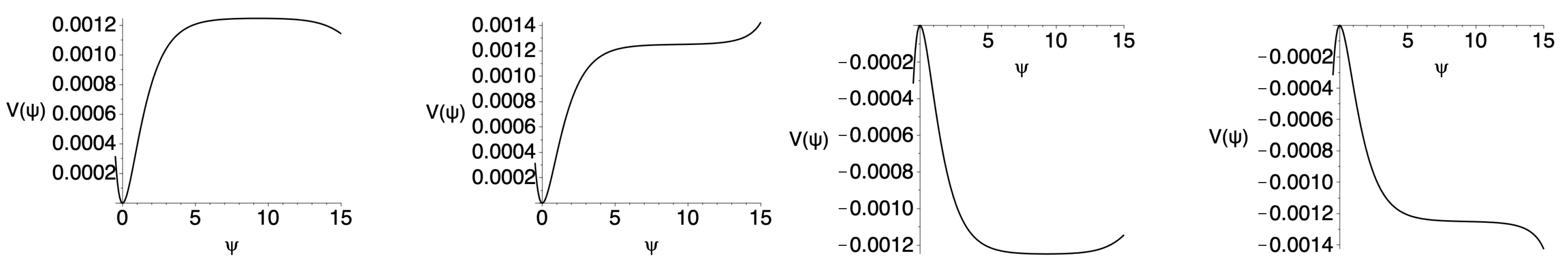
From the condition (17) one gets for chosen form (10),
One of the asymptotics corresponds to the maximum of the potential, while the other one corresponds to its minimum depending on the values of the parameters of the function (10). The potential is shown in Figure 1 for different signs of the parameters of the function (10). It should be noted that the introduced value of is related to the auxiliary scalar field by Equation (15) with .
An unstable position is possible at large values in the far left and far right plots of Figure 1, where both coefficients and have the same sign. The initial conditions in situation at the far left plot can play an important role leading to an unstable solution. The chosen initial conditions (9) and values of the coefficients must lead to a value to ensure the stability of the solution. Instability in the far right plot arises regardless of the choice of initial conditions. The dynamics for the other two cases of the parameters values, as shown in the second and third plots of Figure 1, are quite predictable. Regardless of the initial value of the curvature, the solutions will tend to and then reach a stable minimum.
Thus, the influence of the values of the parameters of the function (10) is revealed determining the implementation of the asymptotics (12). The only exception in the model (10) is the case of the far left picture, where the initial conditions can lead to unstable solutions. The obtained statements be confirmed by numerical calculations in the what follows.
4. Numerical Results
Let us illustrate what was discussed above with the example of a numerical solution for a flat space (4). As it is said in Section 2, a system of Equations (7) and (8) to be solved under the initial conditions (9), chosen near the sub-Planck scale,
where , and the initial value of the curvature to be found by solving Equation (6).
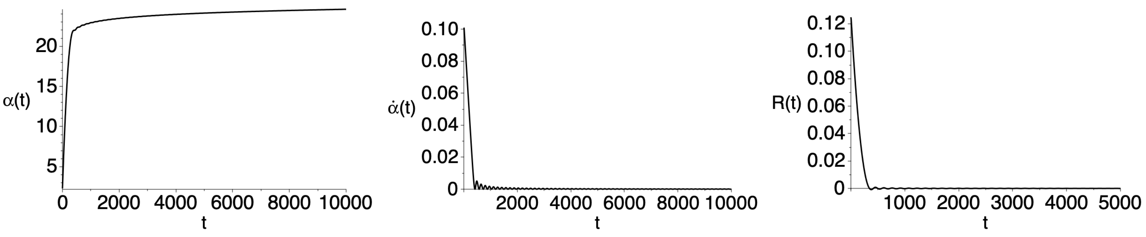
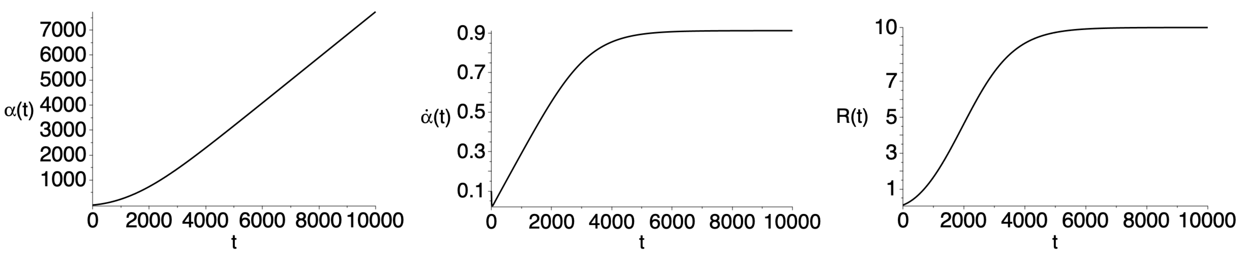
The results of the numerical solution for this Cauchy-type problem are shown in Figure 2 and Figure 3 using the rationalized Planck units. Figure 2 corresponds to the case of the far left plot of Figure 1, and Figure 3 corresponds to the third plot of Figure 1.
In Figure 2, the numerical solution covers several stages of the evolution of the universe. The first is the inflationary stage, where space grows exponentially and the curvature of space decreases. Then, having reached zero, the curvature starts to oscillate around zero and the Hubble parameter, i.e., , at this stage, asymptotically reaches zero, and the size of the space, , tends to a constant. After the damping of the oscillations of the corresponding quantities, a transitional regime begins to the GR. However, the space does not expand enough to describe the visible part of the universe. The value must be , where corresponds to the horizon scale cm at the present time. In addition to the final size of space, one can see that the exponential expansion of space ends earlier than the corresponding duration of the inflationary stage. The exponential expansion of space must continue during (in the rationalized Planck units). During this time, the function must change by the value .
In Figure 3, the space starts its evolution in the early stage in a similar way, but then enters a different asymptotic behavior which is defined by the signs of the coefficients and does not correspond to the observable universe. As a result, one obtains an infinitely exponentially growing space endowed with significant curvature.
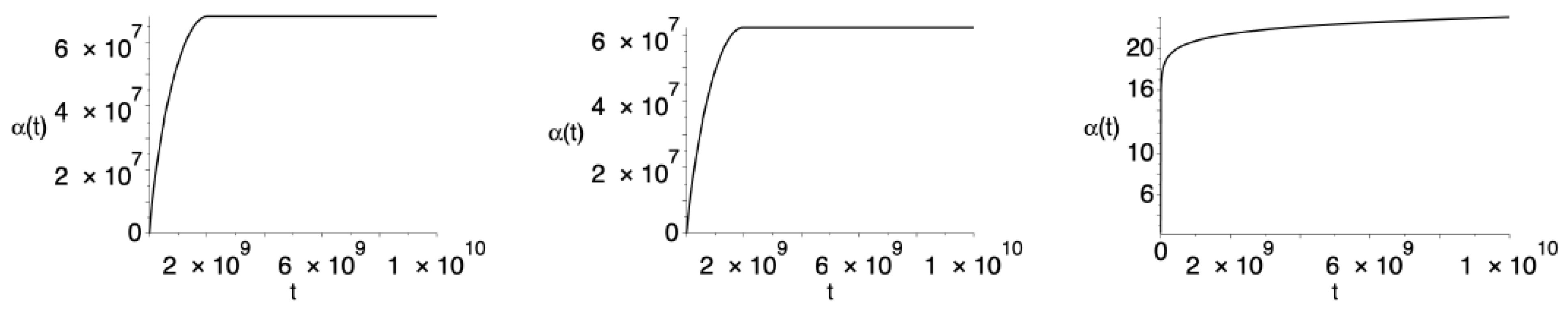
Specific values of the parameters and of the function determine the duration of each stage of evolution and the amplitudes of oscillations that have cosmological significance. In addition to the revealed dependence of the realization of asymptotics on the parameters of the function, the rate of the dynamics of space is also an important issue. The previous reasoning and conclusions in Section 3 did not depend on the particlar choice of the metric. Let us find a numerical solution for three possible configurations of a homogeneous and isotropic spaces (3)–(5). For more realistic results, describing the observable universe, the parameters and , based on the analysis of the inflationary scenario, to be chosen following the constraints from Ref. [21]. The results of the dynamics of spaces of different curvatures with the same choice of parameters and initial conditions (19) are shown in Figure 4.
The obtained results indicate a different rate of dynamics of the spaces. One sees that the behavior of a space with positive curvature (3) and flat space (4) leads to a value of the same order of magnitude in the asymptotics. The dynamics of the space of negative curvature (5) leads to a smaller size than the visible part of the universe.
A similar difference in the rate of expansion of space takes place in the framework of the Starobinsky model [19], namely
5. Discussion
Considering only the gravitational dynamics of a homogeneous and isotropic space, allows us to come to restrictions on function. The asymptotics in case of cubic function are strictly determined by the signs and values of the coefficients. Nevertheless, the choice of the initial conditions can affect the stability of the solution. In addition to the correct asymptotic value of the curvature, it is also worth considering the possible size of space, no less than the size of the visible part of the universe and the values of cosmological parameters available from the observational data [6]. A detailed analysis of cubic gravity in the inflationary scenario was recently performed in [21]. It was shown that an extension of Starobinsky’s model allows for better agreement with experimental data. However, considering the purely gravitational dynamics of an isotropic and homogeneous space [24] the acceptable range of values of the coefficients of function has an intersection with the range of values from [21], less than each of them provides separately.
Besides, at Planck energy scales, fluctuations can lead to the formation of asymmetric spaces. The description of this process can be done only by the theory of quantum gravity, which has not yet been developed. The spaces of different curvatures have different rates of expansion as a result of our numerical solutions of the classical equations of motion. Then, can our Universe be homogeneous and have isotropic space outside the visible part? This issue will be discussed in future studies.
Funding
This research received no external funding.
Institutional Review Board Statement
Not applicable.
Informed Consent Statement
Not applicable.
Data Availability Statement
Not applicable.
Acknowledgments
I would like to thank Sergey G. Rubin for the usefull discussions and interest to the work. The work was supported by the Ministry of Science and Higher Education of the Russian Federation, Project “Fundamental properties of elementary particles and cosmology” No 0723-2020-0041. This work was as part of the course “Cosmoparticle physics” in National Research Nuclear University MEPhI.
Conflicts of Interest
The authors declare no conflict of interest.
References
- Yunes, N.; Siemens, X. Gravitational-wave tests of general relativity with ground-based detectors and pulsar-timing arrays. Living Rev. Relativ. 2013, 16, 9. [Google Scholar] [CrossRef] [PubMed] [Green Version]
- Will, C.M. The confrontation between general relativity and experiment. Living Rev. Relativ. 2014, 17, 4. [Google Scholar] [CrossRef] [Green Version]
- Berti, E.; Barausse, E.; Cardoso, V.; Gualtieri, L.; Pani, P.; Sperhake, U.; Zilhao, M. Testing general relativity with present and future astrophysical observations. Class. Quantum Gravity 2015, 32, 243001. [Google Scholar] [CrossRef]
- Kaluza, T. Zum Unitätsproblem der Physik. Sitzungsber. K. Preuss. Akad. Wiss. (Berl.) 1921, 966–972. English translation: Kaluza, T. On the unification problem in physics. Int. J. Mod. Phys. D 2018, 27, 1870001. [Google Scholar] [CrossRef]
- Klein, O. The Atomicity of electricity as a quantum theory law. Nature 1926, 118, 2971. [Google Scholar] [CrossRef]
- Planck Collaboration; Aghanim, N.; Akrami, Y.; Ashdown, M.; Aumont, J.; Baccigalupi, C.; Ballardini, M.; Roudier, G. Planck 2018 results. VI. Cosmological parameters. Astron. Astrophys. 2020, 641, A6. [Google Scholar] [CrossRef] [Green Version]
- Friedman, A. Über die Krümung des Raumes. Z. Phys. 1922, 10, 377–386. [Google Scholar] [CrossRef]
- Planck Collaboration; Akrami, Y.; Ashdown, M.; Aumont, J.; Baccigalupi, C.; Ballardini, M.; Banday, A.J.; Barreiro, R.B.; Bartolo, N.; Basak, S. Planck 2018 results. VII. Isotropy and statistics of the CMB. Astron. Astrophys. 2020, 641, A7. [Google Scholar] [CrossRef] [Green Version]
- Riess, A.G.; Filippenko, A.V.; Challis, P.; Clocchiatti, A.; Diercks, A.; Garnavich, P.M.; Gilliland, R.L. Observational evidence from supernovae for an accelerating universe and a cosmological constant. Astron. J. 1998, 116, 1009. [Google Scholar] [CrossRef] [Green Version]
- Perlmutter, S.; Aldering, G.; Goldhaber, G.; Knop, R.A.; Nugent, P.; Castro, P.G.; Deustua, S. Measurements of Ω and Λ from 42 high-redshift supernovae. Astrophys. J. 1999, 517, 565. [Google Scholar] [CrossRef]
- De Felice, A.; Tsujikawa, S. f(R) theories. Living Rev. Relativ. 2010, 13, 3. [Google Scholar] [CrossRef] [Green Version]
- Capozziello, S.; de Laurentis, M. Extended theories of gravity. Phys. Rep. 2011, 509, 167–321. [Google Scholar] [CrossRef] [Green Version]
- de la Cruz-Dombriz, A.; Saez-Gomez, D. Black holes, cosmological solutions, future singularities and their thermodynamical properties in modified gravity theories. Entropy 2012, 14, 1717–1770. [Google Scholar] [CrossRef]
- Nojiri, S.; Odintsov, S.D. Unified cosmic history in modified gravity: From F(R) theory to Lorentz non-invariant models. Phys. Rep. 2011, 505, 59–144. [Google Scholar] [CrossRef] [Green Version]
- Starobinsky, A.A. Disappearing cosmological constant in f(R) gravity. J. Exp. Ther. Phys. Lett. 2007, 86, 157–163. [Google Scholar] [CrossRef] [Green Version]
- Tsujikawa, S. Observational signatures of f(R) dark energy models that satisfy cosmological and local gravity constraints. Phys. Rev. D. 2008, 77, 023507. [Google Scholar] [CrossRef] [Green Version]
- Nojiri, S.; Odintsov, S.D.; Saez-Gomez, D. Cosmological reconstruction of realistic modified F(R) gravities. Phys. Lett. B 2009, 681, 74–80. [Google Scholar] [CrossRef] [Green Version]
- Nojiri, S.; Odintsov, S.D.; Oikonomou, V.K. Unifying inflation with early and late-time dark energy in F(R) gravity. Phys. Dark Univ. 2020, 29, 100602. [Google Scholar] [CrossRef]
- Starobinsky, A.A. A new type of isotropic cosmological models without singularity. Phys. Lett. B 1980, 91, 99–102. [Google Scholar] [CrossRef]
- Koshelev, A.S.; Modesto, L.; Rachwal, L.; Starobinsky, A.A. Occurrence of exact R2 inflation in non-local UV-complete gravity. J. High Energy Phys. 2016, 11, 67. [Google Scholar] [CrossRef] [Green Version]
- Cheong, D.Y.; Lee, H.M.; Park, S.C. Beyond the Starobinsky model for inflation. Phys. Lett. B 2020, 805, 135453. [Google Scholar] [CrossRef]
- Rubin, S.G.; Popov, A.; Petriakova, P.M. Gravity with higher derivatives in D-dimensions. Universe 2020, 6, 187. [Google Scholar] [CrossRef]
- Nojiri, S.; Odintsov, S.D. Modified gravity with negative and positive powers of curvature: Unification of inflation and cosmic acceleration. Phys. Rev. D 2003, 68, 123512. [Google Scholar] [CrossRef] [Green Version]
- Petriakova, P.; Popov, A.; Rubin, S. Sub-Planckian scale and limits for f(R) models. Symmetry 2021, 13, 313. [Google Scholar] [CrossRef]
Figure 1.
The potential (15) for different values of the parameters of the function (10): , (first); , (second); , (third) and , (last).

Figure 2.
The solution of the system of Equations (7) and (8) with parameters , with the initial conditions , , and . The asymptotic behavior is and the Hubble parameter . The parameter values and correspond to the leftmost plot in Figure 1. The rationalized Planck units are used, so the Planck mass, .

Figure 3.
The solution of the system of Equations (7) and (8) with parameters , and initial conditions , , and . The asymptotic behavior is and the Hubble parameter . The parameter values and correspond to the third plot in Figure 1. The rationalized Planck units are used, so the Planck mass, .

Figure 4.
The solution of the system of Equations (7) and (8) with parameters , and initial conditions , and for the metric (3) (first), (4) (second) and (5) (third), for each case, defined from the solution to Equation (6). The rationalized Planck units are used, hence, the Planck mass, .


Publisher’s Note: MDPI stays neutral with regard to jurisdictional claims in published maps and institutional affiliations. |
© 2021 by the author. Licensee MDPI, Basel, Switzerland. This article is an open access article distributed under the terms and conditions of the Creative Commons Attribution (CC BY) license (https://creativecommons.org/licenses/by/4.0/).
Share and Cite
MDPI and ACS Style
Petriakova, P. Dynamics of a Homogeneous and Isotropic Space in Pure Cubic f(R) Gravity. Physics 2021, 3, 379-385. https://0-doi-org.brum.beds.ac.uk/10.3390/physics3020027
AMA Style
Petriakova P. Dynamics of a Homogeneous and Isotropic Space in Pure Cubic f(R) Gravity. Physics. 2021; 3(2):379-385. https://0-doi-org.brum.beds.ac.uk/10.3390/physics3020027
Chicago/Turabian StylePetriakova, Polina. 2021. "Dynamics of a Homogeneous and Isotropic Space in Pure Cubic f(R) Gravity" Physics 3, no. 2: 379-385. https://0-doi-org.brum.beds.ac.uk/10.3390/physics3020027