
SIR-PID: A Proportional–Integral–Derivative Controller for COVID-19 Outbreak Containment


Laboratori Nazionali del Gran Sasso, Istituto Nazionale di Fisica Nucleare, Via G. Acitelli, 22, Assergi, 67100 L’Aquila, Italy
*
Author to whom correspondence should be addressed.
Physics 2021, 3(3), 459-472; https://0-doi-org.brum.beds.ac.uk/10.3390/physics3030031
Submission received: 25 April 2021
/
Revised: 9 June 2021
/
Accepted: 11 June 2021
/
Published: 27 June 2021
(This article belongs to the Special Issue Physics Methods in Coronavirus Pandemic Analysis)
Abstract
:Ongoing social restrictions, including social distancing and lockdown, adopted by many countries to inhibit spread of the the COVID-19 epidemic, must attempt to find a trade-off between induced economic damage, healthcare system collapse, and the costs in terms of human lives. Applying and removing restrictions on a system with a given latency as represented by an epidemic outbreak (and formally comparable with mechanical inertia), may create critical instabilities, overshoots, and strong oscillations in the number of infected people around the desirable set-point, defined in a practical way as the maximum number of hospitalizations acceptable by a given healthcare system. A good understanding of the system reaction to any change of the input control variable can be reasonably achieved using a proportional–integral–derivative controller (PID), which is a widely used technique in various physics and technological applications. In this paper, this control theory to is proposed to be applied epidemiology, to understand the reaction of COVID-19 propagation to social restrictions and to reduce epidemic damages through the correct tuning of the containment policy. Regarding the synthesis of this interdisciplinary approach, the extended to the susceptible–infectious–recovered (SIR) model name “SIR-PID” is suggested.
1. Introduction
The diffusion of the coronavirus disease (COVID-19) outbreak, caused by severe acute respiratory syndrome coronavirus 2 (SARS-CoV-2) [1,2], is described, as for typical epidemics, by the so-called basic reproduction number (or ratio), usually denoted [3] and defined as the expected number of new infections from a single new case in a population where all subjects are susceptible.
A sizeable fraction of people infected by COVID-19, especially those who are older and with underlying preexisting medical problems, are likely to develop a serious illness with a fatality rate well above the typical seasonal influenza [4]. To mitigate this problem, many countries have adopted drastic or moderate social restrictions to reduce and control by limiting the population mobility, which determines the interactions among people. In early 2020, due to the lack of data on virus diffusion and transmission dynamics, social distance policies emerged as the main method to mitigate the outbreak [5,6,7].
Another parameter, called the effective reproduction number and labelled as , is also used and accounts for the evolution of in time. However, for the sake of notation simplicity, let us keep one definition in compliance with the standard compartmental models used in epidemiology that is described below.
In this paper, an attempt to study how to manage the diffusion of COVID-19 by exploiting the concept of control loop mechanism, used in physics technologies, is made. This idea is based on the consideration that social restrictions aimed at reducing the diffusion of the virus that, at the same time, imply a negative impact of the pandemic on the economy. Therefore, the need to balance these effects appears obvious. Such an operation is typical of a modulated control mechanism. The use of dynamic control theories has been applied to the diffusion of a virus [8] and to lockdown effects [9] although with a different approach to this study. In those approaches, the optimal lockdown policy, in a mathematical model-dependent framework, is typically chosen to maximize a given social objective as a trade-off between the economic loss and the cost of the epidemic. In this paper, a generalization of those approaches through the integration with a well-known control theory used in physics and engineering is proposed.
As a general consideration, drastic social restrictions, such as the so-called lockdown, cannot last too many weeks because it may cause serious damage to the economy; on the other hand, relaxing too much the epidemic containment in a subsequent phase may cause a restart of the pandemic growth, thus, setting a country into an even more critical status [10]. The best condition would be a compromise in which is brought close to the unity (or, better, ≤1) with the number of active cases reasonably close to a given threshold, represented by the capability of a healthcare system to maximize the number of recovered people and to avoid system collapse. This threshold is reasonably close to the maximum number of available intensive care hospitalizations. This steady condition is meant to be optimal, while waiting for the manufacture and the administration of a vaccine [11].
The problem of manipulating the people’s mobility, and thus trying to change , is, in general, not straightforward for the enormous inertia (resistance to changes) of the epidemic propagation. This is due to two factors that characterize COVID-19, namely the long incubation period or latency (up to 14 days [12]) and the long recovery time (up to or longer than one month). In simple terms, it is not easy to act on a system with such a long latency and fast reaction to relaxation [13,14,15,16]: if one tries to relax the restrictions or wait too long to set them, the effects will be visible only after a certain period. This behaviour is analogous to mechanical inertia.
In fact, one has seen, from the beginning of 2020 to the present, more than a year later, multiple waves of infections that have devastated many countries in a desperate attempt to set restrictions to slow down the pandemic diffusion and, soon after, release them when the situation seemed to have improved. This policy has not been effective: see for example the COVID-19 “new cases” trends of many countries in Europe and/or in America from the beginning of the pandemic to the beginning of the vaccinations [17]. The observed pandemic restriction behaviour can be compared with the typical cases in many technological systems in which a control system attempts to reach a set-point in a smooth way avoiding dangerous stress and unstable oscillations of the system itself.
The control system theory is quite complicated, and different solutions have been studied over the centuries [18]. One fundamental approach, sometimes with some limitations, but in general with high performance, is the proportional–integral–derivative controller (PID) [19]. In this paper, the most important features of this theory are exploited to understand the evolution of the COVID-19 outbreak when controlled with social restrictions. This modelling may help in understanding the COVID-19 evolution in many countries. Its description can be used to choose the right sequence of social restrictions during an epidemic. The novel aspect of the present analysis, which is called “SIR-PID” here, extending the susceptible–infectious–recovered (SIR) model, is the application of a well-established control technology to epidemiology science, with the advantage of gaining a new tool for limiting and controlling the social and economical damage produced by a serious epidemic, such as COVID-19, that is expandable to many epidemiological models and, in principle, will work even without a specific model.
In Section 2, the PID controller theory is introduced with its most important features. In Section 3, a mathematical model for the COVID-19 epidemic evolution is described based on the time-dependent modification of the SIR compartmental model. In Section 4, the numerical implementation of the resulting SIR-PID model is given, proposed as a test-bench model. In Section 5, the tuning of the SIR-PID coefficients is described. Finally, in Section 6, a simple method of implementing the mechanism on real data dealing with large statistical uncertainty is recommended.
2. The PID Controller
A PID controller is a feedback control loop mechanism widely used in technical systems in which a continuously modulated control is required [19]. Even if certain basic properties were grasped a few centuries ago, the first mathematical formalization dates back to the early 1900s [20]. Currently, PID controllers are used in many automatic processes that require high stability and optimization, but they have interesting applications also in understanding complex biological systems [21,22].
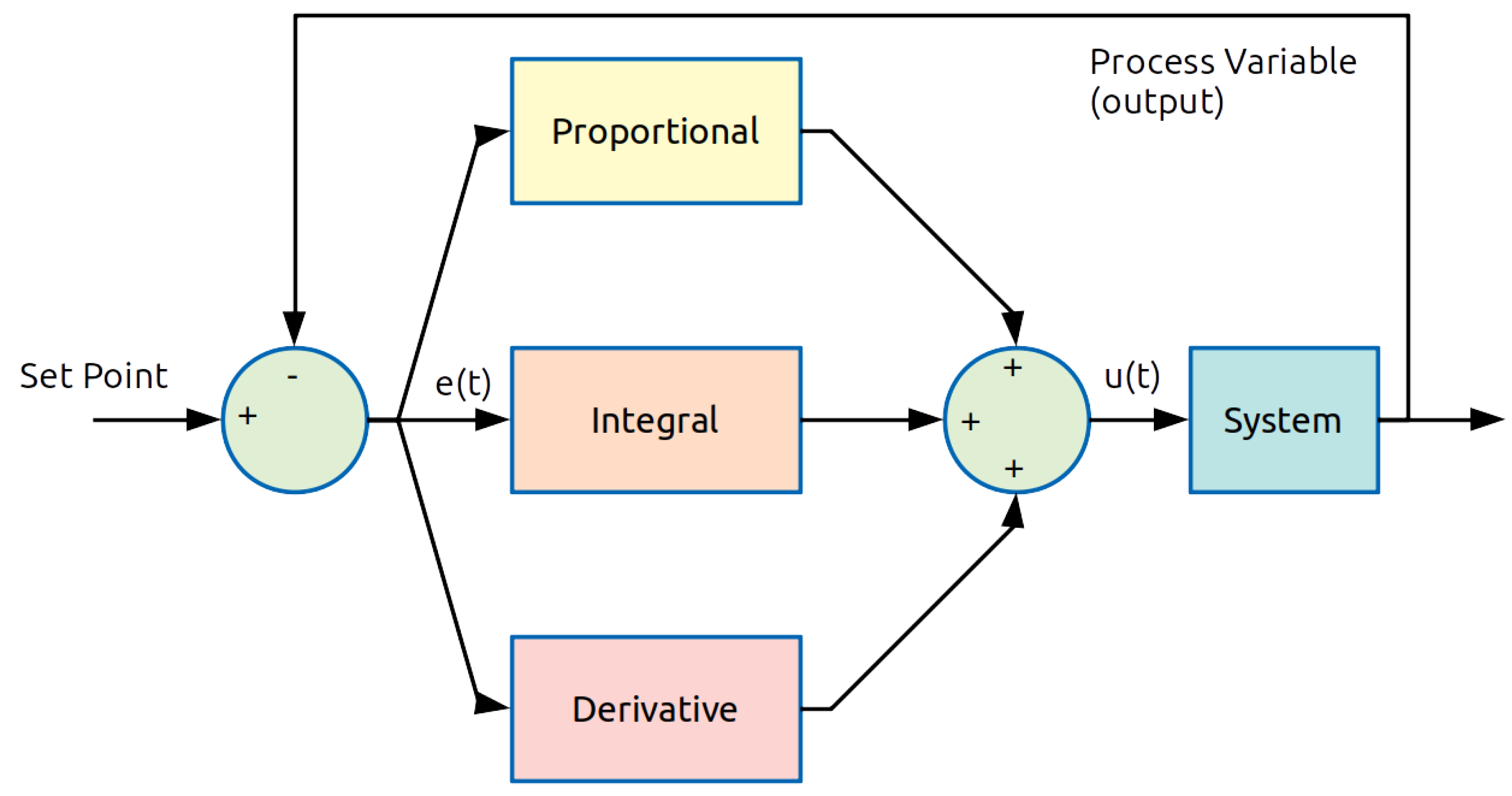
The PID computes on line the time t-dependent error value input, , as the difference between a desired set-point (SP) and a measured process variable (PV), received as feedback. A PID applies correction through the control variable output, , consisting of a weighted average of a proportional (P), integral (I), and derivative (D) terms, according to the flow diagram reported in Figure 1. The controller essentially aims at minimizing the error over time by updating the control variable to a newer value established by control terms. Its explicit mathematical formulation reads:
where , , and represent the proportional, integral, and derivative terms, respectively.
The meaning of the three terms can be summarized as follows. The proportional term represents the action of the present condition of the system and is proportional to through the coefficient . The proportional control alone generates a response only if is different from zero. In other words, if the error is positive, the control output is correspondingly positive and vice versa. The integral term takes into account the past, by adjusting the control output with the cumulative residual error . The integral term stops growing when the set-point is reached, keeping the desired set-point. Finally, the derivative term gives an estimation of the future condition. The control is proportional to the error change rate. Fast change induces fast control and vice versa.
The optimized choice of K’s parameters is achieved after a loop tuning process [23,24]. The values are related to the system response, and they can be tuned with different methods observing the behaviour of the system response after fixing or moving a given set-point. For further detail, see Section 5.
3. The SIR-PID Model
To model the behaviour of the COVID-19 epidemic in the presence of social restrictions aiming at changing the basic reproduction number , let us consider a basic SIR compartmental model [25,26]. This model is modified to account for a time-dependent as described in [27]. Hereafter, this model is referred as SIR-PID. A remark is in order. The basic SIR compartmental model can be expanded to make more elaborate models, such as the one described in [28]. In addition, Monte Carlo methods have also been introduced to enlarge the dynamic of the diffusion taking into account inhomogeneities in the population affected by the virus [29].
In this study, the standard SIR model assumptions are used to exploit the PID feedback method. It is worth noting that, if the system response is known a priori, the control condition can be determined mathematically, independently of the PID mechanism, or one can calculate the PID coefficients a priori. In principle, one can forget this aspect and proceed as if the epidemic system response was completely unknown. This generalizes the specific control to a real epidemic system, such as the COVID-19, i.e., not completely modelled in all its, sometimes unknown, details, giving to the present analysis the potentiality of being applied to model-independent systems.
In the model, three categories of individuals are distinguished, known as compartments: for the number of susceptible, for the number of infectious, and for the number of recovered, or better removed. The last category might include recovered and deceased individuals together or separately. Based on these assumptions, the mathematical model is written in terms of the following set of differential equations:
where is the recovery rate, and is a constant defined with its derivative being equal to zero. In order to match the standard SIR model, corresponds to , usually called the transition rate.
If a susceptible population of people is affected for the first time by the disease outbreak, the initial conditions of the system (2) can be easily cast as: , , and . In the basic SIR model, as reported above, determines the dynamic of the infection, and emerges as the ratio . With this definition, let us focus on the second equation in system (2). From this equation it follows: if . Therefore, the epidemic decreases when .
4. SIR-PID Numerical Implementation
In order to implement and study a simple SIR-PID model, let us group the standard compartment functions , , and in a vector . The system (2) can be easily recast as
with the initial condition: , where represents the nonlinear vectorial function defined in the SIR equations (see the three equations in system (2)).
The system can be solved numerically using e.g., the Runge–Kutta method [30,31] even if, for the sake of simplicity, one considers a simple forward Euler’s method [32]. The latter states that, for each constant iteration , the solution of the differential equation can be incremented as:
In particular, the second component of , representing the infected people or active cases,
is the output of the PID controller, while is the input control variable, where is a normalization constant, that can be chosen equal to one for having a 100% increment at . Defining the error (with e.g., to normalize the response), the SIR-PID model is then implemented as
The second and third terms of the right-hand side represent the numerical approximation of the integral and the derivative of the error , respectively. Finally, let us put some reasonable ingredients in the model:
(i) Let be the typical population of a small country or region. To understand the SIR-PID response, N must be greater than the typical infected population, to avoid the so-called herd immunity turning point, as expected for the free evolution of epidemics without any attempt of containment.
(ii) One can imagine that the outbreak starts with an out-of-control patient zero. The initial condition is, therefore, .
(iii) can range from 0.5 to 10. Let us assume that a country cannot do a total lockdown (), as some basic goods and services must be guaranteed. represents, in this case, the maximum reproduction number, corresponding to the absence of restriction by governments and/or by freedom of action of citizens. This value is assumed as the starting condition for the control variable.
(iv) Social restrictions are applied by the government through official orders every two weeks ( days, the typical time of the virus latency) and, after application, decreases anyway by the inertia of one unit per day. In other words, when a new law restricts people’s mobility, it may take some time to obtain the result, because people need time to become used to the new recommended behaviours. This explains the choice in the modelling made here.
(v) Let the set-point be , representing a threshold chosen in order to not make the healthcare system collapse and guarantee a certain number of intensive care patients.
(vi) Let us choose assuming one month for the typical recovery time.
(vii) Finally, to guarantee good accuracy of the solutions of Equation (3) with the forward Euler’s method, let us set day.
The system is free to evolve and ready for tuning.
5. Tuning and Interpretation
The tuning process aims at the best calibration of the proportional gain, the integral gain, and the derivative correction to select the proper proportional bands. The final goal is to reach system stability within the desired range with the desired time scale. The PID tuning is a quite complex problem because each system has a different (very often unknown) response, even if the selection of the P, I, and D parameters may look quite intuitive.
Many different procedures have been developed over the years. Some empirical rules, such as Ziegler–Nichols tuning [33], appear quite flexible and usable for the majority of the technological applications. It is also possible to determine the PID coefficients performing complex system simulations, and there are many algorithms of self-tuning. For further details, see e.g., [34].
In summary, the tuning can be a manual process based on experience, a methodical process based on known rules, an automatic process based on software, or a combination of them. Manual tunings can be time-consuming and can damage the system if the reaction is completely unknown, while a tuning based on rules, as Ziegler–Nichols, is faster and safer, even if it cannot be applied to all systems. Conversely, an automatic tuning based on software tools can identify the system model from test samples of data and model the PID controller with specific algorithms.
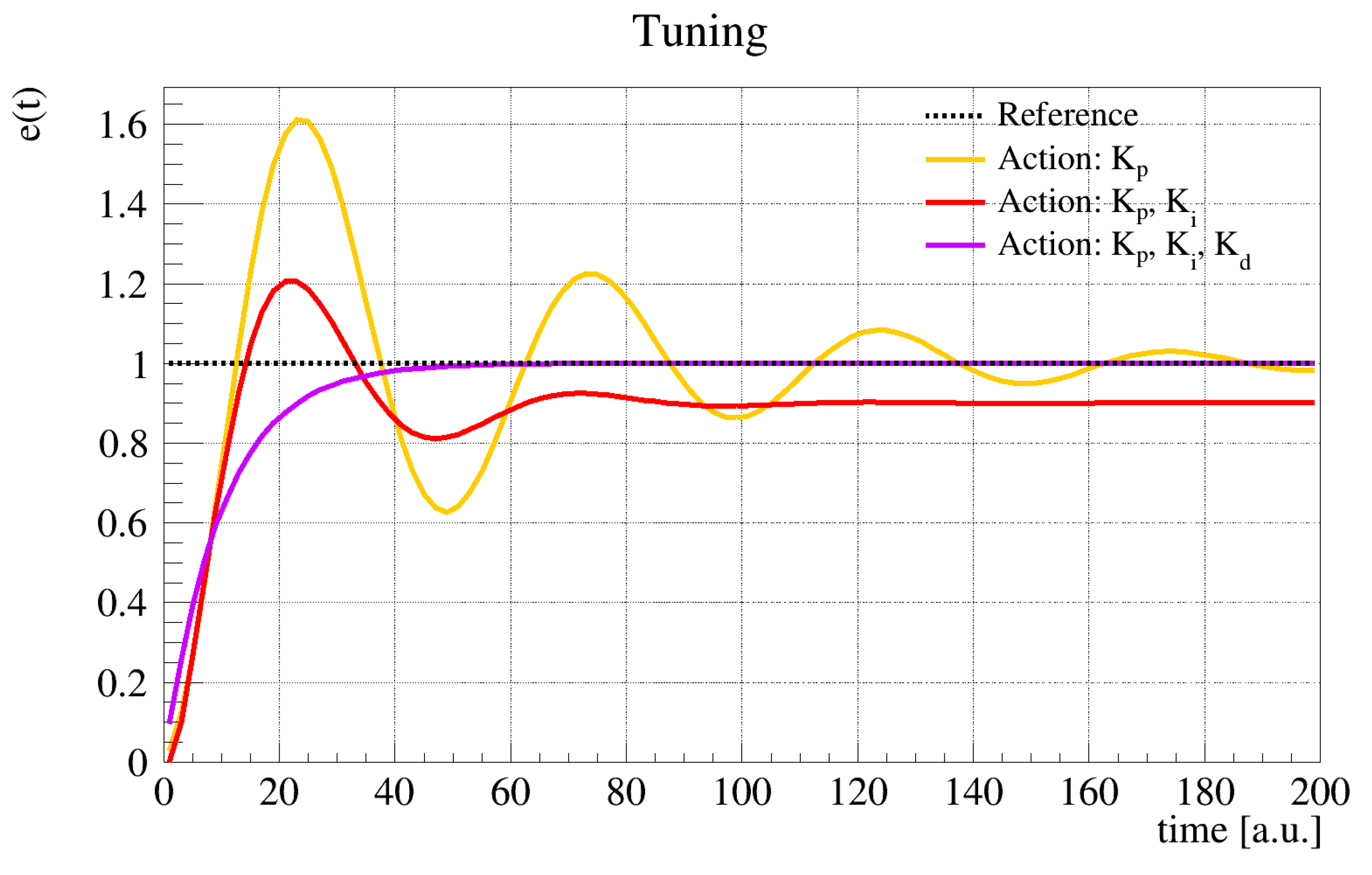
To have an idea of a tuning process, let us consider a manual approach. The starting point is setting with increasing only the process until the output starts oscillating. At this point, can be almost halved, and the user can start increasing (to compensate the offset with respect to the set-point) and (to react to the fast changes and damping, a possible ringing around the off-set). An example reported in Figure 3 shows the contribution of the different terms during manual tuning. In particular, Figure 3 shows a generic system responding respectively to a pure proportional control (red), a proportional corrected with the integral term (yellow) for removing the bias with the set-point (dashed black), and finally with oscillation damped by the derivative term (violet).
Following a manual tuning, the different behaviours of the SIR-PID is reported below when introducing step by step different values for the PID coefficients.
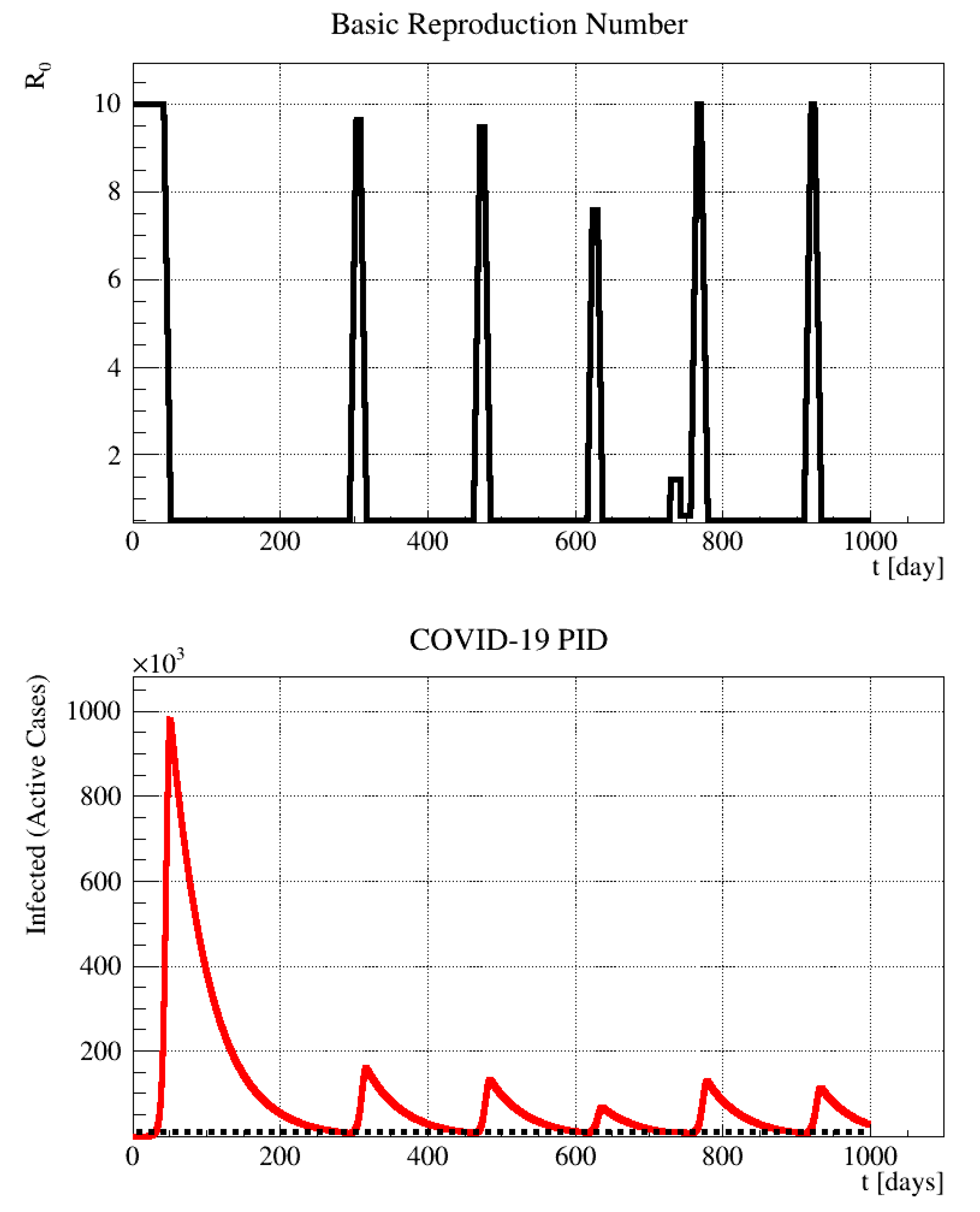
Figure 4 shows the behaviour of input (top) and output bottom with , . The dashed black line represents the set-point. A very strong proportional action only was not able to stabilize the system. This corresponds to the complete absence of restrictions at the beginning and a drastic lockdown when the threshold is reached, and this behaviour was repeated every time the set-point was reached, causing many out-of-control devastating epidemic waves. This scenario could happen when excessive optimism makes the restrictions relax too early until the situation becomes out-of-control again and another drastic lockdown is needed. Such behaviour has been seen in many countries since the beginning of 2020.
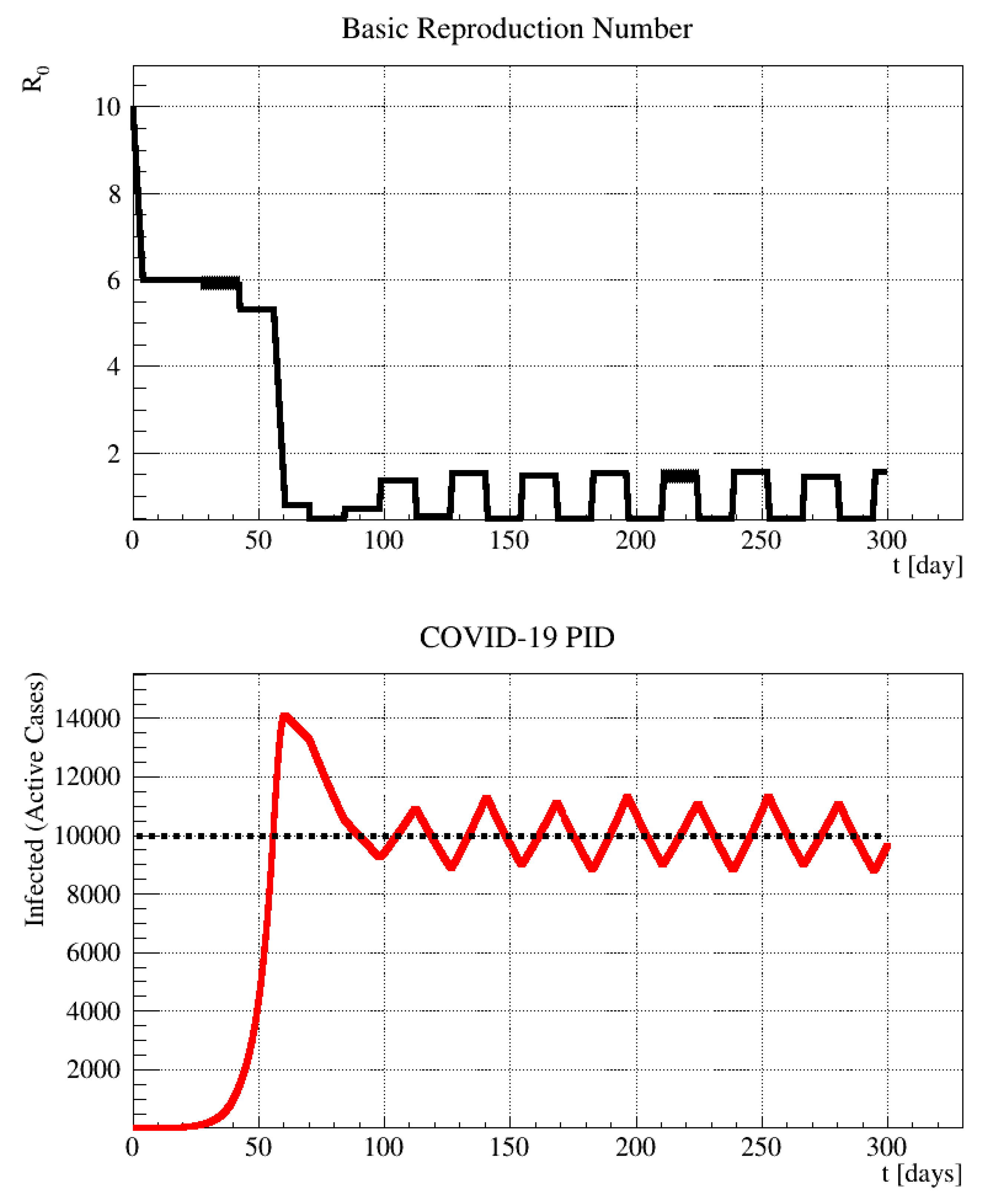
In Figure 5, the behaviour of input (top) and output (bottom) with and is shown. A milder proportional term avoids a strong overshoot at the first reach of the set-point but is not sufficient for damping the system oscillation. This corresponds to a less drastic social restriction at the beginning and then a subsequent attempt to stabilize the rate with a mild and strong lockdown. This situation could be, in principle acceptable, yet the residual oscillations can create instabilities and make people unhappy with the continuous changes of the restrictions policy.
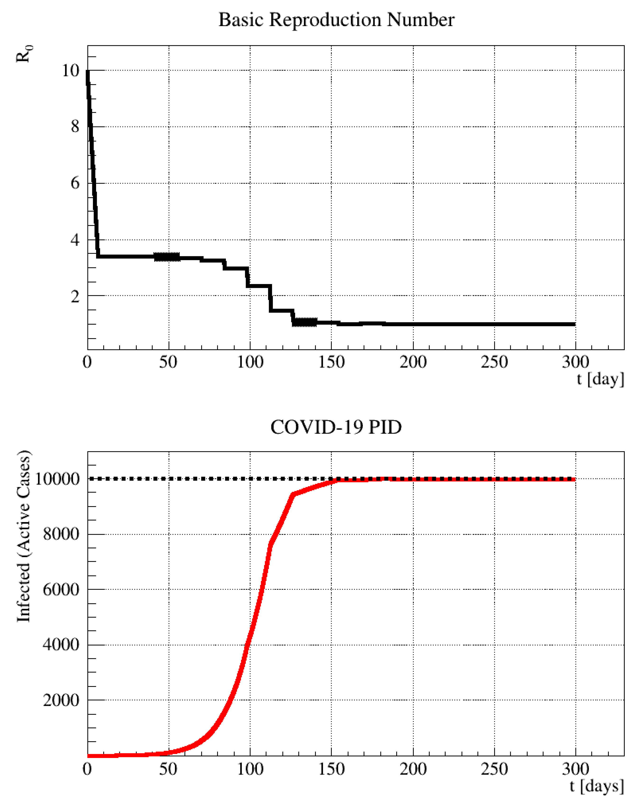
Finally, Figure 6 shows the behaviour of input (top) and output (bottom) with optimal tuning , , and . The optimal tuning, which includes the integral and derivative term, allows reaching the set-point smoothly. This corresponds to a mild lockdown at the beginning and a subsequent fine-tuning of the restriction, corresponding to the final social distancing that can remain unchanged. This scenario is optimal and can be afforded by a country to avoid strong economic damages and finding a good compromise while waiting for a different solution, like vaccination.
Even this last scenario could require further corrections because of many other effects, like the possible change of due to the environmental conditions or to the possible attenuation or increase of the COVID-19 virulence with virus variants. These are the reasons why a warning was made above that the SIR-PID model is only a test-bench theoretical model and that the final fine-tuning can be found probing the real COVID-19 system with PID control actions.
6. Application on Epidemiological Datasets
Working with real data is not trivial due to large fluctuations in the sampled data, essentially due to the intrinsic statistical nature of the phenomenon and, more importantly, due to the discontinuous procedure of the administration of medical tests. For that reason, the computation, especially of the derivative, can be affected by large uncertainty that may cause a false understanding of the system reaction.
It is good practice, therefore, to smooth the data using, for example, a local regression (LOESS) method based on a Savitzky–Golay filter [35]. Once the data are flattened by the smoothing process, the integral can be numerically computed using e.g., Simpson’s rule, while a stable derivative estimation can be performed applying Richardson’s extrapolation method [36].
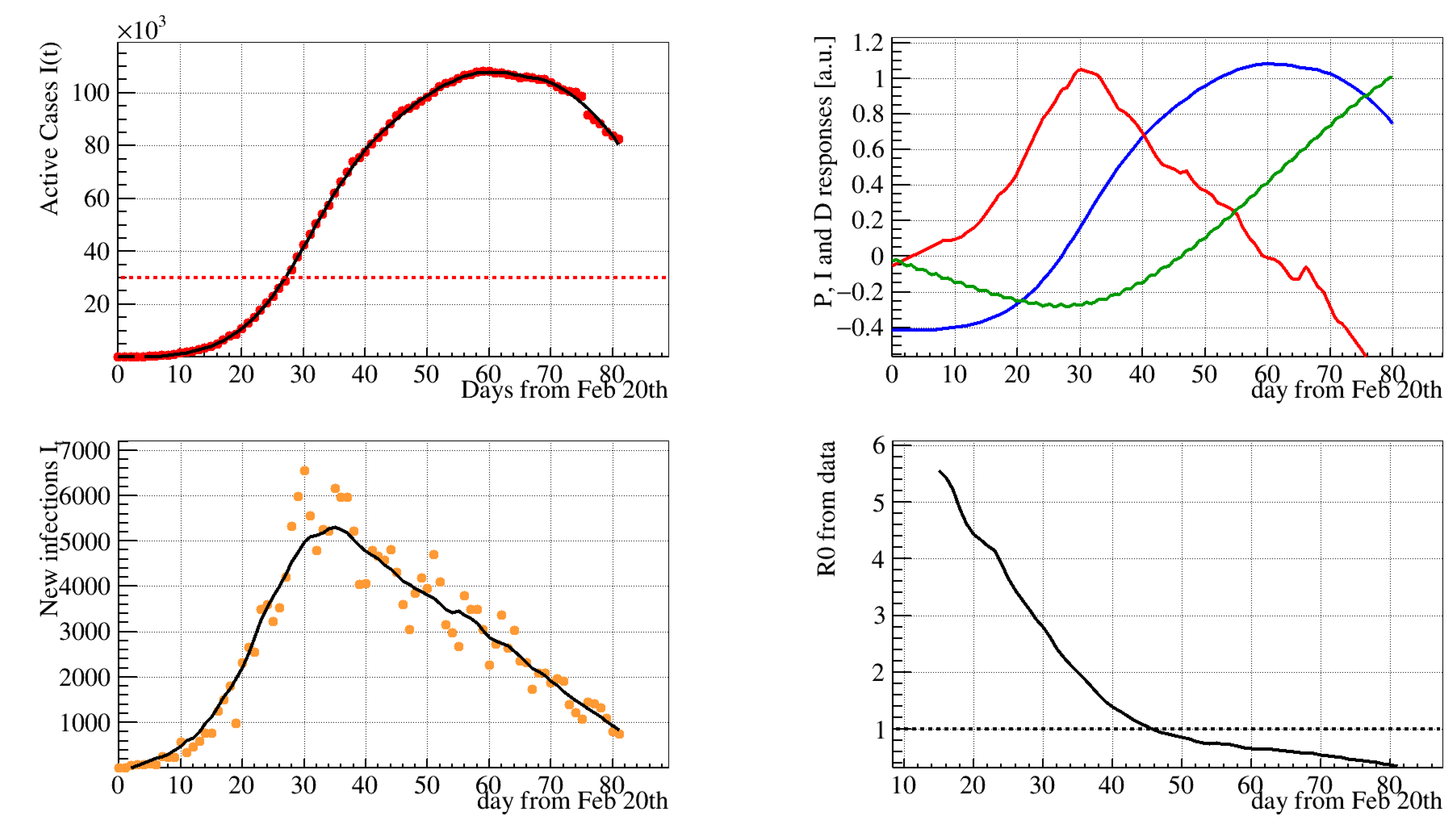
As an example, the analysis of the Italian data during the first epidemic wave in 2020 [17] and its interpretation in terms of the present model are reported. Figure 7 shows the data preparations for the implementation of the PID algorithm on real data. In particular, Figure 7 (top left) shows the active cases evolution, . The black curve represents its smoothing obtained with LOESS. The dashed horizontal line represents a hypothetical set-point of e.g., 30,000 cases for the epidemic control.
Figure 7 (top right), shows the error function, , (blue) of with respect to the chosen set-point and its integral (green) and derivative (red), corresponding to the proportional, the integral and the derivative responses, respectively, as required by the PID method. All of the three functions are built from the smoothed using a LOESS algorithm. Figure 7 (bottom left) reports the daily new infections with its LOESS smoothing (black). Finally, Figure 7 (bottom right) shows the evolution deduced from , using a common method described e.g., in [37]. In particular, the evolving is calculated as
where is the probability of having s days between an infected subject and a new infection caused by the same subject (here assumed to be naively uniform for s in the interval [0, ], e.g., [0, 35] days, see Section 2). is found to decay almost exponentially, as obtained with a different method in [27].
From this particular example, it is clear that the Italian government adopted a slow and progressive restriction policy causing the exponential fall-out. This approach, as shown in Section 4, does not allow the smooth approach to a possible set-point consisting of a few tens of thousands but caused a strong overshoot that required a great deal of time to recover. A different approach would have been considering a correct balance between the P, I, and D terms, as suggested from the PID theory, by looking at the corresponding responses reported in Figure 7 (top right).
In a possible implementation of the PID control method, to be considered as an input parameter even though it is not generally easy to determine this parameter from the data with an ongoing outbreak, see [3]. As a consequence, has to be interpreted, at leading order, in terms of people mobility even if environmental effects and intrinsic changes can modify the COVID-19 virulence. If one makes this simple hypothesis, , from 0 to (10, in the example considered), can be interpreted as 10 levels of people mobility, from drastic lockdown () to free epidemic evolution (). Values in between represent different gradations of the social distancing ruled by official orders set every 14 days, the typical time scale of the COVID-19 epidemic latency. This time could be even shorter, according to the data availability. A day-by-day update of the control is, in principle, possible, however, likely not feasible from a social point of view.
The mobility can be determined a priori considering the daily traffic of different society compartments as, e.g., basic goods production/services, massive industrial production, shops and markets, public transportation, open-air sports, gyms, entertainments, etc. This mobility can include or not the usage of protective devices (as masks, gloves, and disinfectants) and the application of safety distances, or a limited number of indoor people, and so on. Once the mobility scale from 0 to 10 is defined according to mobility/protection estimations, one can test the SIR-PID model on the real COVID-19 data. Probing the system with social restrictions, one can determine the optimal tuning of the SIR-PID coefficient to smoothly reach the desired set-point, thus, minimizing the outbreak damages.
7. Conclusions
In this paper, the use of the proportional–integral–derivative (PID) control theory for the COVID-19 epidemic control is proposed. This well-established technique can be useful both for understanding the behaviour of the infected population during an intermittent lockdown and for defining a strategy for a lockdown policy to establish optimal control. In particular, it is demonstrated that the COVID-19 outbreak, with the attempt at containment through social restrictions by governments, can be modelled and understood in terms of the PID controller mechanism, which is used in various applications of complex systems.
Using a simple time-dependent modification of the SIR modelling of the COVID-19 outbreak evolution, a test-bench model called SIR-PID is built to test the possibility of using a PID controller to achieve the desired containment threshold smoothly, aiming at avoiding serious damages in terms of economical crisis and especially in terms of human life costs. The implementation assumes the basic reproduction number, , as input parameter and the number of infected (or active cases) as output. Even if is not directly accessible as an input parameter, it can be reasonably substituted by people’s mobility, which can be easily estimated and classified in a gradation scale ranging from a drastic lockdown to the free evolution of the pandemic. In addition, a numerical recipe is provided for simulating the epidemic that can be extended to more complex epidemiological models.
In the study, it is shown that, in using a loop-tuning procedure, this goal was achievable in a satisfactory way. This result allows us to exploit this procedure on real data, even if the real COVID-19 outbreak system is more complex due to other potential effects contributing to the time variation of . For the basic model considered, it is shown that the best way of achieving an optimal control is to react promptly at the beginning of the pandemic by lowering the mobility by a factor of two and then to increase the social restrictions slowly to reach the desired set-point that is deemed affordable for the healthcare system. This procedure is desirable when the pandemic is already out of control over a wide geographical area because the first attempt should be the complete confinement of the outbreak by drastically limiting the patient zero areas and nearest contacts, when possible.
The advantage of using a well-known PID control theory instead of relying on traditional control methods, based on numerical simulations and rules suggested by the experience, is mainly its flexibility. Once the input and output variables have been selected, the PID controller, through the tuning process, can probe the system and calibrate the parameters—the proportional, integral and derivative terms — even the features of the system are not perfectly known and cannot be simulated a priori.
Furthermore, instead of delaying the epidemic peaks and relaxations (waves), this allows us to smoothly approach the desired set-point (in principle, changeable during the different phases of the pandemic) and to keep it almost constant, in compliance with the healthcare system availability. If the epidemic model can be simulated, the tuning process is even faster, as, in this case, the PID parameter, as in the SIR example, can be determined from the theory. A good epidemic modelling, even if not perfectly correct, is useful for sketching out the preliminary configuration and is further improvable on real data with subsequent fine-tuning.
In this study, the case of keeping the number of infectious people, close to the threshold set-point is mainly discussed, approaching it smoothly and avoiding strong overshoots. However, when the conditions for the propagation of the virus drastically change (e.g., due to a vaccination campaign) the conditions naturally changes to . In other words, the system, even if completely released, would not be able to increase any further. At this moment, an “exit strategy” is needed. There are two options: (i) maintaining the PID coefficients as they are and waiting for the epidemic to extinguish naturally; or (ii) further reducing, when possible, the set-point, thus, decreasing the mobility to speed up the conclusion of the epidemic and eventually the return to normality.
In addition to the simple SIR model, the SIR-PID is proposed here as a starting point for an interdisciplinary approach in epidemiology. More complex models can be elaborated without changing the core of the problem: the epidemic control is an input–output system that is sufficiently complex and needs to be stabilized around a desired set-point, and this is a problem that is very well approached and solved in PID controller theory.
Author Contributions
Conceptualization, A.I. and N.R.; methodology, A.I. and N.R.; software, A.I. and N.R.; validation, A.I. and N.R.; formal analysis, A.I. and N.R.; writing—original draft preparation, A.I. and N.R.; writing—review and editing, A.I. and N.R. All authors have read and agreed to the published version of the manuscript.
Funding
This research received no external funding.
Institutional Review Board Statement
Not applicable.
Informed Consent Statement
Not applicable.
Data Availability Statement
The paper does not present other data but the ones explicitly mentioned in the paper. Every plot is basically reproducible using the information contained in the text.
Acknowledgments
We would like to thank also Francesca Baldinelli for helping in understating some details about and Guido Baldinelli for explanations about the medical meaning of different COVID-19 aspects. We also thank all people contributing to proofreading.
Conflicts of Interest
The authors declare no conflict of interest.
References
- World Health Organization (WHO): Coronavirus. Available online: https://www.who.int/health-topics/coronavirus/ (accessed on 25 June 2021).
- Hu, B.; Guo, H.; Zhou, P.; Shi, Z.L. Characteristics of SARS-CoV-2 and COVID-19. Nat. Rev. Microbiol. 2021, 19, 141–154. [Google Scholar] [CrossRef] [PubMed]
- Delamater, P.L.; Street, E.J.; Leslie, T.F.; Yang, Y.; Jacobsen, K.H. Complexity of the basic reproduction number (R0). Emerg. Infect. Dis. 2019, 25, 1–4. [Google Scholar] [CrossRef] [Green Version]
- Preliminary Estimate of Excess Mortality During the COVID-19 Outbreak—New York City, 11 March–1 May 2020. Morb. Mortal Wkly. Rep. (MMWR) 2020, 69, 603–605. [CrossRef]
- Anderson, R.M.; Heesterbeek, H.; Klinkenberg, D.; Hollingsworth, T.D. Déirdre Hollingsworth. How will country-based mitigation measures influence the course of the COVID-19 epidemic? Lancet 2020, 395, 931–934. [Google Scholar] [CrossRef]
- Bontempi, E.; Vergalli, S.; Squazzoni, F. Understanding Covid-19 diffusion requires an interdisciplinary, multi-dimensional approach. Environ. Res. 2020, 188, 109814. [Google Scholar] [CrossRef] [PubMed]
- Bertozzi, A.L.; Franco, E.; Mohler, G.; Short, M.B.; Sledge, D. The challenges of modeling and forecasting the spread of COVID-19. Proc. Natl. Acad. Sci. USA 2020, 117, 16732–16738. [Google Scholar] [CrossRef] [PubMed]
- Ledzewicz, U.; Schättle, H. On optimal singular controls for a general SIR-model with vaccination and treatment. Am. Inst. Math. Sci. Conf. Publ. 2011, 2011, 981–990. [Google Scholar]
- Alvarez, F.E.; Argente, D.; Lippi, F. A Simple Planning Problem for COVID-19 Lockdown; NBER Working Papers 26981; National Bureau of Economic Research: Cambridge, MA, USA, 2020. [Google Scholar] [CrossRef]
- Milani, F. COVID-19 outbreak, social response, and early economic effects: A Global VAR analysis of cross-country interdependencies. J. Popul. Econ. 2021, 34, 223–252. [Google Scholar] [CrossRef] [PubMed]
- WHO: Evaluation of COVID-19 Vaccine Effectiveness. Available online: https://www.who.int/publications/i/item/WHO-2019-nCoV-vaccine_effectiveness-measurement-2021.1 (accessed on 25 June 2021).
- WHO: Q&As on COVID-19 and Related Health Topics. Available online: https://www.who.int/emergencies/diseases/novel-coronavirus-2019/question-and-answers-hub (accessed on 25 June 2021).
- Feoli, A.; Iannella, A.L.; Benedetto, E. Spreading of COVID-19 in Italy as the spreading of a wave packet. Eur. Phys. J. Plus 2020, 135, 644. [Google Scholar] [CrossRef]
- Olney, A.M.; Smith, J.; Sen, S.; Thomas, F.; Unwin, H.J.T. Estimating the effect of social distancing interventions on COVID-19 in the United States. Am. J. Epidemiol. 2021, kwaa293. [Google Scholar] [CrossRef]
- Padhi, A.; Pradhan, S.; Sahoo, P.P.; Suresh, K.; Behera, B.K.; Panigrahi, P.K. Studying the effect of lockdown using epidemiological modelling of COVID-19 and a quantum computational approach using the Ising spin interaction. Sci. Rep. 2020, 10, 21741. [Google Scholar] [CrossRef]
- Yung, C.; Saffari, E.; Liew, C. Time to Rt < for COVID-19 public health lockdown measures. Epidemiol. Infect. 2020, 148, E301. [Google Scholar] [PubMed]
- Available online: https://www.worldometers.info/coronavirus/ (accessed on 25 June 2021).
- Stuart, B. A History of Control Engineering 1930–1955; Peter Peregrinus Ltd./IEE: London, UK, 1993; p. 48. Available online: https://www.scribd.com/document/490573330/A-History-of-Control-Engineering-1930-1955-Bennett-pdf (accessed on 25 June 2021).
- Borase, R.P.; Maghade, D.K.; Sondkar, S.Y.; Pawar, S.N. A review of PID control, tuning methods and applications. Int. J. Dyn. Control 2021, 9, 818–827. [Google Scholar] [CrossRef]
- Nicolas, M. Directional stability of automatically steered bodies. J. Am. Soc. Naval Eng. 1922, 34, 280–309. [Google Scholar] [CrossRef]
- Francis, M. A biomolecular proportional integral controller based on feedback regulations of protein level and activity. R. Soc. Open Sci. 2018, 5, 171966. [Google Scholar]
- Chevalier, M.; Gómez-Schiavon, M.; Ng, A.H.; El-Samad, H. Design and analysis of a proportional–integral–derivative controller with biological molecules. Cell Syst. 2019, 9, 338–353. [Google Scholar] [CrossRef] [PubMed]
- Bansal, H.; Sharma, R.; Ponpathirkoottam, S. PID controller tuning techniques: A review. J. Control Eng. Technol. 2012, 2, 168–176. Available online: https://www.academia.edu/11729116/PID_Controller_Tuning_Techniques_A_Review (accessed on 25 June 2021).
- George, T.; Ganesan, V. Optimal tuning of PID controller in time delay system: A review on various optimization techniques. Chem. Prod. Process. Model. 2021, in press. [Google Scholar]
- Kermack, W.O.; McKendrick, A.G. A contribution to the mathematical theory of epidemics. Proc. R. Soc. Lond. A: Math. Phys. Eng. Sci. 1927, 115, 700–721. [Google Scholar]
- Cooper, I.; Mondal, A.; Antonopoulos, C.G. A SIR model assumption for the spread of COVID-19 in different communities. Chaos Solitons Fractals 2020, 139, 110057. [Google Scholar] [CrossRef] [PubMed]
- Ianni, A.; Rossi, N. Describing the COVID-19 outbreak during the lockdown: Fitting modified SIR models to data. Eur. Phys. J. Plus 2020, 135, 885. [Google Scholar] [CrossRef] [PubMed]
- Giordano, G.; Blanchini, F.; Bruno, R.; Colaneri, P.; Di Filippo, A.; Di Matteo, A.; Colaneri, M. Modelling the COVID-19 epidemic and implementation of population-wideinterventions in Italy. Nat. Med. 2020, 26, 855–860. [Google Scholar] [CrossRef] [PubMed]
- Langfeld, K. Dynamics of epidemic diseases without guaranteed immunity. J. Math. Ind. 2021, 11, 5. [Google Scholar] [CrossRef] [PubMed]
- Runge, C. Ueber die numerische Auflösung von Differentialgleichungen. Math. Ann. 1895, 46, 167–178, Original paper. [Google Scholar] [CrossRef] [Green Version]
- Kutta, W. Beitrag zur näherungsweisen Integration totaler Differentialgleichungen. Z. Math. Phys. 1901, 46, 435–453, Original paper. [Google Scholar]
- Euler, L. Institutionum Calculi Integralis; Original; PETROPOLI Impenfis Academiae Imperialis Scientiarum: St. Petersburg, Russian Empire, 1768; Volumes I–III, Available online: https://archive.org/details/institutionescal020326mbp/page/n33/mode/2up (accessed on 25 June 2021).
- Ziegler, J.G.; Nichols, N.B. Optimum settings for automatic controllers. J. Dyn. Syst. Meas. Control 1993, 115, 220–222. [Google Scholar] [CrossRef]
- Ang, K.H.; Chong, G.; Li, Y. PID control system analysis, design, and technology. IEEE Trans. Control Syst. Technol. 2005, 13, 559–576. [Google Scholar] [CrossRef] [Green Version]
- Savitzky, A.; Golay, M.J.E. Smoothing and differentiation of data by simplified least squares procedures. Anal. Chem. 1964, 36, 1627–1639. [Google Scholar] [CrossRef]
- Richardson, L.F. The approximate arithmetical solution by finite differences of physical problems including differential equations, with an application to the stresses in a masonry dam. Philos. Trans. R. Soc. A: Math. Phys. Eng. Sci. 1911, 210, 459–470. [Google Scholar] [CrossRef] [Green Version]
- Cori, A.; Cauchemez, S.; Ferguson, N.M.; Fraser, C.; Dahlqwist, E.; Demarsh, P.A.; Jombart, T.; Kamvar, Z.N.; Lessler, J.; Li, S.; et al. EpiEstim: Estimate Time Varying Reproduction Numbers from Epidemic Curves. Available online: https://cran.r-project.org/package=EpiEstim (accessed on 25 June 2021).
Figure 1.
Flow diagram of the proportional–integral–derivative controller (PID) controller. The time t-dependent error function, , is the difference between the set-point (SP) and a measured process variable (PV). The weighted average of the P, I, and D contributions determines the output control, , for the specific system to be controlled.

Figure 2.
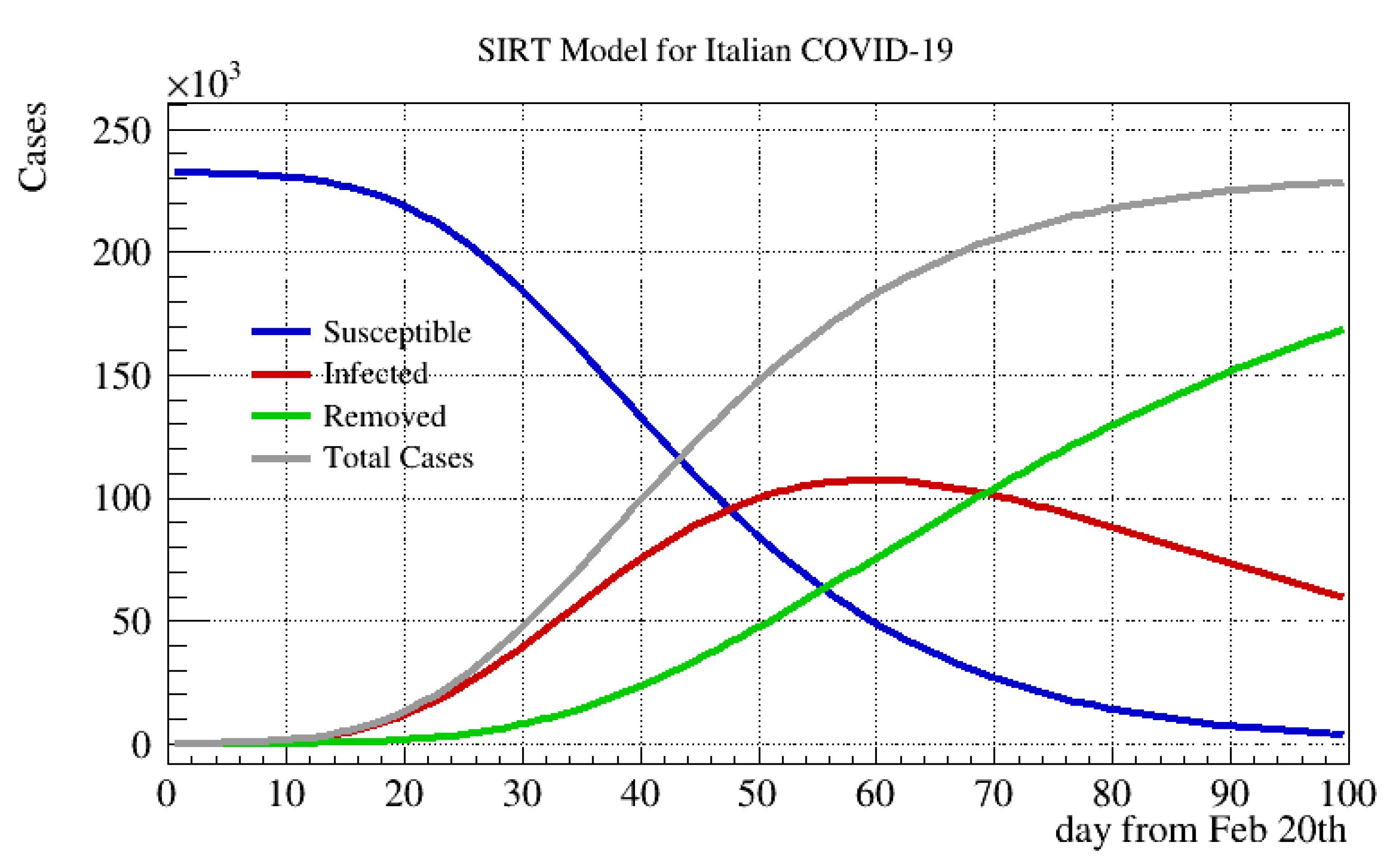
Example of time-dependent susceptible–infectious–recovered (SIR) model prediction, in which the basic reproduction number decreases exponentially from the beginning of the disease epidemic outbreak. The initial susceptible population S (blue) is converted into infected I (red) according to the time-dependent basic reproduction number, . Finally, according to the strength of the recovery rate,, population I is converted into removed R (green). The grey curve represents the sum of R+I, and is usually very well approximated by a logistic curve (the parameters used in these examples are days, where is the transition rate, and days).
Figure 2.
Example of time-dependent susceptible–infectious–recovered (SIR) model prediction, in which the basic reproduction number decreases exponentially from the beginning of the disease epidemic outbreak. The initial susceptible population S (blue) is converted into infected I (red) according to the time-dependent basic reproduction number, . Finally, according to the strength of the recovery rate,, population I is converted into removed R (green). The grey curve represents the sum of R+I, and is usually very well approximated by a logistic curve (the parameters used in these examples are days, where is the transition rate, and days).

Figure 3.
Tuning example: simulation of a generic system responding respectively to a pure proportional control (red), a proportional corrected with the integral term (yellow) for removing the bias with the set-point (dashed black) and finally with oscillation damped by the integral term (violet). The values used here for the proportinal, derivative, and integral terms are , , and , respectively.

Figure 4.
Example of PID controller simulation. Behaviour of (top) the input basic reproduction number, , and (bottom) the output number of the infectious individuals, , with , . The dashed black line represents the set-point. A very strong proportional action only is not able to stabilize the system. This corresponds to the complete absence of restrictions at the beginning and a drastic lockdown when the threshold is reached, and this behaviour is repeated every time the set-point is reached, causing many out-of-control devastating epidemic waves.

Figure 5.
Example of PID controller simulation. Behaviour of (top) the input basic reproduction number, , and (bottom) the output number of the infectious individuals, , with and . The dashed black line represents the set-point. A mild proportional term avoids a strong overshoot at the first reach of the set-point but is not sufficient for damping the system oscillation. This corresponds to a less drastic social restriction at the beginning and then a subsequent attempt to stabilize the rate with the mild and strong lockdowns.

Figure 6.
Example of PID controller simulation. Behaviour of (top) input basic reproduction number, , and (bottom) the output number of the infectious individuals, , with tuned , , and . The dashed black line represents the set-point. The optimal tuning, which includes the integral and derivative term, allows reaching the set-point smoothly. This corresponds to a mild lockdown at the beginning and a subsequent fine tuning of the restriction corresponding to the final social distancing that can remain unchanged.

Figure 7.
Top left: Active cases in Italy during the first epidemic wave in 2020. The black curve represents its smoothing obtained with the local regression method (LOESS). The dashed horizontal line represents a hypothetical set-point of, e.g., 30,000 cases. Top right: (in arbitrary units) The error function (blue) of with respect to the chosen set-point and its integral (green) and derivative (red), corresponding to the proportional, the integral, and the derivative responses, respectively, as required by the PID method. All of the three functions are built from the smoothed . Bottom left: Daily new infections, , with its LOESS smoothing (black). Bottom right: evolution deduced from ; see text for details.

Publisher’s Note: MDPI stays neutral with regard to jurisdictional claims in published maps and institutional affiliations. |
© 2021 by the authors. Licensee MDPI, Basel, Switzerland. This article is an open access article distributed under the terms and conditions of the Creative Commons Attribution (CC BY) license (https://creativecommons.org/licenses/by/4.0/).
Share and Cite
MDPI and ACS Style
Ianni, A.; Rossi, N. SIR-PID: A Proportional–Integral–Derivative Controller for COVID-19 Outbreak Containment. Physics 2021, 3, 459-472. https://0-doi-org.brum.beds.ac.uk/10.3390/physics3030031
AMA Style
Ianni A, Rossi N. SIR-PID: A Proportional–Integral–Derivative Controller for COVID-19 Outbreak Containment. Physics. 2021; 3(3):459-472. https://0-doi-org.brum.beds.ac.uk/10.3390/physics3030031
Chicago/Turabian StyleIanni, Aldo, and Nicola Rossi. 2021. "SIR-PID: A Proportional–Integral–Derivative Controller for COVID-19 Outbreak Containment" Physics 3, no. 3: 459-472. https://0-doi-org.brum.beds.ac.uk/10.3390/physics3030031