Spatially Developing Modes: The Darcy–Bénard Problem Revisited

Abstract

In this paper, the instability resulting from small perturbations of the Darcy–Bénard system is explored. An analysis based on time–periodic and spatially developing Fourier modes is adopted. The system under examination is a horizontal porous layer saturated by a fluid. The two impermeable and isothermal plane boundaries are considered to have different temperatures, so that the porous layer is heated from below. The spatial instability for the system is defined by taking into account both the spatial growth rate of the perturbation modes and their propagation direction. A comparison with the neutral stability condition determined by using the classical spatially periodic and time–evolving Fourier modes is performed. Finally, the physical meaning of the concept of spatial instability is discussed. In contrast to the classical analysis, based on spatially periodic modes, the spatial instability analysis, involving time–periodic Fourier modes, is found to lead to the conclusion that instability occurs whenever the Rayleigh number is positive.

1. Introduction

Under the current terminology, the Darcy–Bénard problem designates the study of the onset of convection in a horizontal porous layer saturated by a fluid and bounded by parallel plane walls at different temperatures. As the lower boundary temperature is the largest, the mechanism for the onset of convection cells in the porous layer is the buoyancy force caused by heating from below. The alternative name for this topic is the Horton–Rogers–Lapwood problem. The denomination Darcy–Bénard focusses on the application of Darcy’s law as a model of flow in a porous medium and to the Rayleigh–Bénard nature of the instability as induced by the thermal buoyancy force [1,2]. On the other hand, by referring to this problem as Horton–Rogers–Lapwood, one recognises the pioneering contributions by Horton and Rogers [3] and by Lapwood [4] for its formulation and solution. The considerably broad literature regarding the Darcy–Bénard problem has been reviewed by several authors [5,6,7,8,9].

The usual approach to the solution of the Darcy–Bénard problem is the linear stability analysis. This analysis is usually carried out by testing how spatially periodic and time–evolving Fourier modes of perturbation affect the basic conduction state. In this state, the fluid is motionless and a uniform downward temperature gradient yields a potentially unstable thermal stratification of the fluid [5,8]. A different method for the linear stability analysis of stationary shear flows is based on a different class of perturbation modes, namely time–periodic and spatially–developing Fourier modes [2,10,11,12]. In particular, Chapter 7 of Schmid and Henningson [12] provides a detailed analysis of the spatially–developing perturbations, exemplified for the Poiseuille flow.

The aim of this paper is a revisitation of the Darcy–Bénard problem from the perspective of spatial stability analysis. The latter is a shorthand for the method based on the spatially–developing Fourier modes of perturbation having a periodic dependence on time. The physical difference between the traditional stability analysis, based on spatially–periodic modes, and the spatial stability analysis, based on time–periodic modes, is described in detail. The predictions of the spatial stability analysis for the Darcy–Bénard problem are presented and discussed showing that Fourier modes exponentially–growing in space along their direction of propagation exist for every positive value of the Rayleigh number.

2. Mathematical Model

The objective of the present paper is the study of a fluid–saturated porous layer with a thickness H and an infinite horizontal width. The z axis is considered to be oriented vertically so that the gravitational acceleration is given by $\mathbf{g}=-g{\mathbf{e}}_z$, where g is the modulus of g, and ${\mathbf{e}}_z$ is the unit vector in the z direction. The horizontal planes $z=0$ and $z=H$ are kept at uniform temperatures $T_h$ and $T_c$, respectively. Here, subscripts h and c are meant to denote hot and cold boundaries, which is the typical setup for the Darcy–Bénard problem. The x and y axes are horizontal. The seepage flow in the porous medium is modelled through Darcy’s law. The Oberbeck–Boussinesq approximation is employed as a model of the thermal buoyancy force acting on the fluid [8].

2.1. Non–Dimensional Analysis

Let us introduce scaled quantities in order to express the governing equations in a non–dimensional form:

$$\begin{array}{c}(x^{*},y^{*},z^{*})=\frac{(x,y,z)}{H}, t^{*}=\frac{t}{\sigma H^2/\alpha }, {\mathbf{u}}^{*}=\frac{\mathbf{u}}{\alpha /H}\\ p^{*}=\frac{p}{\mu \alpha /K}, T^{*}=\frac{T-T_c}{T_h-T_c}.\end{array}$$

(1)

Furthermore, the Rayleigh number is defined as

$$\begin{array}{c}\begin{array}{c}\hfill R=\frac{g\beta (T_h-T_c)KH}{\nu \alpha }.\end{array}\end{array}$$

(2)

In Equations (1) and (2), t is the time, u is the seepage velocity with Cartesian components $(u,v,w)$, p is the local difference between the pressure and the hydrostatic pressure, and T is the temperature. The symbols $\alpha$, $\mu$, $\nu$, $\beta$, K and $\sigma$ stand for the average thermal diffusivity of the saturated porous medium, the dynamic viscosity of the fluid, the kinematic viscosity of the fluid, the thermal expansion coefficient of the fluid, the permeability of the porous medium and the heat capacity ratio, respectively. In fact, the quantity $\sigma$ is the ratio between the average volumetric heat capacity of the porous medium and that of the saturating fluid. The starred quantities defined by Equation (1) are non–dimensional. Since the forthcoming analysis will be entirely formulated in non–dimensional terms, the stars will be hereafter omitted for the sake of brevity. The notation $(T_h,T_c)$ for the dimensional boundary temperatures tacitly presumes that $T_h>T_c$, which is the usual situation of heating–from–below and unstable thermal stratification characteristic of the Rayleigh–Bénard system. This entails $R>0$, whereas a negative Rayleigh number signifies the opposite situation of heating–from–above.

The non–dimensional form of the local mass, momentum and energy balance equations is given by [8]:

$$\begin{array}{c}\mathbf{\nabla }\mathbf{·}\mathbf{u}=0,\end{array}$$

(3a)

$$\begin{array}{c}\mathbf{u}=-\mathbf{\nabla }p+RT{\mathbf{e}}_z,\end{array}$$

(3b)

$$\begin{array}{c}\frac{\partial T}{\partial t}+\mathbf{u}\mathbf{·}\mathbf{\nabla }T={\nabla }^{2}T.\end{array}$$

(3c)

Such governing equations are subject to the boundary conditions:

$$\begin{array}{c}\begin{array}{c}\hfill w(x,y,0,t)=0=w(x,y,1,t), T(x,y,0,t)=1, T(x,y,1,t)=0,\end{array}\end{array}$$

(4)

which express the impermeability of the boundaries and their uniform dimensionless temperatures, 1 and 0.

2.2. Basic Conduction State and Perturbations

A steady state of the system exists where the heat transfer across the porous layer is one of pure conduction. A time–independent solution of Equations (3) and (4) for this state, denoted with the subscript 0, is given by

$$\begin{array}{c}\begin{array}{c}\hfill {\mathbf{u}}_0=0, T_0=1-z, \mathbf{\nabla }{p}_0=R(1-z){\mathbf{e}}_z.\end{array}\end{array}$$

(5)

In order to test the stability of such a steady state, the standard procedure is perturbing the system. Here, one assumes linear or small–amplitude perturbations $(\mathbf{U},P,\Theta )$ such that:

$$\begin{array}{c}\begin{array}{c}\hfill \mathbf{u}={\mathbf{u}}_0+\epsilon \mathbf{U}, p=p_0+\epsilon P, T=T_0+\epsilon \Theta ,\end{array}\end{array}$$

(6)

where $\epsilon$ is a small perturbation parameter, i.e., $\left|\epsilon \right|\ll 1$. Let us now substitute Equations (5) and (6) into Equations (3) and (4) and simplify terms $\mathcal{O}\left({\epsilon }^2\right)$:

$$\begin{array}{c}\mathbf{\nabla }\mathbf{·}\mathbf{U}=0,\end{array}$$

(7a)

$$\begin{array}{c}\mathbf{U}=-\mathbf{\nabla }P+R\Theta {\mathbf{e}}_z,\end{array}$$

(7b)

$$\begin{array}{c}\frac{\partial \Theta }{\partial t}-W={\nabla }^2\Theta ,\end{array}$$

(7c)

$$\begin{array}{c}W(x,y,0,t)=0=W(x,y,1,t), \Theta (x,y,0,t)=0=\Theta (x,y,1,t),\end{array}$$

(7d)

where $(U,V,W)$ represent the Cartesian components of U. In Equations (7), $\epsilon$–dependence is simplified due to the linearisation.

One can recognize that Equations (7) are invariant with respect to rotations around the z axis, so that any horizontal direction is just equivalent. Then, the analysis can be made two–dimensional by assuming independence from the coordinate y, so that the perturbation fields are defined in the $xz$ plane and V is zero. With this understanding, one can introduce a perturbation stream function defined as

$$\begin{array}{c}\begin{array}{c}\hfill U=\frac{\partial \Psi }{\partial z}, W=-\frac{\partial \Psi }{\partial x}.\end{array}\end{array}$$

(8)

Thus, Equations (7) can be rewritten as

$$\begin{array}{c}{\nabla }^2\Psi =-R\frac{\partial \Theta }{\partial x},\end{array}$$

(9a)

$$\begin{array}{c}{\nabla }^2\Theta =\frac{\partial \Theta }{\partial t}+\frac{\partial \Psi }{\partial x},\end{array}$$

(9b)

$$\begin{array}{c}\Psi (x,0,t)=0=\Psi (x,1,t), \Theta (x,0,t)=0=\Theta (x,1,t).\end{array}$$

(9c)

The solution of Equations (9) may be expressed through Fourier sine series in the z coordinate, so that Equation (9c) is identically satisfied. In fact, let us introduce the notation,

$$\begin{array}{c}\begin{array}{c}\hfill \mathbb{F}=\left(\begin{array}{c}\Psi \\ \Theta \end{array}\right),\end{array}\end{array}$$

(10)

where $\mathbb{F}(x,z,t)$ can be considered as a perturbation (two–dimensional) vector function. A straightforward way to express the dependence on z is by employing sine Fourier series, so that:

$$\begin{array}{c}\begin{array}{c}\hfill \mathbb{F}(x,z,t)=\sum _{n=1}^{\infty }{\mathbb{F}}_n(x,t)sin\left(n\pi z\right).\end{array}\end{array}$$

(11)

Equations (9) now read:

$$\begin{array}{c}\frac{{\partial }^2{\Psi }_n}{\partial x^2}-{\left(n\pi \right)}^2{\Psi }_n=-R\frac{\partial {\Theta }_n}{\partial x},\end{array}$$

(12a)

$$\begin{array}{c}\frac{{\partial }^2{\Theta }_n}{\partial x^2}-{\left(n\pi \right)}^2{\Theta }_n=\frac{\partial {\Theta }_n}{\partial t}+\frac{\partial {\Psi }_n}{\partial x},\end{array}$$

(12b)

for every $n=1,2,$ etc.

In Section 3 and Section 4, two different paths are considered to complete the solution of the Darcy–Bénard problem. The one discussed in Section 3 is simple and widely known in the literature [5,6,7,8,9]. On the other hand, the procedure, discussed in Section 4, is more complicated, while disclosing new elements of appraisement and new insights into the Darcy–Bénard problem.

3. Spatially Periodic Fourier Modes

The Fourier transform of ${\mathbb{F}}_n(x,t)$ can be defined as [13]:

$$\begin{array}{c}\begin{array}{c}\hfill {\widehat{\mathbb{F}}}_n(k,t)=\frac{1}{\sqrt{2\pi }}\underset{-\infty }{\overset{+\infty }{\int }}{\mathbb{F}}_n(x,t)e^{-ikx}\mathrm{d}x,\end{array}\end{array}$$

(13)

with its inverse transform given by

$$\begin{array}{c}\begin{array}{c}\hfill {\mathbb{F}}_n(x,t)=\frac{1}{\sqrt{2\pi }}\underset{-\infty }{\overset{+\infty }{\int }}{\widehat{\mathbb{F}}}_n(k,t)e^{ikx}\mathrm{d}k.\end{array}\end{array}$$

(14)

The transformation variable is the coordinate x, so that k is endowed with the physical meaning of a wave number. Equation (14) evidences that the perturbation vector $\mathbb{F}$ is expressed as the linear combination of spatially–periodic wavelike signals, each one with a periodicity along the x axis given by $2\pi /k$.

The Fourier transform, when applied to Equations (12), yields:

$$\begin{array}{c}[{\left(n\pi \right)}^2+k^2]{\widehat{\Psi }}_n-ikR{\widehat{\Theta }}_n=0,\end{array}$$

(15a)

$$\begin{array}{c}[{\left(n\pi \right)}^2+k^2]{\widehat{\Theta }}_n+\frac{\partial {\widehat{\Theta }}_n}{\partial t}+ik{\widehat{\Psi }}_n=0.\end{array}$$

(15b)

The solution of Equations (15) is:

$$\begin{array}{c}\begin{array}{c}\hfill {\widehat{\Psi }}_n(k,t)=\frac{ikR}{{\left(n\pi \right)}^2+k^2}{\widehat{\Theta }}_n(k,0)e^{\lambda t}, {\widehat{\Theta }}_n(k,t)={\widehat{\Theta }}_n(k,0)e^{\lambda t},\end{array}\end{array}$$

(16)

with:

$$\begin{array}{c}\begin{array}{c}\hfill \lambda =-[{\left(n\pi \right)}^2+k^2]+\frac{k^{2}R}{{\left(n\pi \right)}^2+k^2}.\end{array}\end{array}$$

(17)

Equations (16) and (17) allow us to finalise the linear stability analysis. The perturbation modes ${\widehat{\Psi }}_n$ and ${\widehat{\Theta }}_n$ grow exponentially in time when, for a given wave number k, R exceeds the threshold ${[{\left(n\pi \right)}^2+k^2]}^2/k^2$, while they are damped exponentially in time if R is smaller than this threshold. The former condition delineates the instability of the Darcy–Bénard system, while the latter identifies the stability. Therefore, the marginal condition between stability and instability is:

$$\begin{array}{c}\begin{array}{c}\hfill R=\frac{{[{\left(n\pi \right)}^2+k^2]}^2}{k^2}.\end{array}\end{array}$$

(18)

The minimum value of R along the marginal stability curve is the critical value, $R_{\mathrm{c}}$. It is achieved with $n=1$ and is given by $R_{\mathrm{c}}=4{\pi }^2$, which corresponds to the critical wave number $k_{\mathrm{c}}=\pi$ [8].

4. Time–Periodic Fourier Modes

Let us now explore an alternative approach to the Fourier transform solution described in Section 3. Let us define the Fourier transform of ${\mathbb{F}}_n(x,t)$ as:

$$\begin{array}{c}\begin{array}{c}\hfill {\tilde{\mathbb{F}}}_n(x,\omega )=\frac{1}{\sqrt{2\pi }}\underset{-\infty }{\overset{+\infty }{\int }}{\mathbb{F}}_n(x,t)e^{i\omega t}\mathrm{d}t,\end{array}\end{array}$$

(19)

so that the inverse transform is given by:

$$\begin{array}{c}\begin{array}{c}\hfill {\mathbb{F}}_n(x,t)=\frac{1}{\sqrt{2\pi }}\underset{-\infty }{\overset{+\infty }{\int }}{\tilde{\mathbb{F}}}_n(x,\omega )e^{-i\omega t}\mathrm{d}\omega .\end{array}\end{array}$$

(20)

In Equations (19) and (20), the transformation variable is the time t, and $\omega$ represents the angular frequency. Equation (20) implies that the perturbation vector $\mathbb{F}$ is a linear combination of time–periodic wavelike signals, each one with a periodicity in time given by $2\pi /\omega$. By applying the Fourier transform (19) to Equations (12), one finds:

$$\begin{array}{c}\frac{{\partial }^2{\tilde{\Psi }}_n}{\partial x^2}-{\left(n\pi \right)}^2{\tilde{\Psi }}_n=-R\frac{\partial {\tilde{\Theta }}_n}{\partial x},\end{array}$$

(21a)

$$\begin{array}{c}\frac{{\partial }^2{\tilde{\Theta }}_n}{\partial x^2}-{\left(n\pi \right)}^2{\tilde{\Theta }}_n=-i\omega {\tilde{\Theta }}_n+\frac{\partial {\tilde{\Psi }}_n}{\partial x}.\end{array}$$

(21b)

Much like as in Section 3, the solution of Equations (21) can be expressed as:

$$\begin{array}{c}{\tilde{\Psi }}_n(x,\omega )={\tilde{\Theta }}_n(0,\omega )\sum _{j=1}^4\frac{C_j{\eta }_{j}R}{{\left(n\pi \right)}^2-{\eta }_j^2}{e}^{{\eta }_{j}x},\\ {\tilde{\Theta }}_n(x,\omega )={\tilde{\Theta }}_n(0,\omega )\sum _{j=1}^4{C}_j{e}^{\eta x},\end{array}$$

(22)

where $C_1,C_2,C_3$ and $C_4$ are coefficients such that ${\sum }_{j=1}^4{C}_j=1$ and ${\eta }_1,{\eta }_2,{\eta }_3$ and ${\eta }_4$ are the four roots of the equation,

$$\begin{array}{c}\begin{array}{c}\hfill [{\left(n\pi \right)}^2-{\eta }^2][{\left(n\pi \right)}^2-{\eta }^2-i\omega ]+{\eta }^{2}R=0.\end{array}\end{array}$$

(23)

The complication emerging from Equations (22) and (23) is two–fold. First, the exponential parameter $\eta$ is complex, while $\lambda$ in Equation (17) is real. Second, $\eta$ is defined only implicitly through Equation (23), whereas $\lambda$ is explicitly expressed by Equation (17). The real and imaginary parts of $\eta$ can be denoted as

$$\begin{array}{c}\begin{array}{c}\hfill \eta =s+ik,\end{array}\end{array}$$

(24)

where s represents the exponential growth rate in the x direction, while k is the wave number. For every given pair $(R,n)$, one obtains four different branches $\eta \left(\omega \right)$ by solving the algebraic Equation (23).

One can rescale the variables $\eta$, $\omega$ and R, so that:

$$\begin{array}{c}\begin{array}{c}\hfill {\eta }^{\prime }=\frac{\eta }{n}, {\omega }^{\prime }=\frac{\omega }{n^2}, R^{\prime }=\frac{R}{n^2}.\end{array}\end{array}$$

(25)

With the scaled variables, Equation (23) is rewritten as:

$$\begin{array}{c}\begin{array}{c}\hfill ({\pi }^2-{\eta }^{{}^{\prime }2})({\pi }^2-{\eta }^{{}^{\prime }2}-i{\omega }^{\prime })+{\eta }^{{}^{\prime }2}{R}^{\prime }=0,\end{array}\end{array}$$

(26)

which is, in fact, the $n=1$ version of Equation (23). Hereafter, the primes in the scaled symbols, defined by Equation (25), are omitted. This is definitely equivalent to assuming $n=1$ in Equation (23). In what follows, one must keep in mind that any predicted value of, say, $\eta$ has to be multiplied by n whenever $n>1$.

The four solution branches of Equation (26) are given by:

$$\begin{array}{c}{\eta }_1\left(\omega \right)=\sqrt{\frac{1}{2}[2{\pi }^2-R-i\omega -\sqrt{{(R+i\omega )}^2-4{\pi }^{2}R}]}, {\eta }_2\left(\omega \right)=-{\eta }_1\left(\omega \right),\\ {\eta }_3\left(\omega \right)=\sqrt{\frac{1}{2}[2{\pi }^2-R-i\omega +\sqrt{{(R+i\omega )}^2-4{\pi }^{2}R}]}, {\eta }_4\left(\omega \right)=-{\eta }_3\left(\omega \right).\end{array}$$

(27)

4.1. Spatial Stability

Now, one is ready to define spatial stability. For given R and $\omega$, one can say that the steady state (5) is spatially stable if the real and imaginary parts of $\eta \left(\omega \right)$ satisfy the condition

$$\begin{array}{c}\begin{array}{c}\hfill sk<0.\end{array}\end{array}$$

(28)

On the other hand, the steady state is spatially unstable if the real and imaginary parts of $\eta \left(\omega \right)$ satisfy the condition

$$\begin{array}{c}\begin{array}{c}\hfill sk>0.\end{array}\end{array}$$

(29)

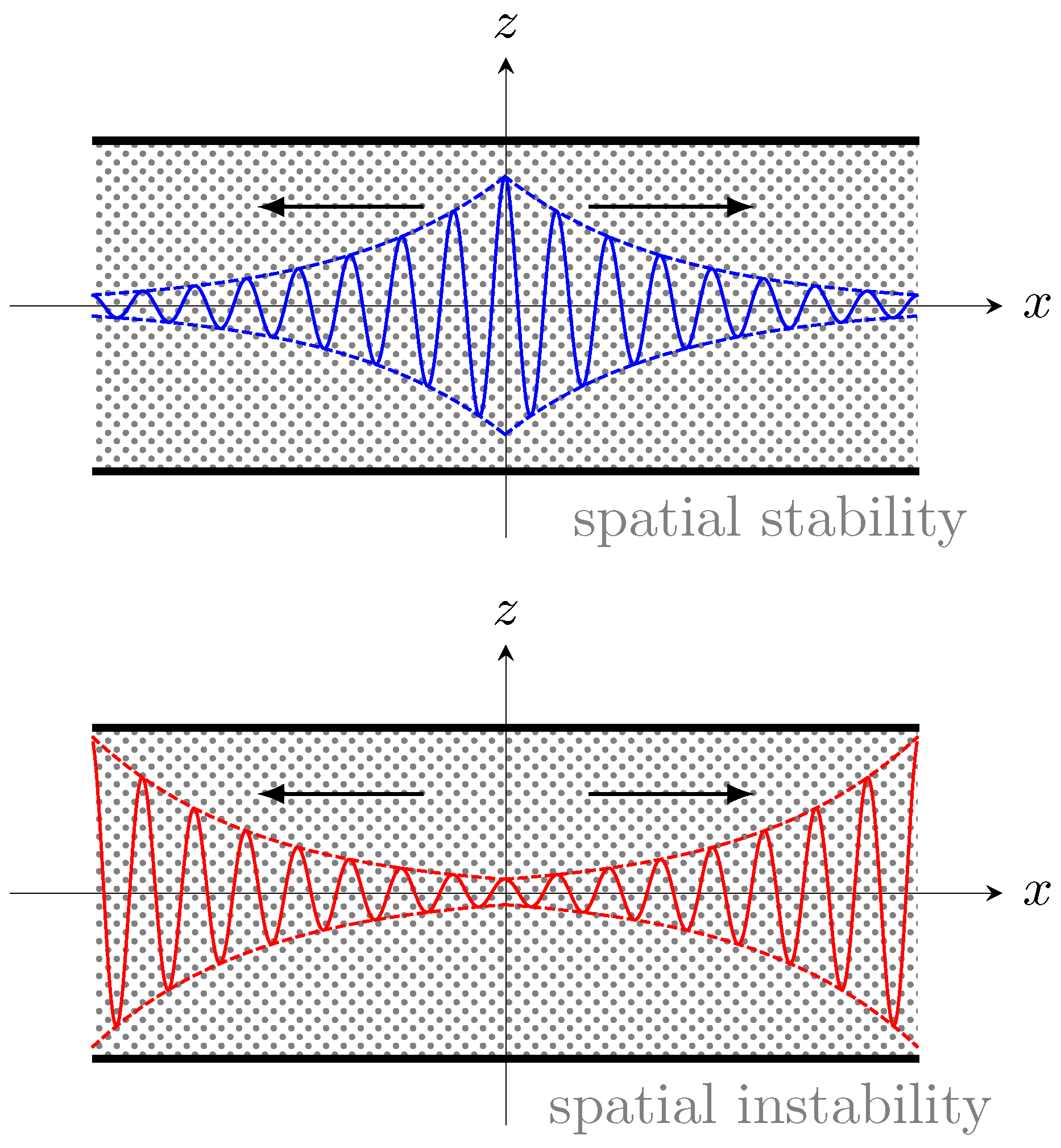
The rationale behind such definitions is that the time–periodic modes of the perturbations defined by Equations (19), (22) and (23) are stable when they are damped along their direction of propagation, which is determined by the sign of their phase velocity, $\omega /k$. On the other hand, the perturbation modes are spatially unstable when they are amplified along their direction of propagation. Without any loss of generality, one can fix $\omega >0$. Then, the sign of the phase velocity coincides with the sign of the imaginary part of $\eta \left(\omega \right)$, i.e., with the sign of k. A qualitative sketch of the concept described by Equations (28) and (29) is provided in Figure 1. Furthermore, the very special condition $\omega =0$ is discussed in Section 5 below.

An equivalent way to define spatial stability is by employing the argument function, $arg\left(a\right)$, whose values range within the interval $[-\pi ,\pi ]$, namely:

$$\begin{array}{c}\mathrm{spatial}\mathrm{stability}:-\frac{\pi }{2}<arg\left(\eta \left(\omega \right)\right)<0 \mathrm{or} \frac{\pi }{2}<arg\left(\eta \left(\omega \right)\right)<\pi ,\\ \mathrm{spatial}\mathrm{instability}:-\pi <arg\left(\eta \left(\omega \right)\right)<-\frac{\pi }{2} \mathrm{or} 0<arg\left(\eta \left(\omega \right)\right)<\frac{\pi }{2}.\end{array}$$

(30)

4.2. Parametric Conditions for Spatial Instability

One can first envisage the special case where $R=0$. From a physical viewpoint, such a case should not be prone to any kind of thermal instability. In fact, there is no thermal forcing coming from the boundary temperature difference as, with $R=0$, we have no temperature difference between the boundary planes, $z=0$ and $z=1$. This result is confirmed by Equations (22) and (27). In particular, Equations (27) yield:

$$\begin{array}{c}\begin{array}{c}\hfill {\eta }_1\left(\omega \right)=-{\eta }_2\left(\omega \right)=\sqrt{{\pi }^2-i\omega }, {\eta }_3\left(\omega \right)=-{\eta }_4\left(\omega \right)=\pi ,\end{array}\end{array}$$

(31)

in the case $R=0$.

On account of Equations (22), the roots ${\eta }_3\left(\omega \right)$ and ${\eta }_4\left(\omega \right)$ are unphysical as they yield a singularity of ${\tilde{\Psi }}_n(x,\omega )$, unless ${\tilde{\Theta }}_n(0,\omega )=0$. The latter condition is trivial as it yields vanishing perturbations. On the other hand, from Equation (31), one may conclude that the expressions for the roots ${\eta }_1\left(\omega \right)$ and ${\eta }_2\left(\omega \right)$ imply $sk=-\omega /2<0$, which yields spatial stability according to Equation (28).

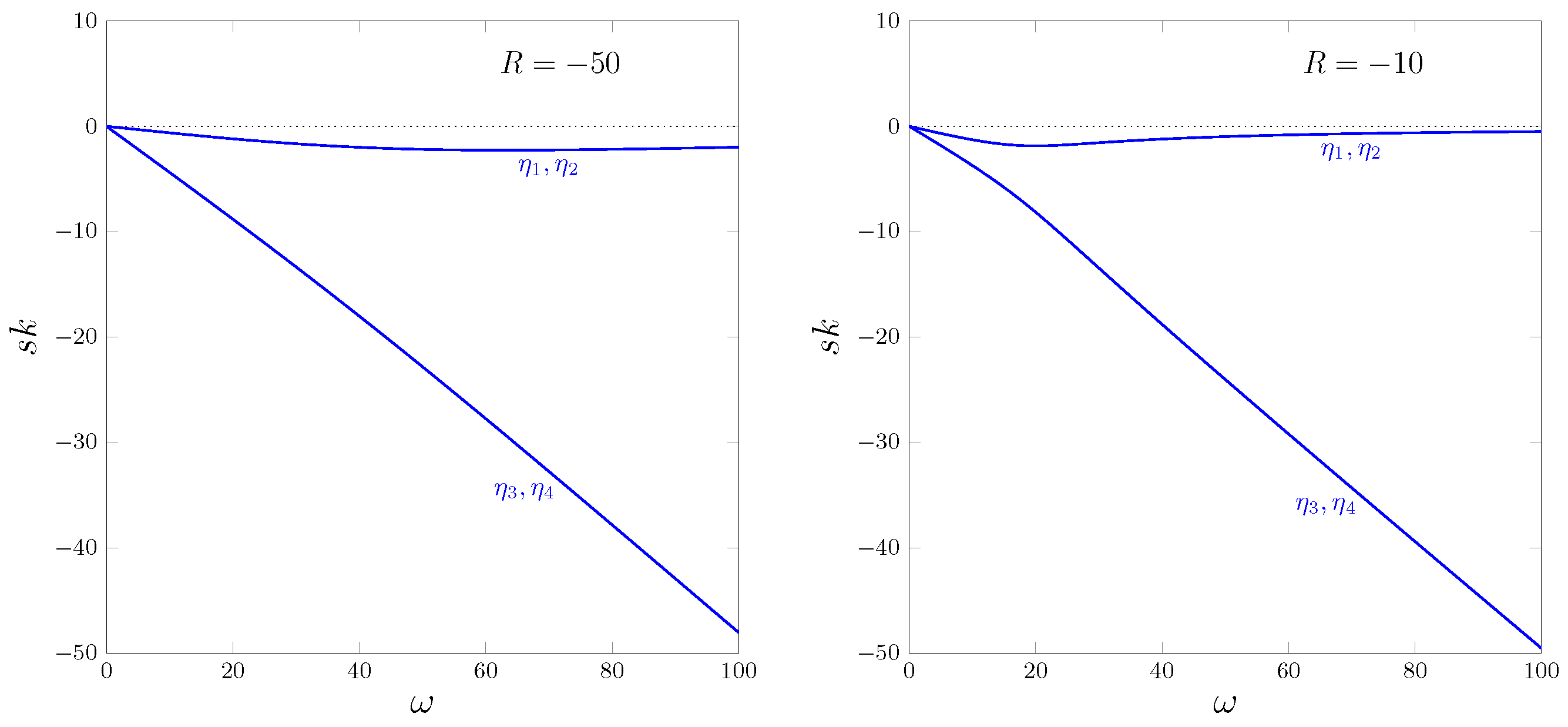
Figure 2 shows the plots of the product $sk$ for the branches $({\eta }_1,{\eta }_2)$ and for the branches $({\eta }_3,{\eta }_4)$, with two conditions of stable thermal stratification (heating–from–above), namely $R=-50$ and $R=-10$. The first remark is the obvious fact that $sk$ is identical for the root branches ${\eta }_1$ and ${\eta }_2$. In fact, the product $sk$ is the product between the real part and the imaginary part of $\eta$ and ${\eta }_2=-{\eta }_1$, on account of Equation (27). The same reasoning applies for the pair $({\eta }_3,{\eta }_4)$. A second feature suggested by Figure 2 is that, with $R<0$, no spatial instability is possible. This circumstance is a consequence of $sk$ being evidently negative in all cases illustrated in Figure 2. Hereafter, the blue colour is employed for the plots when the root branch $\eta$ corresponds to spatial stability, $sk<0$, while the red colour is used to denote spatial instability, $sk>0$. Let us note that the line corresponding to the pair $({\eta }_3,{\eta }_4)$ gradually, but slightly, deviates from the trend $sk=-\omega /2$ reported for the limiting case $R=0$.

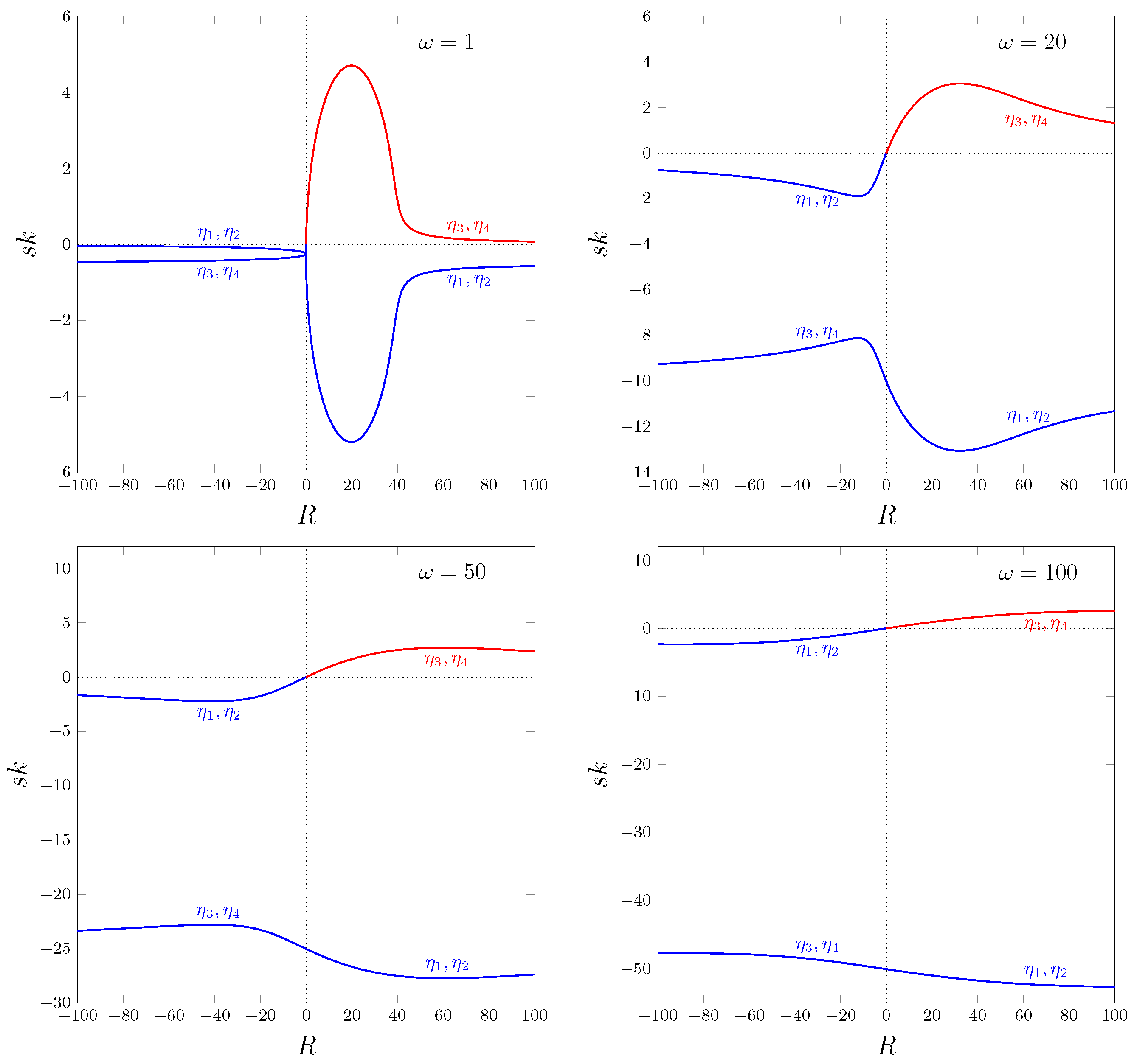
Figure 3 displays the product $sk$ versus R for the branch pairs $({\eta }_1,{\eta }_2)$ and $({\eta }_3,{\eta }_4)$. The plots are organised in four frames for $\omega$ values of $1,20,50$ and 100. The most important feature is the transition to spatial instability when $R>0$ for all the values of $\omega$ considered in Figure 3. The transition is evidently driven by the branches $({\eta }_3,{\eta }_4)$. One may notice the interchange between the branch pairs $({\eta }_1,{\eta }_2)$ and $({\eta }_3,{\eta }_4)$ while crossing the line $R=0$. Figure 3 further enforces the conclusion that no spatial instability is exploited with $R\le 0$. Thus, henceforth, the $R>0$ domain is focussed on, physically meaning an unstable thermal stratification (downward temperature gradient) in the basic conduction state.

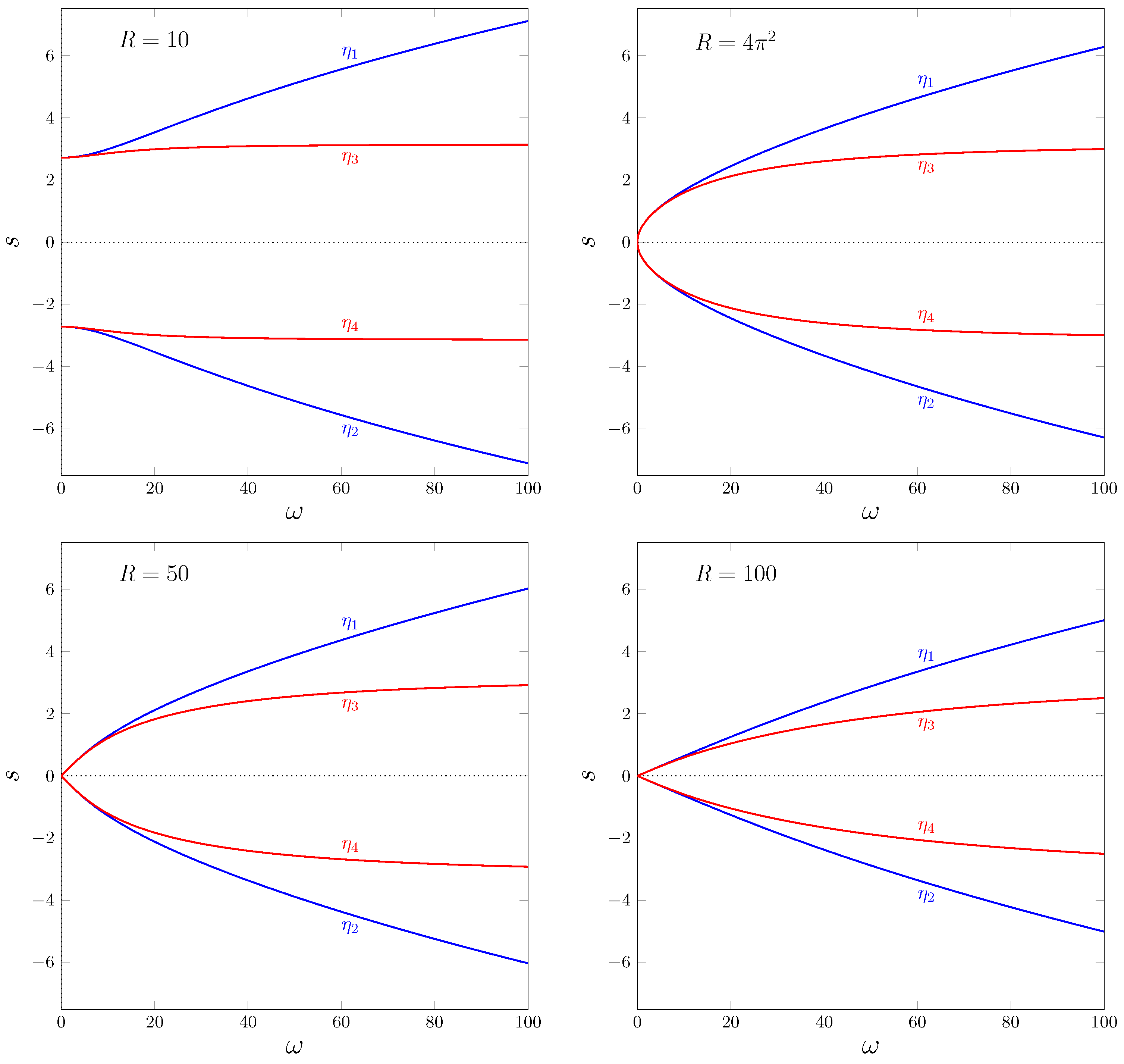
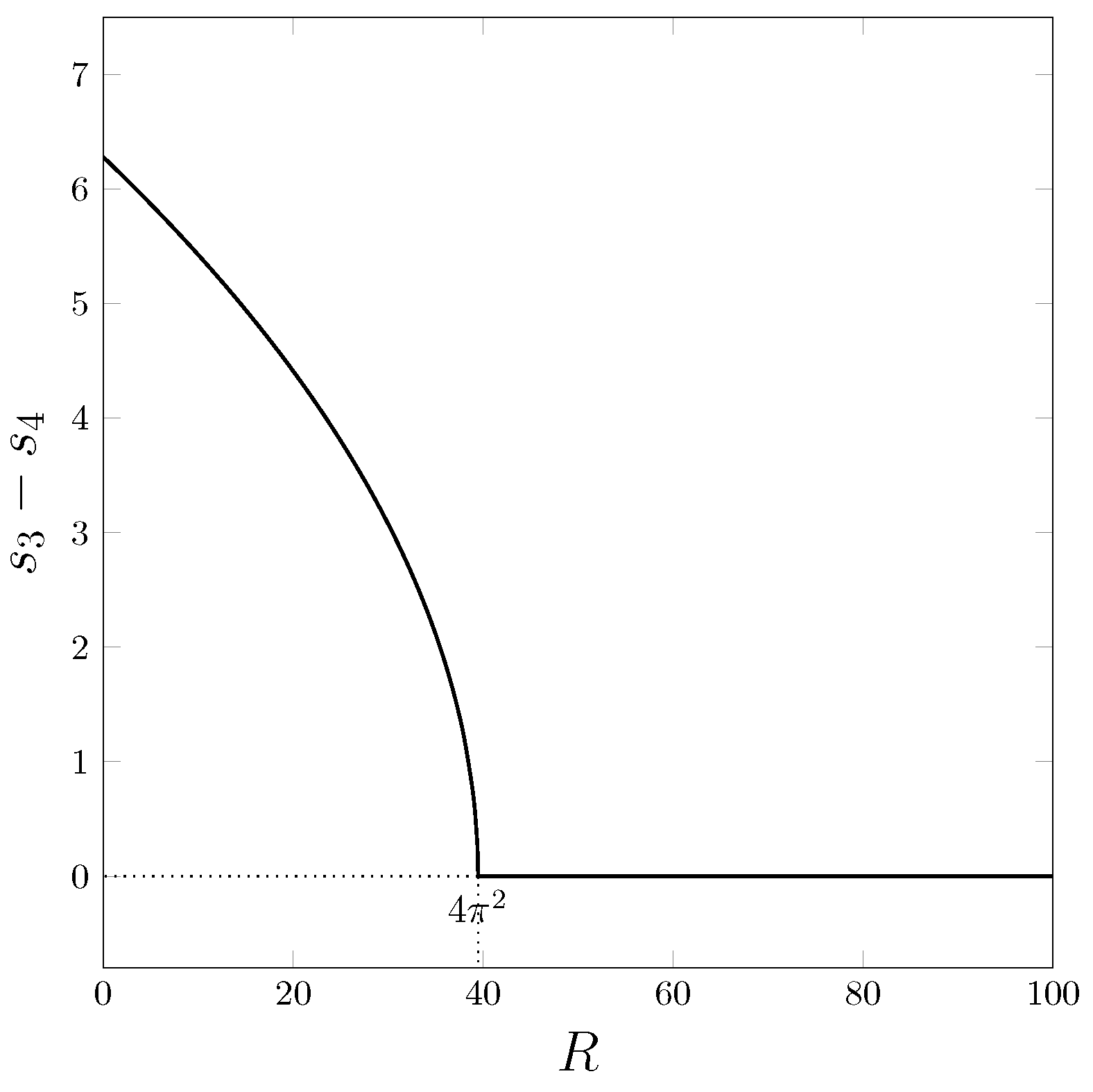
Figure 4 provides the plots of s versus $\omega$ for the four solution branches, given by Equation (27), with red lines denoting spatial instability, $sk>0$, and the blue lines indicating spatial stability, $sk<0$. The branches $({\eta }_3,{\eta }_4)$ are always spatially unstable with something special happening when $R=4{\pi }^2$ is approached from below. In fact, one can see that the frame with $R=10$ displays the branches $({\eta }_1,{\eta }_3)$ as completely detached from $({\eta }_2,{\eta }_4)$. When $R=10$ and $\omega \to 0$, the branches $({\eta }_1,{\eta }_3)$ approach a positive limit, while the branches $({\eta }_2,{\eta }_4)$ tend towards a negative value. With $R\ge 4{\pi }^2$, Figure 4 shows that the limit of s when $\omega \to 0$ is 0 for all the four branches. The distance at $\omega \to 0$ between the detached branch pairs, $({\eta }_1,{\eta }_3)$ and $({\eta }_2,{\eta }_4)$, decreases as R increases and becomes 0 when $R=4{\pi }^2$. This phenomenon is clearly illustrated in Figure 5, where the difference between the values of s for the branches ${\eta }_3$ and ${\eta }_4$ is shown (just the same plot can be obtained by considering ${\eta }_1$ and ${\eta }_2$, instead). It is noteworthy that $R=4{\pi }^2$ is the critical value for the onset of the convective instability, as it is recalled at the end of Section 3. However, here, this special value of R does not delimit the region of instability, as it happens with the spatially–periodic Fourier modes, discussed in Section 3. On the other hand, $R=4{\pi }^2$ is the minimum R such that the growth rate of the spatially unstable modes is 0 in the $\omega \to 0$ limit.

Another geometrical feature, displayed in Figure 4 and rigorously verified by employing Equation (26), is that, for $R=4{\pi }^2$, the condition $\omega \to 0$ is accomplished with

$$\begin{array}{c}\begin{array}{c}\hfill \underset{\omega \to 0}{lim}\eta =\pm i\pi \mathrm{and} \underset{\omega \to 0}{lim}\frac{\mathrm{d}\eta }{\mathrm{d}\omega }=\infty .\end{array}\end{array}$$

(32)

In particular, having an infinite $\mathrm{d}\eta /\mathrm{d}\omega$ means having a zero $\mathrm{d}\omega /\mathrm{d}\eta$. From the physical viewpoint, the latter is a zero group–velocity condition. This is a further situation where the spatial stability analysis mirrors, in a geometrical way, the classical stability analysis, carried out through spatially–periodic Fourier modes. In fact, the condition of zero group–velocity, or saddle–point condition, reflects the concept of absolute instability [13]. It is widely known that the Darcy–Bénard system displays the transition to absolute instability at critical conditions, $R=R_{\mathrm{c}}=4{\pi }^2$ with $k=k_{\mathrm{c}}=\pi$ [13]. As already pointed out above, within the spatial stability analysis, the value $R=R_{\mathrm{c}}=4{\pi }^2$ does not have the physical meaning of a threshold to instability (either convective or absolute), even if it displays significant geometrical characteristics. The analysis, presented in Section 5 just below, shows that there is more to say about the physical meaning of the neutral stability condition within the framework of the spatial stability analysis.

5. Stationary Spatially Developing Modes

The plot, given by Figure 5, refers to the limit $\omega \to 0$. However, the special case $\omega =0$ deserves a more thorough analysis. In fact, this case includes all the time–independent perturbations within the wider class of the spatially–developing modes defined in Section 4. Such special Fourier modes may display a different characterisation for their spatial stability/instability with respect to the inequalities (28) and (29).

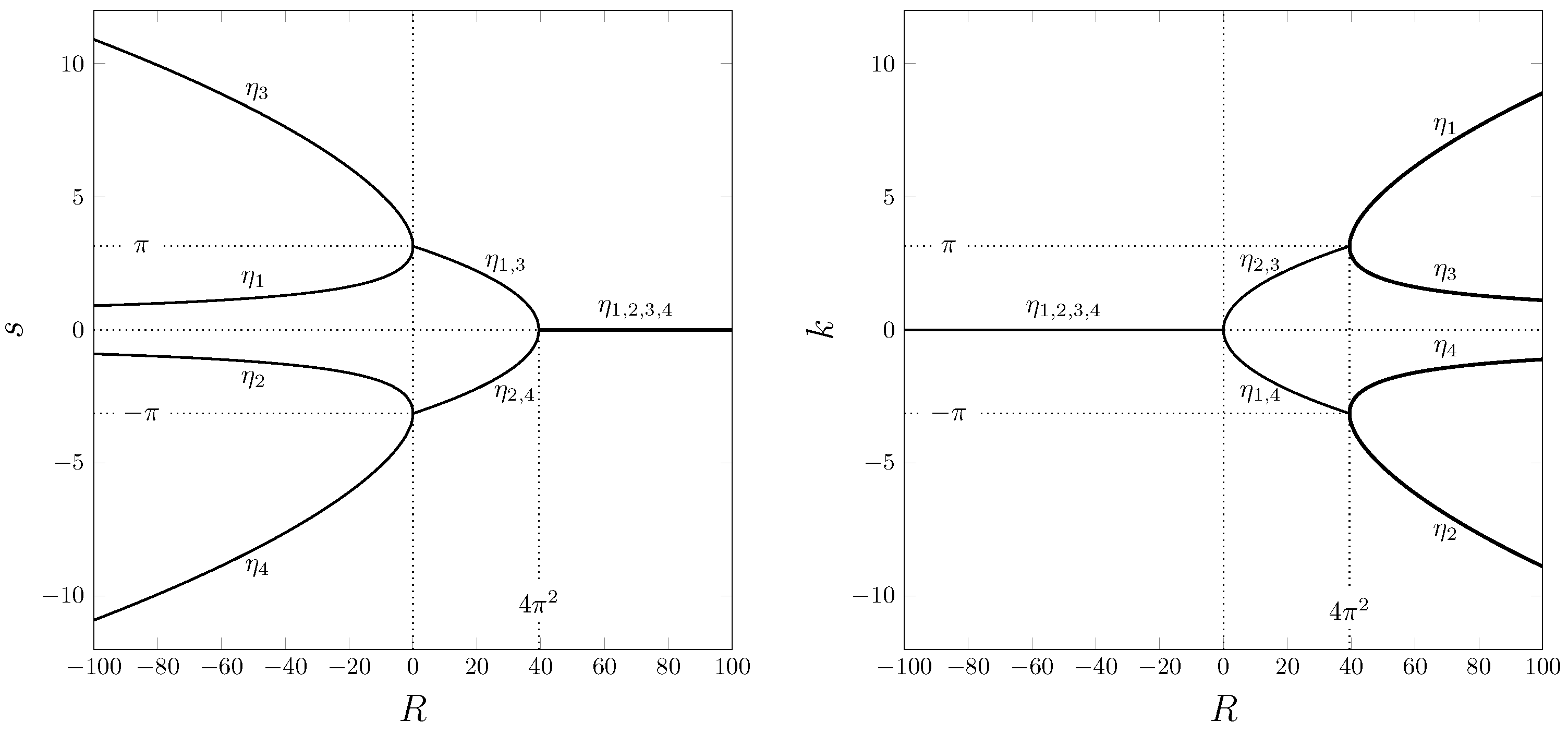
An illustration of the behaviour for the Fourier modes having $\omega =0$ is provided in Figure 6. The time–periodicity becomes time–independence with $\omega =0$, so that the entrance condition at $x=0$ is not oscillatory, but stationary. This circumstance entails a steady side heating or cooling mechanism through the cross–section $x=0$. Interestingly enough, this situation yields spatially–growing modes for every $R<4{\pi }^2$, either positive or negative. This phenomenon is shown in Figure 6. When $R<0$, the exponential growth with x, either in the positive or in the negative x directions, occurs for all the possible branches ${\eta }_j$, $j=1,2,3,4$. The vanishing k, when $R<0$, just means that the exponentially–growing modes do correspond to cells with infinite horizontal width. From the plots, displayed in Figure 6, one can see that the criterion for spatial stability/instability given by Equations (28) and (29) can be applied in the range $0<R<4{\pi }^2$. In fact, in this range, one has $sk<0$ (spatial stability) for the modes ${\eta }_1$ and ${\eta }_2$, while $sk>0$ (spatial instability) for the modes ${\eta }_3$ and ${\eta }_4$. The range $R\ge 4{\pi }^2$ is extremely important. Figure 6 reveals that $s=0$ in this range, so that one observes spatially–periodic modes. One can say that the range $R\ge 4{\pi }^2$ defines the intersection between the set of the spatially–periodic modes, used for the analysis in Section 3, and the set of the time–periodic modes, discussed in Section 4. In other words, the four thick lines, appearing with $R\ge 4{\pi }^2$ in the right–hand frame of Figure 6, form the neutral stability curve, defined by employing Equation (18) with $n=1$. This is perfectly consistent with the analysis, reported in Section 4, which clearly establishes how the neutral stability condition is obtained with a vanishing $\omega$ and with vanishing growth rates both in time and in space.

6. Further Insights into the Spatial Stability Analysis

Thus far, it has been demonstrated that the linear stability analysis of the Darcy–Bénard system can be carried out by employing either spatially–periodic Fourier modes or time–periodic Fourier modes. The former is the classical approach meant to focus on the time growth rate of the perturbations as the key parameter for establishing whether the basic state is stable or unstable. The latter has its focus on the spatial growth rate of the perturbations and on the concept of spatial instability occurring when the amplitude of the time–periodic Fourier modes grows in the spatial direction of propagation.

The two conceptions of instability are not equivalent as the instability to spatially–periodic modes is possible only with $R>4{\pi }^2$, while the instability to time–periodic modes is possible whenever $R>0$. Beyond their mathematical formulations and predictions, the difference between the two approaches to linear instability is grounded on diversified physical scenarios.

If one relies on the solution method, based on the Fourier transform, given by Equations (13) and (14), as well as on the expressions (16), it appears that one is tracing the evolution of a perturbation, defined by a function ${\widehat{\Theta }}_n(k,0)$. If such a function is processed through the Fourier inverse transform (14) and, then, it is substituted into the Fourier series (11), it becomes evident that, in fact, one prescribes an initial condition for the perturbation at time $t=0$. Thus, what one is doing is applying Lyapunov’s definition of stability/instability; see, e.g., Arnold [14]. This definition can be rephrased as follows: alter (slightly) an equilibrium state of a dynamical system and trace the evolution in time to demonstrate the stability/instability of that equilibrium state. The question is how an alteration in the initial state, at time $t=0$, affects the time evolution of a dynamical system. This is exactly the framework implied by Equations (13), (14) and (16).

The focus of spatial instability can be captured from Equations (19), (20) and (22). Here, one does not trace the evolution in time of an arbitrary initial condition fixed at $t=0$, but rather one describes the development in space of a condition set at a specified cross–section of the porous layer at $x=0$. If Lyapunov’s definition of the instability is based on the alteration of the initial condition at $t=0$, then one now conceives the instability, induced by an altered condition at $x=0$. The effects of such an alteration are measured by the development in space, i.e., along the x direction, of a signal prescribed at $x=0$. Hence, there are two distinct approaches for the test of the linear stability in a stationary fluid flow. Furthermore, the two types of stability test yield different outcomes, as it is mentioned above. The parametric ranges, expressed in terms of the Rayleigh number, for the instability to space–periodic Fourier modes and for the spatial instability, involving time–periodic Fourier modes, are different. Nevertheless, in both cases, one models the reaction of a basic flow to small–amplitude perturbations. The different outcomes are due to the different experimental procedures implied by the two schemes. Oversimplifying the description, spatially–periodic modes serve to measure the stability/instability on monitoring the time evolution of the perturbations. This task is meant to be achieved by observing the flow at a given spatial station, x. On the other hand, the time–periodic modes allow one to establish if the basic flow is stable/unstable by taking a snapshot of the whole flow domain at a given instant of time, t. If one takes into consideration the different experimental scenarios, implied by the two approaches, it is not surprising that the predicted parametric conditions for the instability are different.

Another remark is on the practical way to activate a time–periodic perturbation signal at a given cross–section, say at $x=0$. One can employ any device which induces a modulation in the time of the fluid temperature or pressure. For instance, it could be a vibrating element such as a membrane or an electric resistor subject to an alternating current (‘vibrating ribbons or harmonic point sources’, as suggested in Schmid and Henningson [12]). Due to the symmetry, the control volume for the experiment can be the half–domain $x>0$, without any loss of generality. We refer the reader to Chapter 7 in Schmid and Henningson [12] for further details on the physical meaning of the perturbations caused by a spatially–localised source.

Finally, let us comment on the four constants $C_j,$$j=1,\dots ,4$, employed in Equations (22). As it is already been pointed out, one has ${\sum }_{j=1}^4{C}_j=1$. This condition is meant to ensure the consistency for the expression of ${\tilde{\Theta }}_n(x,\omega )$ in Equations (22). An analogous constraint is formulated to ensure consistency for the expression of ${\tilde{\Psi }}_n(x,\omega )$ in Equations (22). Then:

$$\begin{array}{c}\begin{array}{c}\hfill \sum _{j=1}^4{C}_j=1, \sum _{j=1}^4\frac{C_j{\eta }_{j}R}{{\left(n\pi \right)}^2-{\eta }_j^2}=\frac{{\tilde{\Psi }}_n(0,\omega )}{{\tilde{\Theta }}_n(0,\omega )}.\end{array}\end{array}$$

(33)

Equation (33) is insufficient to determine uniquely the four constants $C_j$ for the functions ${\tilde{\Psi }}_n(0,\omega )$ and ${\tilde{\Theta }}_n(0,\omega )$. Two further extra conditions are to be set, constraining the derivative $\partial \mathbb{F}/\partial x$ at $x=0$. Such extra constraints depend on the nature of the time–periodic signal with angular frequency $\omega$, prescribed at $x=0$. One of the many possibilities is assuming symmetry conditions for the temperature and streamfunction perturbations, which yields $\partial \mathbb{F}/\partial x=0$ at $x=0$. If such constraints are implemented through Equations (22), Equation (33) is completed with:

$$\begin{array}{c}\begin{array}{c}\hfill \sum _{j=1}^4{C}_j{\eta }_j=0, \sum _{j=1}^4\frac{C_j{\eta }_j^{2}R}{{\left(n\pi \right)}^2-{\eta }_j^2}=0.\end{array}\end{array}$$

(34)

If the specification of the coefficients $C_j$ is requested to rigorously formulate the developing region problem for both $x>0$ and $x<0$, the actual experimental conditions may not yield accurately defined functions ${\tilde{\Psi }}_n(0,\omega )$, ${\tilde{\Theta }}_n(0,\omega )$ and constants $C_j$. One expects that, to some extent, an experimental setup of the Darcy–Bénard system likely shows up stochastic perturbation signals emerging at $x=0$ and developing in both the positive and negative x direction. The clue of the reasoning is that a random signal necessarily includes the most unstable modes, which turn out to dominate the flow development along x and determine its spatially stable/unstable nature.

7. Conclusions

In the present paper, the instability of the rest state in a horizontal porous layer with impermeable boundaries kept at different temperatures, known as Darcy–Bénard instability, is reconsidered. In particular, two different formulations of the linear analysis are compared. The first formulation is the classical one, where the reaction of the system to spatially–periodic Fourier modes, prescribed at the initial time $t=0$, is traced through its linear evolution. The second formulation leads to the concept of spatial stability/instability. In this case, the system response to the time–periodic Fourier modes, imposed at a given vertical cross–section, is tested. Conventionally, and without any loss of generality, the position, where the perturbation signal is imposed, is set to $x=0$. The main features, drawn from the comparison of such different formulations, are as follows.

• The spatial instability condition was formulated by adopting a Fourier transform in the time variable for the perturbations, thus giving rise to a complex growth rate parameter, $\eta$, along the x direction. The transition to spatial instability occurs when the product between the real part and the imaginary part of $\eta$ is positive.
• As it is widely known in the literature, the classical linear stability analysis, based on spatially–periodic Fourier modes, leads to the prediction of an unstable behaviour when the Rayleigh number, R, is larger than $4{\pi }^2$. On the other hand, the analysis involving time–periodic Fourier modes leads to the prediction of spatial instability whenever $R>0$, i.e., every time heat is supplied from below. In the special case of a zero angular frequency, $\omega =0$, spatially unstable modes exist also for $R<0$.
• Special geometrical features are displayed in the plots of the spatial growth rate, s = Re(η), versus the angular frequency, $\omega$, when $R=4{\pi }^2$. In particular, the two unstable branches of $\eta$, which are disconnected for $R<4{\pi }^2$, merge when $R=4{\pi }^2$. When this happens, a zero group–velocity condition is identified. However, such features are of purely mathematical nature and do not alter in any way the spatially unstable behaviour predicted for $R>0$, either smaller or larger than $4{\pi }^2$. In order to establish the physical meaning of the neutral stability condition within this framework, a special focus on the condition $\omega =0$ is provided.

The research reported is meant to be a starting point for further developments of the concept of spatial stability/instability for porous media saturated by a fluid. The tasks to be pursued in the future include the extension to the nonzero flow rate variant of the Darcy–Bénard problem, identifying the Prats instability problem [15]. Furthermore, the spatial instability concept can be pushed in the nonlinear domain where the constraint of small–amplitude perturbations is relaxed.

References

- Getling, A.V. Rayleigh–Bénard Convection: Structures and Dynamics; World Scientific: Singapore, 1998. [Google Scholar] [CrossRef]
- Drazin, P.G.; Reid, W.H. Hydrodynamic Stability; Cambridge University Press: Cambridge, UK, 2004. [Google Scholar] [CrossRef]
- Horton, C.W.; Rogers, F.T. Convection currents in a porous medium. J. Appl. Phys. 1945, 16, 367–370. [Google Scholar] [CrossRef]
- Lapwood, E.R. Convection of a fluid in a porous medium. Math. Proc. Camb. Philos. Soc. 1948, 44, 508–521. [Google Scholar] [CrossRef]
- Rees, D.A.S. The stability of Darcy–Bénard convection. In Handbook of Porous Media; Vafai, K., Hadim, H.A., Eds.; CRC Press: New York, NY, USA, 2000; Chapter 12; pp. 521–558. [Google Scholar]
- Tyvand, P.A. Onset of Rayleigh–Bénard convection in porous bodies. In Transport Phenomena in Porous Media II; Ingham, D.B., Pop, I., Eds.; Pergamon: New York, NY, USA, 2002; Chapter 4; pp. 82–112. [Google Scholar] [CrossRef]
- Straughan, B. Stability and Wave Motion in Porous Media; Springer: New York, NY, USA, 2008. [Google Scholar] [CrossRef]
- Nield, D.A.; Bejan, A. Convection in Porous Media; Springer: New York, NY, USA, 2017. [Google Scholar] [CrossRef]
- Vadasz, P. Instability and route to chaos in porous media convection. Fluids 2017, 2, 26. [Google Scholar] [CrossRef] [Green Version]
- Briggs, R.J. Electron–Stream Interaction with Plasmas; MIT Press: Cambridge, MA, USA, 1964. [Google Scholar] [CrossRef]
- Lingwood, R.J. On the Application of the Briggs’ and Steepest–Descent Methods to a Boundary–Layer Flow. Stud. Appl. Math. 1997, 98, 213–254. [Google Scholar] [CrossRef]
- Schmid, P.J.; Henningson, D.S. Stability and Transition in Shear Flows; Springer: New York, NY, USA, 2012. [Google Scholar] [CrossRef]
- Barletta, A. Routes to Absolute Instability in Porous Media; Springer: New York, NY, USA, 2019. [Google Scholar] [CrossRef]
- Arnold, V. Ordinary Differential Equations; Springer: New York, NY, USA, 1992. [Google Scholar]
- Prats, M. The effect of horizontal fluid flow on thermally induced convection currents in porous mediums. J. Geophys. Res. 1966, 71, 4835–4838. [Google Scholar] [CrossRef]
Figure 1.
A qualitative sketch of spatial stability (upper frame), and spatial instability (lower frame).
Figure 2.
The product of the porous layer spatial growth rate, s, and the wave number, k, versus the angular frequency, , for the values of the Rayleigh number, (left frame) and (right frame). Each frame contains plots made for the complex growth parameter pairs and , defined by Equations (27).
Figure 3.
The product versus R for (upper left), 20 (upper right), 50 (bottom left), and 100 (bottom right). Each frame contains plots for both branch pairs and . Red and blue lines denote the spatially unstable and stable modes, respectively.
Figure 4.
The rate s versus for (upper left), (upper right), 50 (bottom left), and 100 (bottom right). Each frame contains plots for four eigenvalue branches, , , and . Red and blue lines denote the spatially unstable and stable modes, respectively.
Figure 5.
The difference of the s values, calculated with and , versus R at .
Figure 6.
The growth rate, s (left frame), and the wave number, k (right frame), versus R for stationary modes, , for the four branches , and 4, given by Equations (27). Thicker lines identify the condition of neutral stability.
Publisher’s Note: MDPI stays neutral with regard to jurisdictional claims in published maps and institutional affiliations. |
© 2021 by the author. Licensee MDPI, Basel, Switzerland. This article is an open access article distributed under the terms and conditions of the Creative Commons Attribution (CC BY) license (https://creativecommons.org/licenses/by/4.0/).
Share and Cite
MDPI and ACS Style
Barletta, A. Spatially Developing Modes: The Darcy–Bénard Problem Revisited. Physics 2021, 3, 549-562. https://0-doi-org.brum.beds.ac.uk/10.3390/physics3030034
AMA Style
Barletta A. Spatially Developing Modes: The Darcy–Bénard Problem Revisited. Physics. 2021; 3(3):549-562. https://0-doi-org.brum.beds.ac.uk/10.3390/physics3030034
Chicago/Turabian StyleBarletta, Antonio. 2021. "Spatially Developing Modes: The Darcy–Bénard Problem Revisited" Physics 3, no. 3: 549-562. https://0-doi-org.brum.beds.ac.uk/10.3390/physics3030034