Effects of Quantum Metric Fluctuations on the Cosmological Evolution in Friedmann-Lemaitre-Robertson-Walker Geometries

1
School of Physics, Damghan University, Damghan 36716-41167, Iran
2
Department of Theoretical Physics, National Institute of Physics and Nuclear Engineering (IFIN-HH), 077125 Bucharest, Romania
3
Astronomical Observatory, 400487 Cluj-Napoca, Romania
4
Department of Physics, Babes-Bolyai University, 400084 Cluj-Napoca, Romania
5
School of Physics, Sun Yat-Sen University, Guangzhou 510275, China
*
Author to whom correspondence should be addressed.
Physics 2021, 3(3), 689-714; https://0-doi-org.brum.beds.ac.uk/10.3390/physics3030042
Submission received: 9 July 2021
/
Revised: 9 August 2021
/
Accepted: 11 August 2021
/
Published: 24 August 2021
(This article belongs to the Special Issue New Advances in Quantum Geometry)
Abstract
:In this paper, the effects of the quantum metric fluctuations on the background cosmological dynamics of the universe are considered. To describe the quantum effects, the metric is assumed to be given by the sum of a classical component and a fluctuating component of quantum origin . At the classical level, the Einstein gravitational field equations are equivalent to a modified gravity theory, containing a non-minimal coupling between matter and geometry. The gravitational dynamics is determined by the expectation value of the fluctuating quantum correction term, which can be expressed in terms of an arbitrary tensor . To fix the functional form of the fluctuation tensor, the Newtonian limit of the theory is considered, from which the generalized Poisson equation is derived. The compatibility of the Newtonian limit with the Solar System tests allows us to fix the form of . Using these observationally consistent forms of , the generalized Friedmann equations are obtained in the presence of quantum fluctuations of the metric for the case of a flat homogeneous and isotropic geometry. The corresponding cosmological models are analyzed using both analytical and numerical method. One finds that a large variety of cosmological models can be formulated. Depending on the numerical values of the model parameters, both accelerating and decelerating behaviors can be obtained. The obtained results are compared with the standard CDM ( Cold Dark Matter) model.
1. Introduction
General relativity and quantum mechanics are the basic, and widely accepted, branches of theoretical physics, confirmed by a large number of experiments and observations. In particular, general relativity, a theory of gravity [1,2,3] is a typical example of a physical theory with a very beautiful geometric structure. Moreover, it is one of the very successful existing physical theories, with its predictions being confirmed in the past one hundred years with a high degree of accuracy [4,5,6]. In addition to the classical tests of general relativity performed at the Solar System level, recently two other fundamental predictions of general relativity, the existence of the gravitational waves, and the existence of black holes, have also been confirmed [7,8].
Despite the remarkable achievements of both quantum mechanics and general relativity, it had been known for a long time that these two fundamental theories of physics cannot be unified, and they seem to be incompatible with each other. The first in depth analysis of the possibility of the unification of quantum mechanics and general relativity was performed by Bronstein [9], whose analysis indicated the existence of an essential difference between quantum theory and the quantum theory of the gravitational field based on general relativity. These early results already pointed out to the fundamental difficulty of unifying quantum theory and general relativity. Even after almost ninety years of intensive effort the task of building a quantum theory of gravity is still unfulfilled, remaining an open assignment for modern theoretical physics. There are many approaches to quantum gravity, and for an introduction to the field, see, e.g., [10,11].
One possible avenue for the quantization of gravity would be its reformulation as a gauge theory, an approach pioneered in [12], and further developed in [13,14,15,16,17]. Another attempt to a quantum theory of gravity was initiated in [18,19,20], and it is based on the rewriting of the Hilbert-Einstein action in terms of a spin connection and a set of tetrads. Since both the tetrads and the spin connection are vector fields, the theory of gravitation can be reformulated as a vector gauge theory.
However, from a fundamental physical point of view, such an approach is not satisfactory, since in the case of gravitation the principles of equivalence and of the general covariance are more important than the gauge principle, on which the standard model of particle physics and its extensions are based [21]. Moreover, the theory is still based on the standard Hilbert-Einstein action, and it is not clear at this moment if it can be quantized. Various other approaches have been proposed for the quantization of the gravitational field in [22,23,24,25,26,27,28,29].
A possible way of dealing with the problem of the quantization of gravity, and a first step in this direction, is to assume that the matter fields are quantized, and that evolve in a classical spacetime, described by a metric , where the indices, denoted by Greek letters, take on the values 0, 1, 2, 3. There is an important difference in this case as compared to the evolution in a Minkowski spacetime, in the sense that in general there is no preferred vacuum state for the fields. Consequently, particle creation effects naturally take place. In semiclassical gravity the gravitational field is described classically, using the Hilbert-Einstein action, , where R denotes the Ricci scalar, is the gravitational coupling constant, g is the determinant of the metric tensor, and x represents the time () and space (, , ) coordinates. Hence, in semiclassical gravity quantum matter is coupled to the gravitational field via the semiclassical Einstein equations,
where G is the Newtonian constant of gravitation, c is the speed of light, and is the quantum operator associated with .
The above equations are obtained by replacing in the Einstein gravitational field equations , the classical matter energy-momentum tensor by the expectation value, , in an arbitrary quantum state of the quantum operator associated with . The semiclassical approach to quantum gravity was proposed initially in [30,31], and it has been further developed and discussed in [32,33,34,35,36,37,38,39,40,41,42,43,44].
From Equation (1) it follows that the matter energy-momentum tensor is obtained in the classical limit by assuming . The semiclassical Einstein Equation (1) can also be derived from the variational principle [35], where is the standard Hilbert-Einstein general relativistic classical action of the gravitational field, while the second component of the total action, generated by quantum effects, is given by:
where is a Lagrange multiplier, while is the Hamilton operator of matter.
A more general pathway to semiclassical gravity was introduced in [35]. It is essentially based on the idea of the introduction of a nonminimal coupling between the classical Ricci scalar R, and the quantized matter fields. Specifically, one can introduce in the total action a term containing the quantum matter-geometry coupling with the simple form: . In the coupling term, F and f denote some arbitrary functions, while denotes the average value of a function over the quantum fields. Then, the effective semiclassical Einstein equations are given by [35]:
The semi-classical effective gravitational model described by Equation (2) has one important consequence, namely, that the mean value of the matter energy-momentum tensor is not conserved directly, since generally . Thus, the theoretical model described by Equation (7) can be interpreted theoretically as describing a process of particle production that is the direct result of an energy removal from geometry to matter.
An alternative method for the quantization of classical physical structures is the stochastic quantization method, introduced initially in [45]. In this approach to quantization of the classical systems the quantum fluctuations are characterized with the help of the stochastic Langevin equation. The stochastic quantization method goes back to the study initiated in [46], in which the Schrödinger equation was from the classical dynamics obtained using stochastic methods. However, the rigorous formulation of the stochastic quantization method was presented in [45]. In stochastic quantization the quantum mechanical picture of physical processes is constructed through the limit, with respect to a fictitious time variable t, of a hypothetical higher-dimensional stochastic process, assumed to be described by a Langevin type equation. For the early advancements in stochastic quantization theory see [47,48]. For the gravitational field the stochastic quantization procedure was introduced in [49,50], by assuming that the classical metric tensor obeys the covariant stochastic Langevin equation, given by [49]:
where is a stochastic source term, is a parameter, and a dot denotes the derivative with respect to . For recent discussions on the stochastic quantization of gravity see [35]. For alternative Einstein-Langevin type equations, see, e.g., [51,52].
The quantum fluctuations of the space time are assumed to play an important role in the quantum description of gravity. In fact, long time ago, it was suggested that due to the Heisenberg uncertainty principle over extremely small distances and sufficiently small intervals of time, the geometry of spacetime may fluctuate [53,54]. The quantum fluctuations of the spacetime could be large enough to induce important deviations from the smooth spacetime one experiences at macroscopic scales, and giving spacetime a “foamy” character [53,54].
Quantum fluctuations play a central role in the alternative semi-classical description of quantum gravity, introduced in [55]. In this approach to quantum gravity, the quantized metric is assumed to have two components, and is given as the sum of classical and quantum terms. After performing this decomposition, the quantized Einstein equations can be approximated at the classical level by a modified gravity theory that includes a nonminimal coupling between matter and geometry. After introducing some natural hypotheses for the two-points expectation value of the product of the fluctuating quantum metric, one can obtain the effective semiclassical gravitational and scalar field Lagrangians [56]. For a vanishing expectation value of the first-order terms of the metric, the second order corrections can also be calculated. The second order quantum corrections also lead to a modified gravity theory.
The gravitational field equations and the modified conservation laws were obtained within the framework of the fluctuating metric approach in [57]. It was also shown that due to the quantum fluctuations a bouncing universe model can be constructed. Moreover, in a dark energy dominated phase, a decelerated expansionary cosmological evolution is also possible. Gravitational models with fluctuating metric were studied in [58,59,60]. In particular, after expressing generally the expectation value of the quantum correction in the form of a general second order tensor, in [61] the effective gravitational field equations at the classical level have been derived in a general formulation. Cosmological models with the quantum correction tensor given by the coupling of a scalar function and of a scalar field to the metric tensor, as well as by a quantum term proportional to the ordinary matter energy-momentum tensor, were analyzed. These models can describe the present day accelerated expansion of the universe.
One of the important implications of the gravitational theories with fluctuating quantum type metric is that they typically lead to modified gravity models in the presence of a geometry-matter coupling. Such theoretical models have been proposed already in the framework of standard classical general relativity as viable explanations of the recent cosmological observations that have determined a fundamental change in our comprehension of the universe. Very precise and detailed astronomical and astrophysical observations indicate that recently the universe experienced a transition from deceleration to an accelerating, de Sitter type regime [62,63,64,65,66,67]. These cosmological observations are usually interpreted through the postulation of the existence of a dominant constituent of the universe, called dark energy, and whose presence can give a reason for all recent cosmological observations [68,69]. However, a second major constituent, called dark matter, is also required to fully explain the observations [70,71].
On the other hand, one cannot reject a priori the possibility that the two major constituents of the universe, dark energy (usually modelled as a cosmological constant [72,73]), and dark matter, could be explained as a common and basic property of a generalized gravity theory that goes ahead of standard general relativity, and its Hilbert-Einstein variational formulation. Many extended gravity theories, modifying and generalizing Einstein’s general relativity have been suggested recently. One of the first extensions of general relativity is represented by the gravity theory, with gravitational action of the form [74,75,76,77,78,79], where denotes the matter Lagrangian density. gravity generalizes only the geometric part of the gravitational action, and thus it ignores the profound role the matter Lagrangian could have [80]. Moreover, theory is still based on a minimal coupling between geometry and matter.
Extended gravity theories with arbitrary matter-geometry couplings were introduced initially in [81,82,83,84] in the form of the -modified gravity theory, with the gravitational action given by . In this approach, geometry becomes equivalent with matter, and thus matter plays a more important role in describing the properties of space-time as the one ascribed to it in standard general relativity.
The gravity theory introduces an other type of matter-geometry coupling, with the gravitational action given by [85,86]. Hence, in theory matter and geometry are coupled through the trace T of the energy-momentum tensor. Many other gravitational theories with geometry-matter couplings have been proposed and studied widely up to now. Among them are the gravity theory [87,88], the hybrid metric-Palatini gravity theory, with representing the Ricci scalar, formed with the help of a connection not depending on the metric, such as in the case of the Levi-Civita connection [89,90,91], the Weyl-Cartan-Weitzenböck (WCW) theory [92], and the modified gravity theory [93,94], where Q is the non-metricity.
Modified gravity theories in which the torsion scalar couples nonminimally to the trace T of the matter energy-momentum tensor are called gravity theories. These types of theories have also been extensively investigated [95]. In [96] theories with higher derivative matter fields were considered in detail. Extensive reviews of the , , and hybrid-metric-Palatini type gravity theories can be found in [97,98].
All gravitational theories with matter-geometry coupling have the curious particularity implying that the four-divergence of the matter energy-momentum tensor does not vanish generally, so that . This non-conservation of can be understood from a physical point of view using the formalism of the thermodynamics of open systems [86,99,100]. Hence, in these gravitational theories, one can presume that the energy and momentum balance equations describe irreversible particle creation processes. Thus, the non-conservation of indicates an irreversible matter and energy transfer from the gravitational field to the newly produced particles.
The creation of particles from the cosmological vacuum is one of the significant predictions of the quantum field theory in curved space-times [101,102,103,104,105]. Quantum field theoretical approaches to gravity lead naturally to particles creation processes, and they play an essential role in the understanding of the foundations of the theory. In the expanding Friedmann-Lemaitre-Robertson-Walker geometry, quantum field theory in curved spacetimes predict that quanta of the minimally coupled scalar field are produced permanently from the cosmological vacuum [105,106,107].
Hence, the presence at the theoretical level of the particle creation processes in both quantum theories of gravity in curved space-times and in modified gravity theories with geometry-matter coupling suggests that a deep relationship may exist between these two, seemingly distinct physical theories. In fact, such a relationship was already obtained in [57], where it was found that in the nonperturbative approach for the quantization of the metric, as introduced in [55,56,58], as a consequence of the fluctuations of the spacetime, a specific type gravitational model naturally emerges. The Lagrangian density of the theory is given by:
where is a constant. This result suggests that a phenomenological description of quantum mechanical particle production processes may be possible in the or type theories. Such a semiclassical approach could lead to a better understanding of the quantum processes describing matter creation through an equivalent semi-classical description essentially involving the coupling between geometry and matter.
It is the main goal of the present study to further investigate the physical, astrophysical and cosmological implications of the effective modified gravitational theories induced by the quantum fluctuations of the space-time metric, as developed in [55,56,57,58], and further considered in [61]. Let us start the analysis by assuming that within a semiclassical approximation the quantized gravitational field can be described by a quantum metric, which can be decomposed into two terms. They are the classical, and a stochastic fluctuating component of quantum origin. Hence, the metric is obtained as the sum of these two components. As a result of this decomposition, the Einstein quantum gravity leads to an effective gravitational theory, analogous to the modified gravity models with a nonminimal coupling between geometry and matter, which have been already analyzed in [81,85,87]. Hence, it is proposed that a quantum gravitational theory can be illustrated within a semiclassical approximation.
To obtain some specific predictions from the effective gravitational theory obtained from the fluctuating quantum metric, one has to introduce the assumption that the expectation value of the quantum correction tensor can be constructed from the metric, and from the thermodynamic quantities describing the ordinary matter content of the universe. In the present approach, the functional form of is fixed using the Newtonian limit of the theory. By assuming that can be represented as a linear combination of the metric, the Ricci tensor and the matter energy-momentum tensor, with the coefficients depending on the Ricci scalar R and on T, one derives first the Poisson equation in the presence of quantum fluctuations. Then, the functional form of is determined by requiring compatibility with the Solar System observations. Hence, from the Newtonian limit, one obtains the form of that satisfies all the Solar System constraints. Then, the cosmological implications of the obtained forms of is investigated by considering four distinct cosmological scenarios.
The present paper is organized as follows. In Section 2, the field equations, induced by the quantum fluctuations of the metric, are obtained in general form using the variational principle. The modified Poisson equation for this modified gravity theory is also derived, and a set of constraints on the model parameters are obtained. The general cosmological implications of the modified gravity theories in the presence of quantum metric fluctuations are discussed in Section 3. Several cosmological models, obtained for different choices of the fluctuation tensor are investigated in detail in Section 4, using numerical methods. The results are discussed and concluded in Section 5. The full form of the generalized Friedmann equations obtained in the presence of a fluctuation tensor satisfying the Solar System tests are presented in Appendix A. In the present paper, a system of units with the speed of light is used.
2. Quantum Metric Fluctuations Induced Gravitational Field Equations
Quantum mechanics is a very successful fundamental theory of physics, providing an excellent description of atoms, molecules, elementary particles, and classical fields, excluding gravitation. The quantum mechanical approach requires that all physical quantities must be described by operators acting in a Hilbert space. If gravity can also be described quantum mechanically, then it follows that all geometrical quantities characterizing the gravitational field must be quantized by identifying them with some suitably chosen operators. Hence, in one would like to construct a proper quantum theory of the gravitational field, Einstein’s gravitational field equations must take an operator form, given by [55,56,58]:
This formal representation corresponds to the non-perturbative quantum approach. Useful physical information should be extracted from the quantum Einstein operator equations by taking their average values over all possible products of the quantum metric operators [55,56,58]. By introducing the Green functions, , of the quantized gravitational field, the exact quantum approach to gravity implies to obtain the solutions of the infinite system of operator equations,
In the above equations, represents the quantum state associated with the gravitational field. As this moment it is important to point out that may not necessarily represent the ordinary vacuum state of the standard quantum field theory in curved spacetimes. Unfortunately, no exact analytical solutions of the operator equations for the gravitational Green functions are known so far, and it seems that it may not be possible to obtain their solutions analytically. Therefore, the investigation of the physical implications of the quantum gravity models needs to use approximate methods [55,56,57,58]. A possible suggestion for the study of quantum gravity was presented in [55]. This approximations is based on the decomposition of the quantum metric operator, , into the sum of two components. The first one is the average of the classical metric , while the second one corresponds to the fluctuating component, . Hence, in this approach, the quantum metric reads:
Moreover, at this moment another approximation is introduced. Let us suppose that the average value of the fluctuating part of the metric, which is typically of a quantum nature, can be represented with the help of a classical tensor quantity , so that:
Hence, in the present approach, the classical and quantum degrees of freedom are coupled using an expectation value. When such a coupling occurs there will be no effects of quantum fluctuations on the classical system [108]. Generally, in its Copenhagen interpretation, for a microscopic physical system quantum mechanics gives the amplitudes for many different states at a given time t. In the presence of quantum fluctuations, due to the interactions at later times, one cannot obtain a unique set of values of the physical or geometric quantities, but only a probability distribution for the different states. On the other hand, in the present semiclassical approach to quantum gravity, there is a unique solution for the metric, once the initial data for the metric and wave function are known. Hence, in this sense, quantum fluctuations do not influence the evolution of the metric. Moreover, if the metric and the initial state are homogeneous and isotropic, it follows that these symmetries are preserved by the dynamics of the gravitating system. Hence, one arrives at the important physical result that quantum fluctuations do not generate spatial variations in the energy-momentum tensor, or in the gravitational field itself [108]. Therefore, the character of the cosmological evolution is not influenced by the presence of the quantum fluctuations.
Then, by ignoring higher order fluctuations, the Lagrangian of the gravitational theories that also considers the consequences of the quantum fluctuations can be obtained as [55]:
where , denotes the (quantized) Lagrangian of the gravitational field, is the matter Lagrangian, while is the energy-momentum tensor of the classical matter, defined as:
Therefore, in the present approach to quantum gravity, the analysis starts with the full system of the gravitational field equations in operator form. As a next step, the metric is decomposed into two terms, the first being the classical part, while the second term a stochastic fluctuating part. Thus, one obtains an effective semiclassical theory of gravity, completely described in terms of classical concepts and quantities. However, in this approach one cannot obtain the functional form of , the important quantum perturbation tensor, from the first principles. Therefore, the form of must be chosen from physical considerations.
The first-order corrected quantum Lagrangian (7) leads to the following general gravitational field equations:
where and . Moreover, is either or . On the other hand, may represent an operator, an algebraic tensor, or their combination. One can also obtain the conservation of the energy-momentum tensor:
One can see immediately that in the case of a vanishing , the matter energy-momentum tensor becomes a conserved quantity.
The Modified Poisson Equation
The tensor is a second order symmetric tensor, and it is responsible for the quantum corrections of the quantum metric tensor. In general, it can be proportional to any classical second rank tensor existing in general relativity. However, one may assume that it is a function of the geometric and thermodynamic quantities describing a gravitational system. Moreover, in the following it is assumed that has a linear dependence on these quantities, and hence, a general form of the tensor is:
where , , are general functions of the classical Ricci scalar R, and of the trace T of the energy-momentum tensor. We would like to emphasize that here the Latin letters do not denote the spatial coordinates. The background solution for the Minkowski space time of Equation (9) is , where is a constant.
To obtain the Newtonian limit of this model, one perturbs the field equations around the Minkowski space time up to first order in perturbed quantities. Then, the perturbed metric is represented in the Newtonian gauge:
where and are general functions of spatial coordinates and the indices, denoted by Latin letters, stay for spatial coordinates. In the first order of perturbations the Lagrangian of the matter field and its energy-momentum tensor takes the form:
where is the matter energy-density.
One should note that since the Newtonian limit of the model is considered, the matter is assumed to be non-relativistic with the thermodynamic pressure . In the first order of approximation of Equation (11), the coefficients , appearing in , contribute up to the linear order in R and T which gives:
where and are constants. The term reproduce the Einstein-Hilbert action. The term containing is redundant because the same terms are generated by and , respectively. Hence, in the following, Equation (14) is considered with .
With these assumptions, the first-order off-diagonal components of Equation (9) yield:
Using the above equation, the components of Equation (9) will be satisfied in first order, while the component becomes:
The above equation differs from the Poisson equation for the gravitational potential due to the presence of the first and second terms in the left-hand side. The generalized Poisson equation provides a very powerful theoretical tool for investigating the consistency of modified gravity models. For example, in [109] the modified Poisson equations for -gravity were obtained in the form of the system:
where , and and are the two metric potentials, as introduced in Equation (12). By a prime we have denoted the derivative with respect to the argument of the function.
After eliminating the higher-order terms, one can recover the standard Poisson equation of general relativity. As an application of the modified Poisson equation, used together with the collisionless Boltzmann equation, the Jeans stability criterion in gravity was investigated in [109], by considering a small perturbation from the equilibrium and linearizing the field equations. From the performed analysis, unstable modes, not present in the standard Jeans analysis, were obtained.
To be compatible with the Solar System observations, the coefficients of these two terms should be very small. In the following, we set . Additionally, one should have , a condition that can be safely satisfied for .
As a result, the form of the tensor up to the linear order is obtained:
In Section 3, several classes of cosmological solutions of the quantum metric fluctuations, induced modified gravity theory with the above form for the tensor , are considered.
3. Cosmological Models with Quantum Metric Fluctuations
In this Section, the cosmological implications of the extended gravity models, obtained from the effective approach to quantized gravity introduced in the previous sections, are investigated. After presenting the basic geometrical and physical assumptions, defining the basic parameters used for the characterization of the cosmological models, one considers four specific models of the universe, obtained by adopting some specific functional forms for the fluctuation tensor .
3.1. Metric and Field Equations
In the following, for the metric of the universe, we adopt the homogeneous and isotropic flat Friedmann-Lemaitre-Robertson-Walker line element [110],
where the scale factor is a function of the cosmological time only. At this moment the Hubble function H, defined as , is introduced. Moreover, we assume that the matter content of the universe consists of a perfect fluid, characterized by two thermodynamic quantities only, the energy density , and the thermodynamic pressure p. Then the matter energy-momentum tensor is given by:
For the matter equation of state, let us adopt the linear barotropic equation of state , where is a constant. For the choice of , as given by Equation (19), the cosmological field Equation (9), representing the generalized Friedmann equations, are:
and
where and are given in Appendix A.
To specify the accelerating/decelerating type of the cosmological expansion, one uses the deceleration parameter q defined as:
Using Equations (22) and (23):
where and . A dust universe reaches the marginally accelerating state with once the condition is satisfied. The general condition for accelerating expansion can be formulated as .
To simplify the mathematical formalism, a set of dimensionless parameters
is introduced:
where is the current value of the Hubble parameter.
To expedite the testing of the theoretical predictions of the model with the cosmological observations, one introduces, instead of the cosmological time variable t, as independent variable the redshift z, defined as:
where one normalizes the scale factor a by imposing the condition that its present-day value is one, . Hence, one replaces in all cosmological evolution equations the derivatives with respect to the cosmological time t with the derivatives with respect to the redshift z, so that
As a function of the cosmological redshift, the deceleration parameter is obtained as:
In what follows, the cosmological evolution of the universe filled with non-relativistic matter with for four independent choices of the fluctuation tensor is considered.
3.2. The Standard CDM Model
In this investigation, we also include a comparison of the behavior of the physical and geometric cosmological quantities obtained from the present version of the modified gravity induced by the quantum metric fluctuations with the standard CDM (Cold Dark Matter) model, where is the cosmological constant.
The recent results of the study of the cosmic microwave background radiation by the Planck satellite has provided high precision cosmological data [62,111,112,113,114,115,116,117]. In the following, the simplifying assumption that the present day universe consists mostly of dust matter, with negligible pressure, is adopted. Hence, the energy conservation equation, , of standard general relativity gives for the variation of the matter energy density the expression, , where is the present-day matter density. As a function of the scale factor the time variation of the Hubble function is obtained in the form [115]:
where , , and denote the density parameters of the baryonic matter, the cold (pressureless) dark matter, and the dark energy (described by a cosmological constant), respectively. The three density parameters satisfy the important relation , indicating that the geometry of the universe is flat.
As a function of the redshift the dimensionless form of the Hubble function is obtained as:
For the deceleration parameter, as a function of the redshift, then one finds
In this study, for the density parameters, the numerical values , , and [115] are are adopted, as obtained from the Planck data. For the total matter density parameter, , the value is taken. The present day value of the deceleration parameter is given by , corresponding to an accelerating expansion of the universe [115,116]. The dependence of the dimensionless matter density on the redshift is given, in the standard CDM cosmological model, by [115,116].
4. Specific Cosmological Models
Here, a few particular cosmological models are investigated, in which for the fluctuation tensor some particular forms are adopted, which follow from the general representation (19). These specific forms of are obtained by fixing the values of the arbitrary coefficients , and , .
4.1.
As a first example of a cosmological model in the modified gravity theory induced by the metric fluctuations, one considers that the tensor is proportional to the Ricci tensor:
This form of is obtained by taking in Equation (19). To obtain a dimensionless form of the cosmological evolution equations, the dimensionless parameters and are introduced:
In terms of redshift z, the field equations (A1) and (A2) in this case take the form:
where a prime denotes the derivative with respect to the independent redshift variable z.
The non-conservation equation of the energy-momentum tensor (see Equation (10)) can be written as:
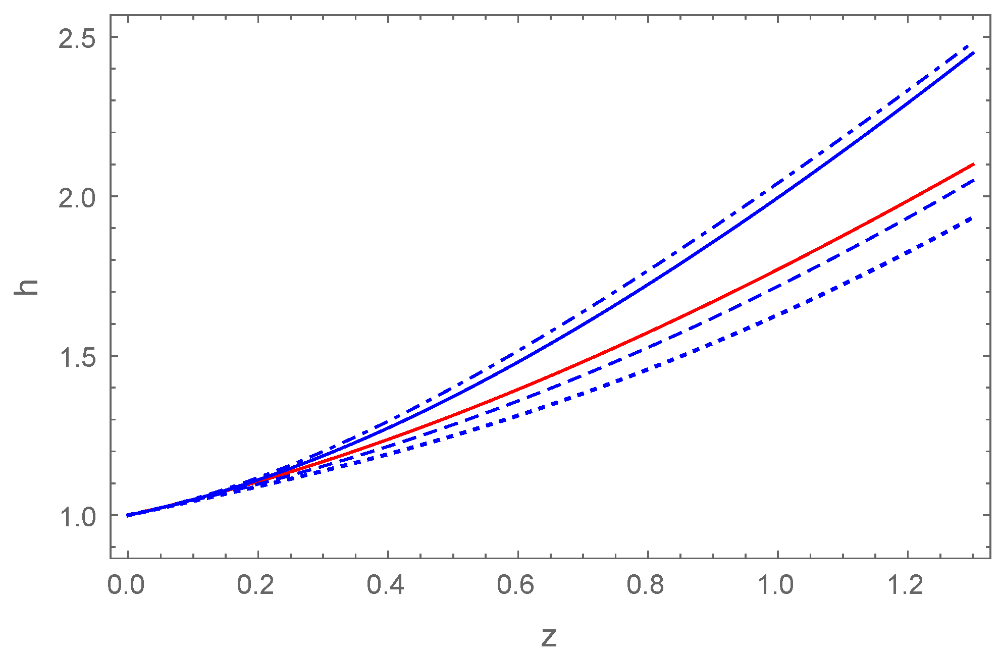
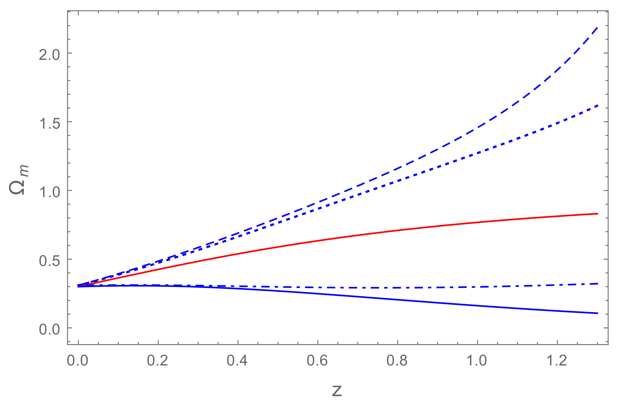
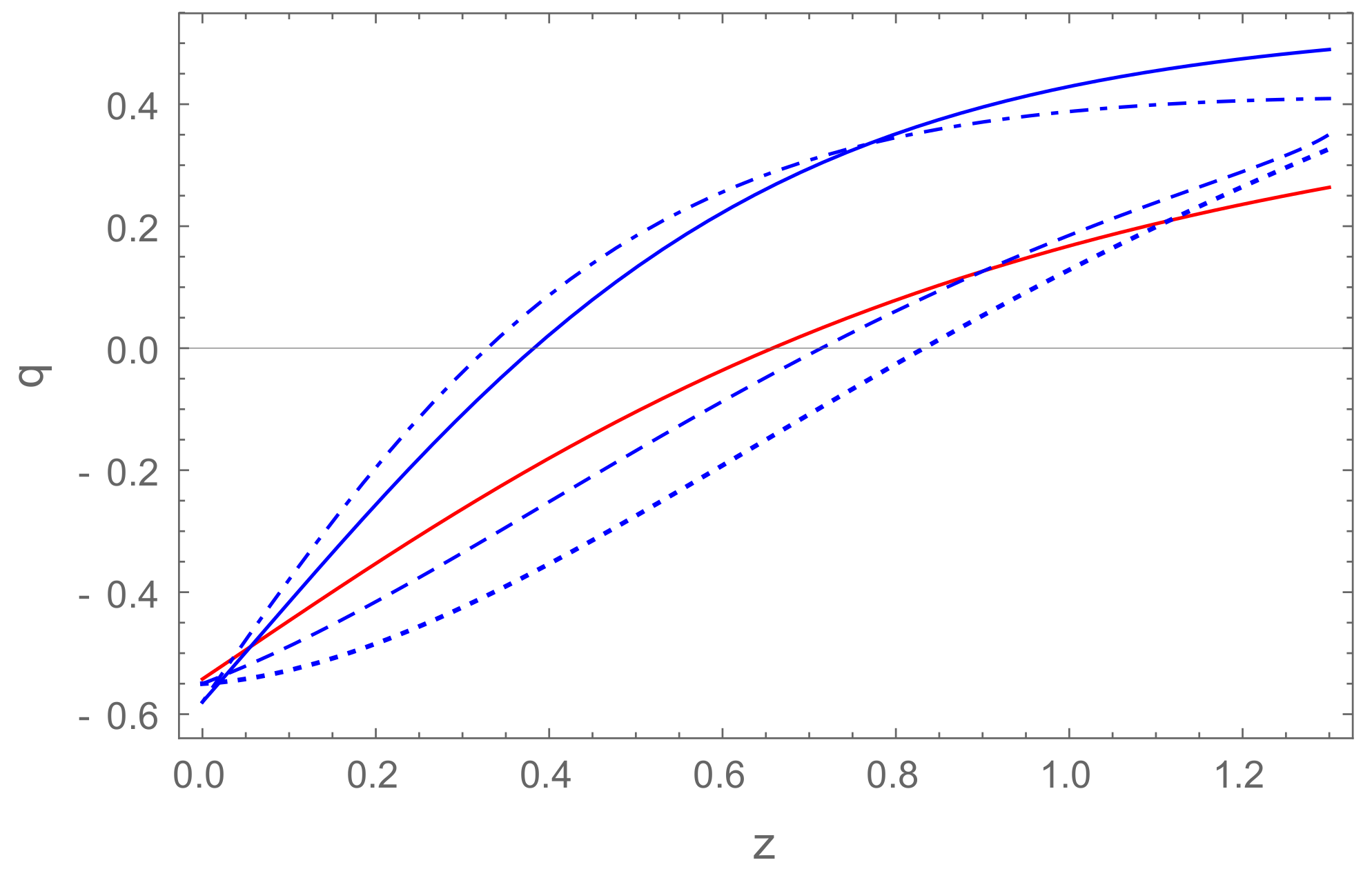
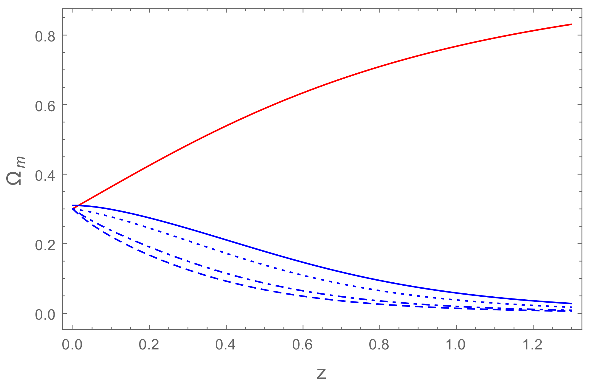
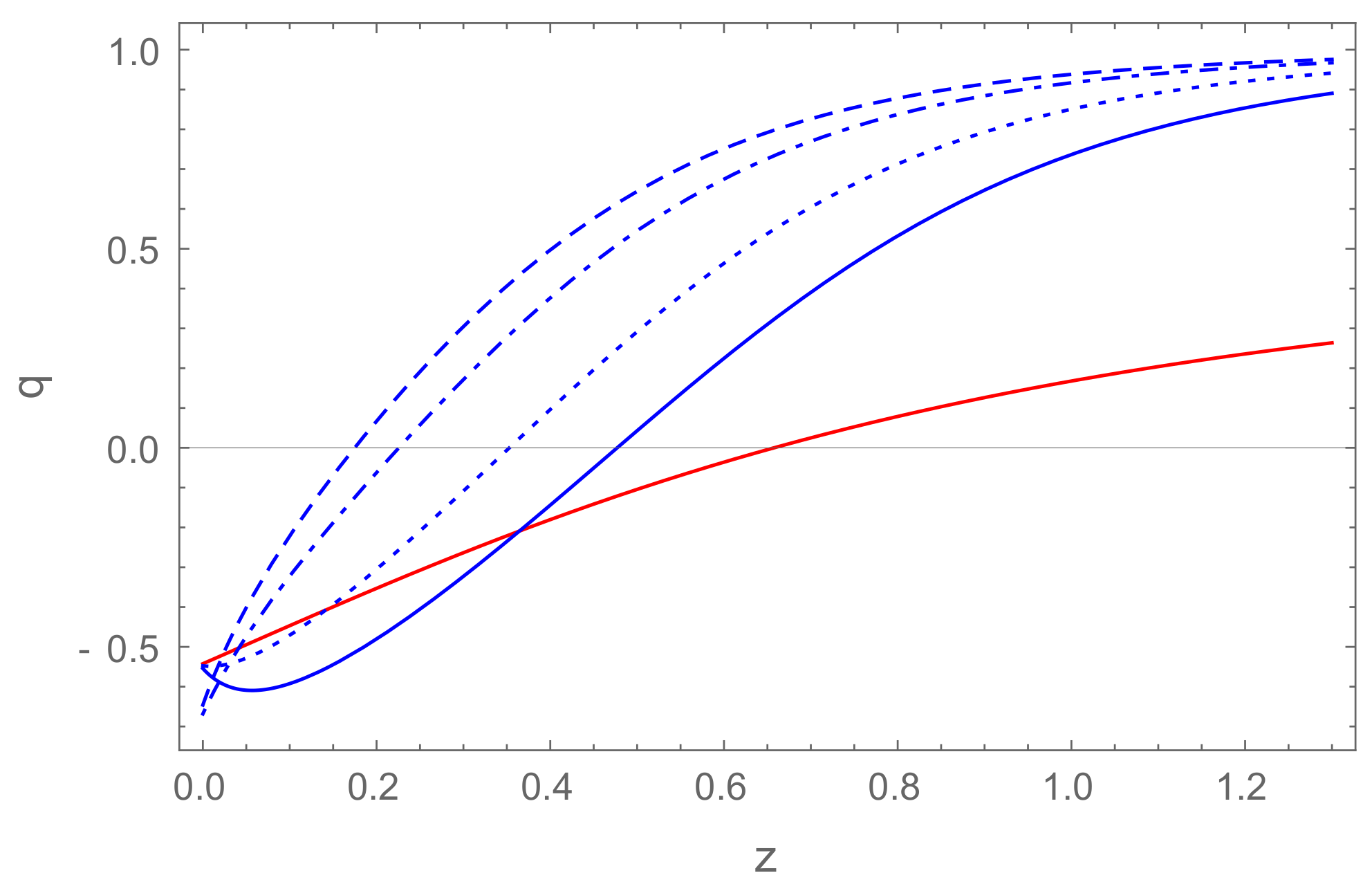
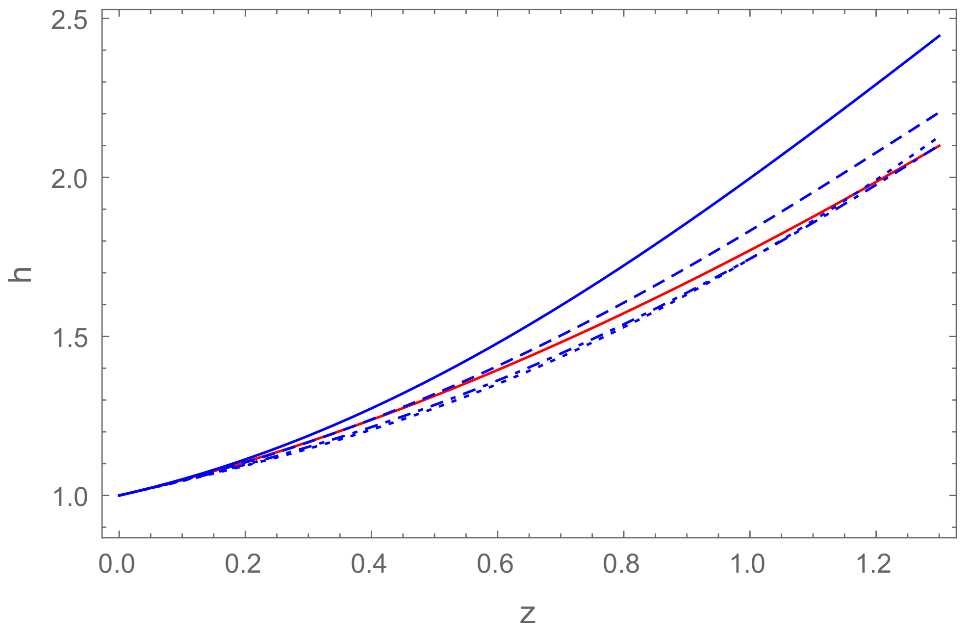
Figure 1, Figure 2 and Figure 3 show the cosmological parameters , and , obtained by numerically solving the generalized Friedmann equations, for different values of and . One can see that there are ascending and descending curves for the density parameter, depending on the values of the pair of the parameters . Additionally, an accelerated phase is present at late times, while, for earlier times, a decelerating phase is found.
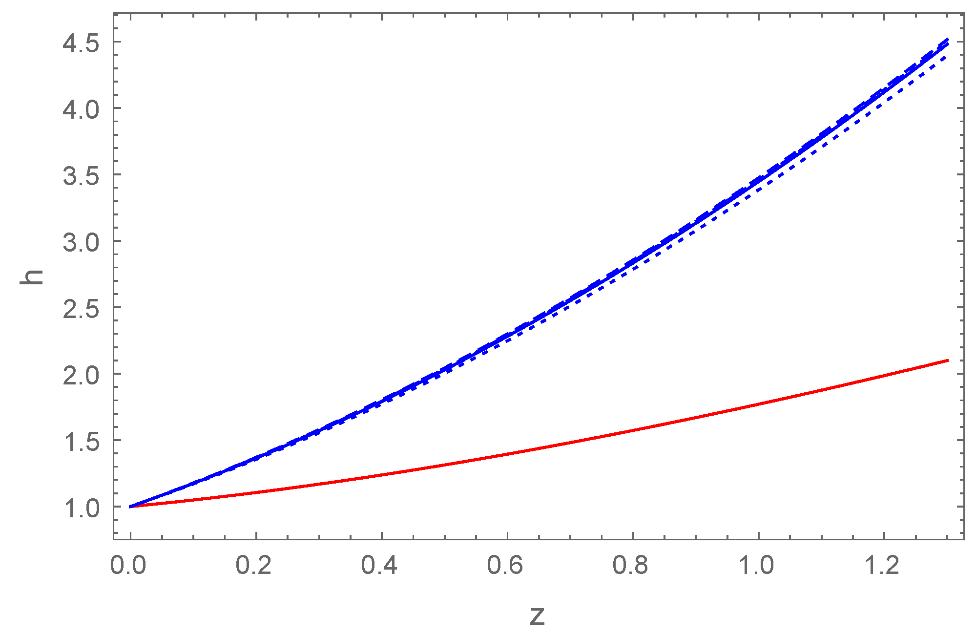
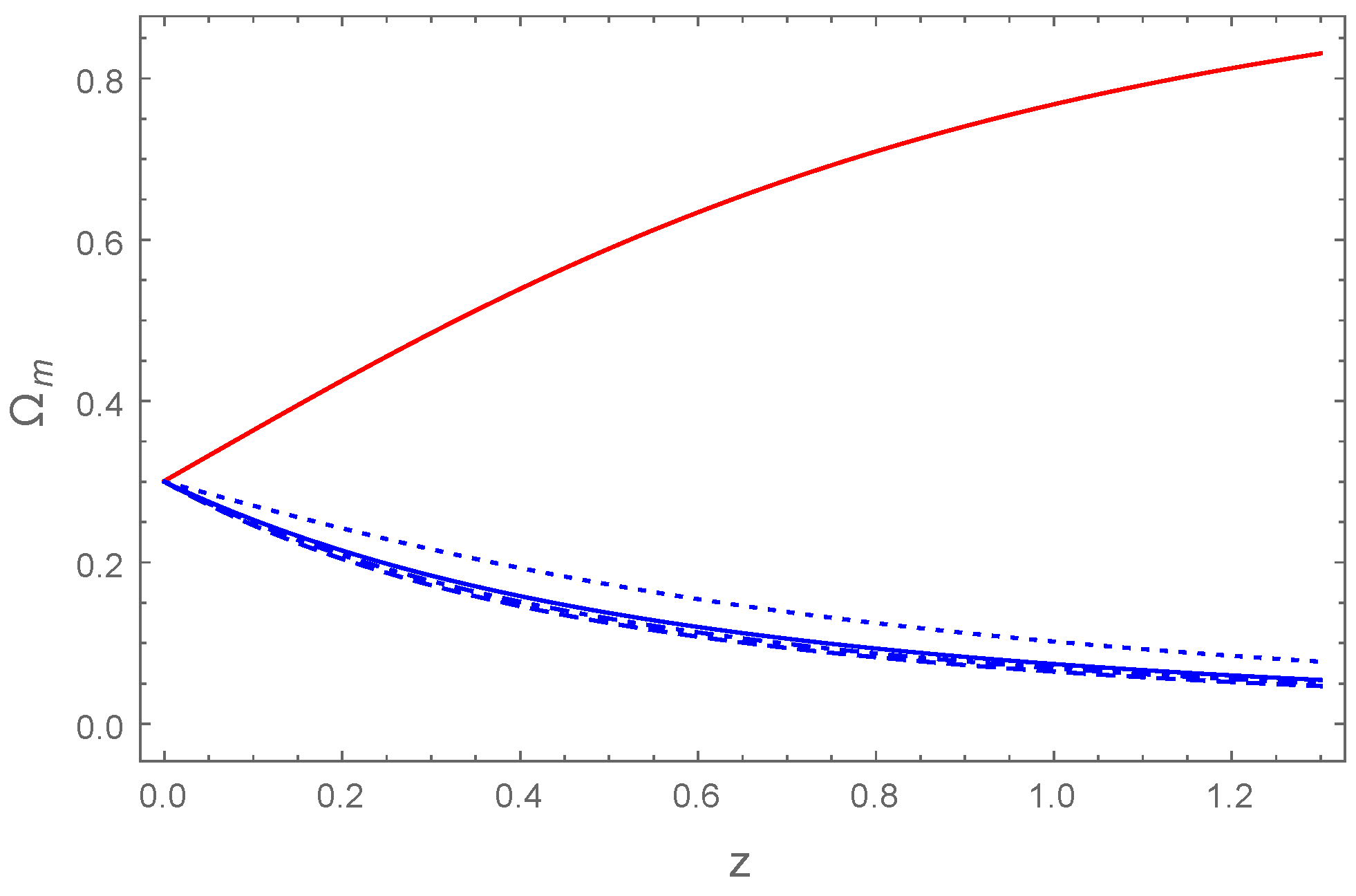
As shown in Figure 1, the Hubble function is an increasing function of the redshift z (and a decreasing function of time), indicating an expansionary evolution of the universe. The evolution of h depends strongly on the model parameters and . For low redshifts , the evolution is basically independent of and . The model can reproduce well the evolution of h in the standard CDM model. The matter density, displayed in Figure 2, shows significant differences with respect to standard cosmology. For the chosen set of parameters, two different behaviors can be observed.
The matter energy density is either increasing or decreasing function of z (decreasing or increasing function of time). The latter case, implying a matter density that increases in time, may be considered unphysical. A scenario with an almost constant density is also possible. For the adopted set of parameters, the evolution of the matter density is significantly different from the evolution of the matter density in the CDM model.
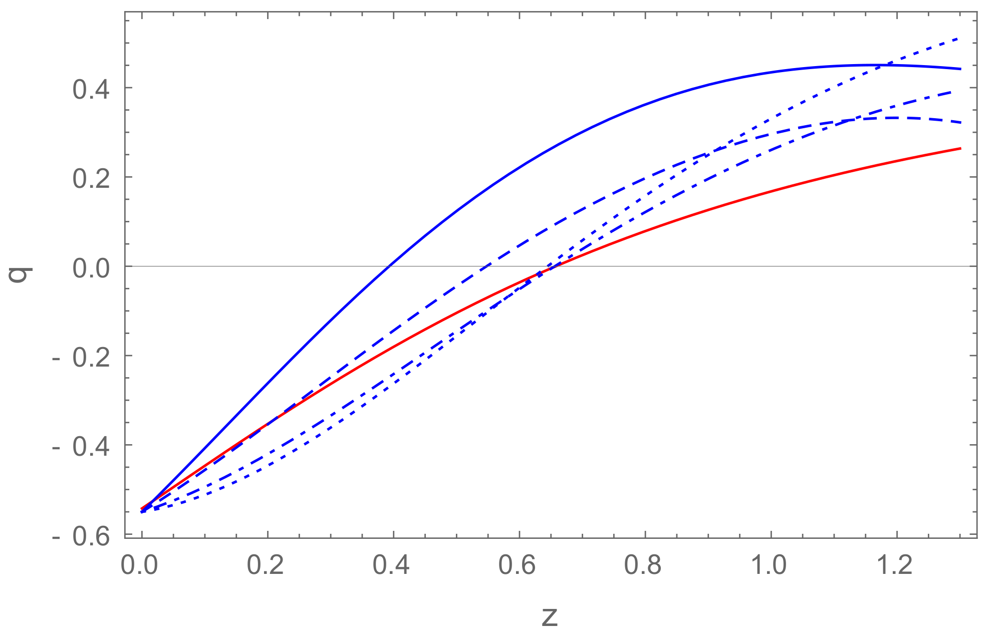
The deceleration parameter, q, shown in Figure 3, indicates the existence of a transition from the decelerating to an accelerating expansion. The evolution of q is strongly dependent on the model parameters, and a wide variety of cosmological behaviors can be constructed. The evolution of q in standard cosmology can also be reproduced.
4.2.
In this Subsection, the expression of the fluctuation tensor , containing only the energy-momentum tensor, is considered. Hence, the term is ignored, since it corresponds to a term proportional to the metric tensor. Therefore, the tensor is given in this case by:
The dimensionless parameters and are defined as:
The non-zero component of Equation (10) is:
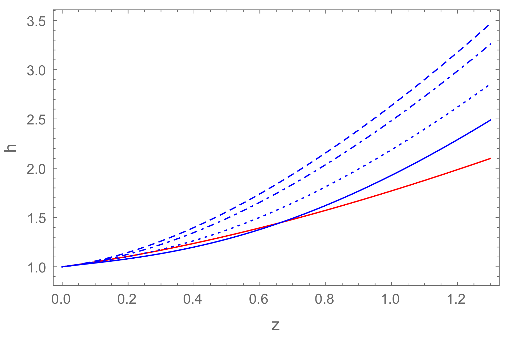
In Figure 4, Figure 5 and Figure 6 the behaviors of the Hubble function, the matter density and the deceleration parameters are shown for different values of the parameters and .
The Hubble function, , represented in Figure 4, is an increasing function of z, and it can reproduce the evolution of the Hubble function in the standard CDM model.
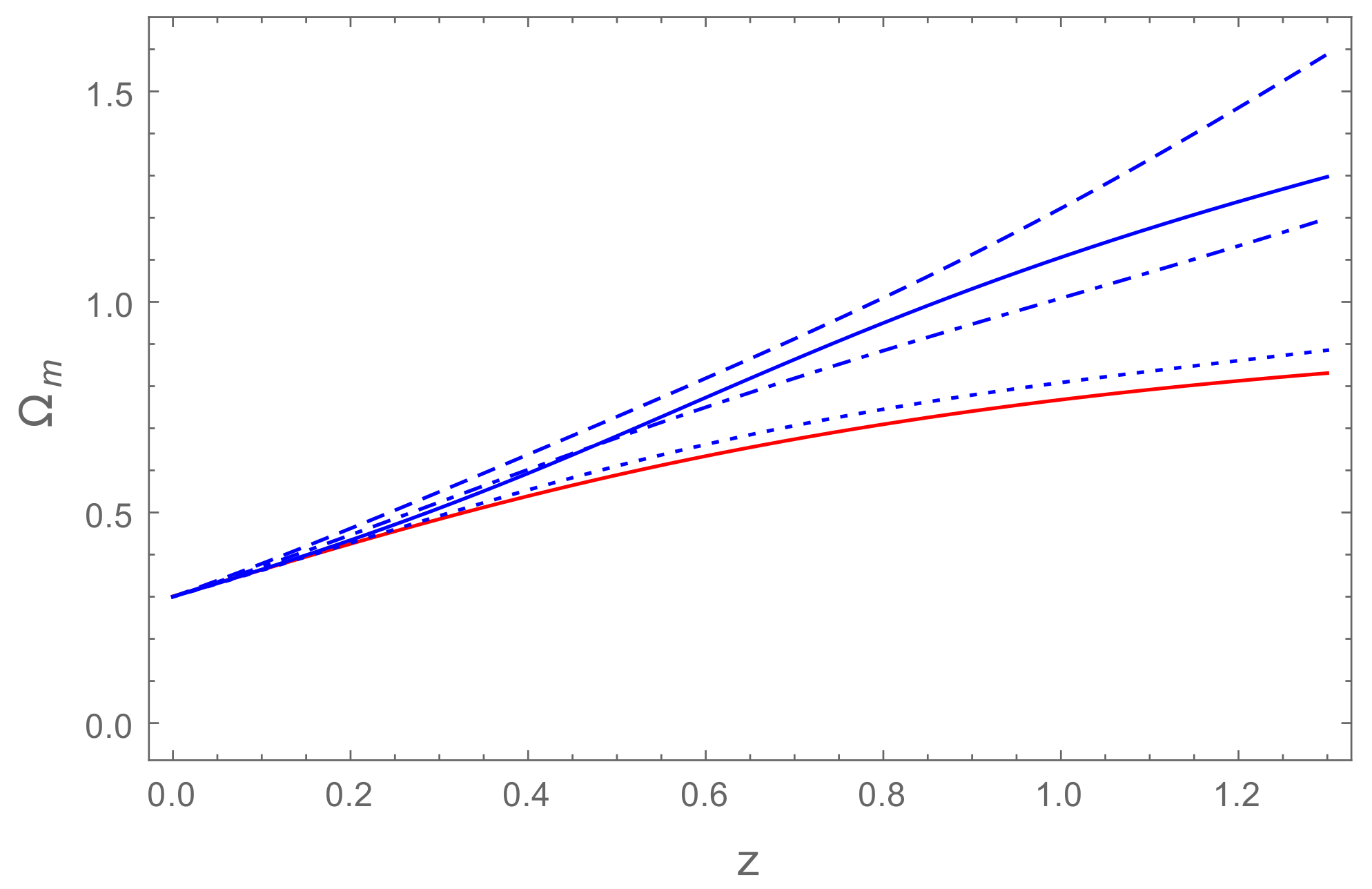
However, significant differences do appear in the behavior of the matter density, as shown in Figure 5. As opposed to the matter behavior in standard cosmology, in this model, the matter energy density is an increasing function of time. Moreover, its the evolution is significantly different compared to the matter density evolution in the standard CDM model for all adopted values of the model parameters.
However, the deceleration parameter q, shown in Figure 6, indicates a transition from a decelerating to an accelerating phase, which can reproduce the present day value of q.
4.3.
Now, let us consider the case where , . Hence, the expression of ,
is obtained.
In this case, the field equations are:
and
and the temporal component of Equation (10) in terms of redshift is:
The evolution in terms of redshift z of the cosmological parameters h, and q are shown in Figure 7, Figure 8 and Figure 9 for different values of the parameters and . In this case, as well as in all other cases the parameters were chosen in such a way to obtain the closest possible approximation of the CDM model.
The Hubble function, h, presented in Figure 7, is an increasing function of z and reproduces well the standard CDM model. For low redshifts, the behavior of h is basically independent on the model parameters.
The ordinary matter density, , shown in Figure 8, is found to be a monotonically decreasing function of time, whose evolution at high redshifts is strongly dependent on the model parameters. For a particular set of values of and , the variation of in the standard cosmological model is reproduced almost exactly.
The deceleration parameter, q, represented in Figure 9, shows a transition from a decelerating to an accelerating cosmological phase. The evolution of the deceleration parameter depends strongly on the adopted numerical values of the model parameters, and . For a range of these parameters, the present model can reproduce quite well the behavior of q at low redshifts.
4.4.
Finally, let us consider the case when only the coefficient is kept in Equation (19), with all the other coefficients set to zero. Hence,
is obtained.
Let us also introduce the dimensionless parameter defined as:
With the use of Equations (A1) and (A2), one can obtain the Friedmann and Raychaudhuri equations in terms of redshift for this case:
The divergence of the energy-momentum tensor (10) takes the form:
The evolutions in terms of redshift z of the Hubble parameter, h, the density parameter, , and the deceleration parameter, q, are shown in Figure 10, Figure 11 and Figure 12. The curves are obtained for different values of the parameter .
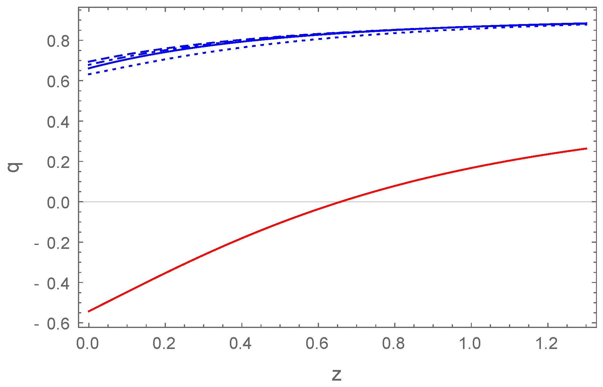
For this choice of , no accelerating expansion at late times is found. The evolution of the universe is still expansionary, as shown by the evolution of the Hubble function in Figure 10. The matter density, shown in Figure 11, is a decreasing function of the redshift, in contrast with the CDM model, indicating an increase of the matter density in time. This effect is due to the non-conservation of the energy-momentum tensor of Equation (51). As one can see from Figure 12, the deceleration parameter is positive, and is roughly constant in the considered range of z. The variation of the numerical values of the parameter has a little effect on the behavior of the cosmological parameters , q and h.
5. Discussions and Final Remarks
The search for quantum gravity is one of the major topics of interest in nowadays theoretical physics. However, despite the intensive effort invested in this direction, the quantum properties of gravity are still elusive, and we presently lack a theory fully unifying the two basic branches of physics. Hence, in order to have at least a basic understanding of the quantum properties of gravity, we need to resort to some mathematical approximations, or to some qualitative approaches. One of such semiclassical directions of research was proposed in [55,57], and it is based on the idea of the decomposition of the quantum metric into two components, one being the classical metric tensor, while the second one is a fluctuating tensor, of quantum origin. By adopting another semiclassical approximation, one can substitute the quantum fluctuating part by the average value of the tensor , representing an effective classical term to be added to the standard metric of general relativity.
A first interesting consequence of this approach is that it leads, in the first order of approximation and on a classical level, to several classes of modified gravity theories, with geometry-matter coupling. For example, by assuming that, a particular class of the modified gravity theory [98] as a function of the Ricchi scalar, R, and the trace of the energy-momentum tensor T, with geometry-matter coupling is obtained. These extensions of standard general relativity have been intensively studied in their different versions [98], but the possible relation with effective semiclassical theories of gravity has not been pointed out. Modified gravity theories with quantum metric fluctuations, even formulated in a semiclassical and effective form may give some insights into the quantum nature of gravity, and its manifestations at the level of the classical world. An important property of all modified theories with geometry-matter coupling is the non-conservation of the matter energy-momentum tensor. This is also a basic property of quantum field theories in curved space-times. Hence, the particle creation processes present in modified gravity theories with geometry-matter coupling may point towards a possible relation between these classes of theories and quantum effects in gravity.
However, in the general formulation of the modified gravity theories in the presence of quantum metric fluctuations, the mathematical form of the fluctuation tensor is arbitrary. In the present paper, the functional form of is fixed by considering the Newtonian limit of the theory. This leads to the derivation of the generalized Poisson equation, which contains several correction terms, with respect to its standard form. By requiring that the model passes the standard tests of gravity at the level of the Solar System, we can fix the form of the fluctuation tensor as given by Equation (19). Generally, can be obtained as a linear combination of the Ricci tensor, the energy-momentum tensor, and the metric tensor, with the coefficients functions of the Ricci scalar R and of the trace of the energy-momentum tensor T.
As a next step, in this investigation, the quantum corrected classical Lagrangian is obtained along with the general effective Einstein equations, corresponding to an arbitrary [61]. Then, using the general form of , a few classes of cosmological models can be constructed that are consistent with the Solar System tests. More exactly, four classes of models are studied. In the first two models, is proportional to the Ricci tensor, and the matter energy-momentum tensor, respectively, with the proportionality coefficients given by linear combinations of R and T. In the third model, we have assumed that can be obtained as a linear combination of the Ricci tensor and the energy-momentum tensor. In the fourth model, is determined by the energy-momentum tensor and its trace only, i.e., by the properties of the matter filling the universe.
A detailed investigation of the cosmological properties of the models, obtained for these specific functional forms of , was performed using numerical methods. Exact solutions of the field equations seem to be impossible to be found, due to the extreme mathematical complexity of the generalized Friedmann equations. The behavior of the Hubble function, of the matter density and of the deceleration parameter were investigated, and for each case, the model predictions are compared with the cosmological results, obtained in the framework of the standard CDM model. Overall, the cosmological evolution strongly depends on the choice of the function , and of the parameters of the specific models. Generally, the models can reproduce the predictions of the standard CDM model, and, thus, describe both decelerating and accelerating phases. To test these models, a detailed comparison with the observational data is necessary. In the present approach, a phenomenological approach is used, by adopting, for the quantum perturbation tensor, some specific functional forms that passes the Solar System tests. However, even this strong criterion cannot uniquely fix the form of , and, thus, for different choices of the quantum perturbation tensor drastically different astrophysical and cosmological behaviors may emerge.
In most of the considered models, in the large time (small redshift) limit, the universe enters into an accelerating phase. The present day value of the deceleration parameter can be obtained for large range of parameter values for the first three considered forms of . By varying the model parameters, a wide variety of cosmological evolutions can be constructed, with some of them reproducing almost exactly the results of the standard CDM model. However, other models do show significant deviations from it. If the variations of the Hubble function and of the deceleration parameter are, for the first three models, qualitatively consistent with observations, some significant differences do appear in the evolution of the matter density. In the first, the second and the fourth here considered cosmological models, for some specific values of parameters the matter energy-density is increasing in time. This unusual behavior is a direct consequence of the non-conservation of the energy-momentum tensor, which can also be interpreted as related to the creation of ordinary matter by the gravitational field. Such processes may play an important role in the early stages of the evolution of the universe, as possible alternatives to the reheating phase of the post-inflationary era. We would also like to point out is that purely decelerating cosmological evolution over a large range of redshifts can also be obtained.
The ultimate challenge present day theoretical physics faces is the problem of the quantization of the gravitational field. Unfortunately no exact solutions for this problem are known. Hence to answer the question of the existence of quantum effects in gravity one should resort to approximate, semiclassical methods. A promising way in this direction could be represented by the consideration, in an additive way, of some tensor fluctuating terms in the metric. The quantum mechanical origin of these terms can be well motivated physically. Such approaches lead to classical gravity models with geometry-matter coupling, and to the non-conservation of the matter energy-momentum tensor. Consequently, the particle production processes, specific to these classes of theories, may be an indication of their deep relation with effective descriptions of quantum gravity. On the other hand, the investigations of the gravitational models with fluctuating quantum metrics could lead to a better understanding of the physical basis of the modified gravity theories with geometry-matter coupling. In the present paper, we considered some of the cosmological implications of the modified gravity models, induced by the quantum metric fluctuations, and some basic theoretical and mathematical tools were introduced that might be used for further investigations of the quantum mechanical effects in gravity and in the geometry of the spacetime.
Author Contributions
Conceptualization, Z.H. and T.H.; Formal analysis, Z.H. and T.H.; Investigation, Z.H. and T.H.; Software, Z.H.; Writing—original draft, T.H.; Writing—review and editing, Z.H. and T.H. All authors have read and agreed to the published version of the manuscript.
Funding
This research received no external funding.
Acknowledgments
We would like to thank the two anonymous reviewers for their useful comments and suggestions that helped to improve the paper. T.H. would like to thank the Yat Sen School of the Sun Yat-Sen University in Guangzhou, China, for kind hospitality during the preparation of this paper.
Conflicts of Interest
The authors declare no conflict of interest.
Appendix A. The Generalized Friedmann Equations
The generalized Friedmann and Raychaudhuri equations, obtained by adopting for the fluctuation tensor the expression given by Equation (19), can be written as:
and
with
References
- Hilbert, D. Die Grundlagen der Physik. In Nachrichten von der Gesellschaft der Wissenschaften zu Göttingen–Mathematische-Physikalische Klasse; Vandenhoeck & Ruprecht: Göttingen, Germany, 1915; Volume 1915, pp. 395–407. [Google Scholar]
- Einstein, A. Die Feldgleichungen der Gravitation. In A. Königlich Preussische Akademie der Wissenschaften; Vandenhoeck & Ruprecht: Göttingen, Germany, 1915; Volume 25, pp. 844–847. [Google Scholar]
- Einstein, A. Die Grundlage der allgemeinen Relativitätstheorie. Annalen Phys. 1916, 49, 769. [Google Scholar] [CrossRef] [Green Version]
- Turyshev, S.G. Experimental Tests of General Relativity. Ann. Rev. Nucl. Part. Sci. 2008, 58, 207. [Google Scholar] [CrossRef] [Green Version]
- Will, C.M. The Confrontation between General Relativity and Experiment. Living Rev. Rel. 2014, 17, 4. [Google Scholar] [CrossRef] [Green Version]
- Marchi, F.D.; Cascioli, G. Testing General Relativity in the Solar System: Present and future perspectives. arXiv 2019, arXiv:1911.05561. [Google Scholar] [CrossRef] [Green Version]
- Abbott, B.P.; Abbott, R.; Abbott, T.D.; Abernathy, M.R.; Acernese, F.; Ackley, K.; Adams, C.; Adams, T.; Addesso, P.; Adhikari, R.X.; et al. LIGO Scientific and Virgo Collaborations. Observation of Gravitational Waves from a Binary Black Hole Merger. Phys. Rev. Lett. 2016, 116, 061102. [Google Scholar] [CrossRef]
- Akiyama, K.; Alberdi, A.; Alef, W.; Asada, K.; Azulay, R.; Baczko, A.-K.; Ball, D.; Baloković, M.; Barrett, J.; Bintley, D.; et al. Event Horizon Telescope Collaboration, First M87 Event Horizon Telescope Results. I. The Shadow of the Supermassive Black Hole. Astrophys. J. Lett. 2019, 875, L1. [Google Scholar] [CrossRef]
- Bronstein, M. Quantum theory of weak gravitational fields. Phys. Z. Der Sowjetunion 1936, 9, 140, republished as Bronstein, M. Republication of: Quantum theory of weak gravitational fields. Gen. Relativ. Gravit. 2012, 44, 267. [Google Scholar] [CrossRef]
- Mukhanov, V.; Winitzki, S. Introduction to Quantum Effects in Gravity; Cambridge University Press: Cambridge, UK, 2007. [Google Scholar]
- Kiefer, C. Quantum Gravity, 3rd ed.; Oxford University Press: Oxford, UK, 2012. [Google Scholar]
- Utiyama, R. Invariant Theoretical Interpretation of Interaction. Phys. Rev. 1956, 101, 1597. [Google Scholar] [CrossRef]
- Kibble, T.W.B. Lorentz invariance and the gravitational field. J. Math. Phys. 1961, 2, 212. [Google Scholar] [CrossRef] [Green Version]
- Moller, C. Conservation laws and absolute parallelism in general relativity. K. Dan. Vidensk. Selsk. Mat. Fys. Skr. 1961, 1, 1. [Google Scholar]
- Pellegrini, C.; Plebanski, J. Tetrad fields and gravitational fields. K. Dan. Vidensk. Selsk. Mat. Fys. Skr. 1962, 2, 1. [Google Scholar]
- Hayashi, K.; Nakano, T. Extended translation invariance and associated gauge fields. Prog. Theor. Phys. 1967, 38, 491. [Google Scholar] [CrossRef] [Green Version]
- Blagojevic, M. Gravitation and Gauge Symmetries; IOP Publishing: Bristol, UK, 2002. [Google Scholar]
- Ashtekar, A. New Variables for Classical and Quantum Gravity. Phys. Rev. Lett. 1986, 57, 2244. [Google Scholar] [CrossRef] [PubMed]
- Ashtekar, A. New Hamiltonian formulation of general relativity. Phys. Rev. D 1987, 36, 1587. [Google Scholar] [CrossRef] [PubMed]
- Ashtekar, A. Lectures on Non-perturbative Canonical Gravity. Notes Prepared in Collaboration with R.S. Tate; World Scientific: Singapore, 1991. [Google Scholar]
- Funai, S.S.; Sugawara, H. Current Algebra Formulation of Quantum Gravity and Its Application to Cosmology. arXiv 2020, arXiv:2004.02151. [Google Scholar] [CrossRef]
- Jacobson, T. Thermodynamics of Spacetime: The Einstein Equation of State. Phys. Rev. Lett. 1995, 75, 1260. [Google Scholar] [CrossRef] [Green Version]
- Connes, A. Gravity coupled with matter and the foundation of non-commutative geometry. Commun. Math. Phys. 1996, 182, 155. [Google Scholar] [CrossRef] [Green Version]
- Reuter, M. Nonperturbative evolution equation for quantum gravity. Phys. Rev. D 1998, 57, 971. [Google Scholar] [CrossRef] [Green Version]
- Rovelli, C. Loop Quantum Gravity. Living Rev. Rel. 1998, 1, 1. [Google Scholar] [CrossRef] [Green Version]
- Gambin., R.; Pullin, J. Consistent Discretization and Loop Quantum Geometry. Phys. Rev. Lett. 2005, 94, 101302. [Google Scholar] [CrossRef] [PubMed] [Green Version]
- Ashtekar, A. Gravity and the quantum. New J. Phys. 2005, 7, 198. [Google Scholar] [CrossRef] [Green Version]
- Horava, P. Quantum gravity at a Lifshitz point. Phys. Rev. D 2009, 79, 084008. [Google Scholar] [CrossRef] [Green Version]
- Verlinde, E.P. On the Origin of Gravity and the Laws of Newton. JHEP 2011, 29, 1104. [Google Scholar]
- Møller, C. Les théories Relativistes de la Gravitation; Colloques Internationaux CNRS vol 91; Tonnelat, A., Ed.; CNRS: Paris, France, 1962; pp. 1–96. [Google Scholar]
- Rosenfeld, L. On quantization of fields. Nucl. Phys. 1963, 40, 353. [Google Scholar] [CrossRef]
- Davies, P.C.W. Singularity avoidance and quantum conformal anomalies. Phys. Lett. B 1977, 6, 402. [Google Scholar] [CrossRef]
- Fischetti, M.V.; Hartle, J.B.; Hu, B.L. Quantum Effects in the early Universe. I. Influence of Trace Anomalies on Homogeneous, Isotropic, Classical Geometries. Phys. Rev. D 1979, 20, 1757. [Google Scholar] [CrossRef]
- Starobinsky, A.A. A new type of isotropic cosmological models without singularity. Phys. Lett. B 1980, 91, 99. [Google Scholar] [CrossRef]
- Kibble, T.W.B.; Randjbar-Daemi, S. Non-linear coupling of quantum theory and classical gravity. J. Phys. A Math. Gen. 1980, 13, 141. [Google Scholar] [CrossRef]
- Nojiri, S.; Odintsov, S.D. Quantum deSitter cosmology and phantom matter. Phys. Lett. B 2003, 562, 147. [Google Scholar] [CrossRef] [Green Version]
- Nojiri, S.; Odintsov, S.D. Quantum escape of sudden future singularity. Phys. Lett. B 2004, 595, 1. [Google Scholar]
- Carlip, S. Is Quantum Gravity Necessary? Class. Quant. Grav. 2008, 25, 154010. [Google Scholar] [CrossRef] [Green Version]
- Ho, P.-M.; Kawai, H.; Matsuo, Y.; Yokokura, Y. Back reaction of 4D conformal fields on static black-hole geometry. JHEP 2018, 56, 11. [Google Scholar] [CrossRef] [Green Version]
- Han, M. Einstein equation from covariant loop quantum gravity in semiclassical continuum limit. Phys. Rev. D 2017, 96, 024047. [Google Scholar] [CrossRef] [Green Version]
- dos Reis, E.A.; Krein, G.; de Paula Netto, T.; Shapiro, I.L. Stochastic quantization of a self-interacting nonminimal scalar field in semiclassical gravity. Phys. Lett. B 2019, 798, 134925. [Google Scholar] [CrossRef]
- Juárez-Aubry, A. Semi-classical gravity in de Sitter spacetime and the cosmological constant. Phys. Lett. B 2019, 797, 134912. [Google Scholar] [CrossRef]
- Satin, S. Correspondences of matter fluctuations in semiclassical and classical gravity for cosmological spacetime. Phys. Rev. D 2019, 100, 044032. [Google Scholar] [CrossRef] [Green Version]
- Matsui, H.; Watamura, N. Quantum spacetime instability and breakdown of semiclassical gravity. Phys. Rev. D 2020, 101, 025014. [Google Scholar] [CrossRef] [Green Version]
- Parisi, G.; Wu, Y.S. Perturbation Theory Without Gauge Fixing. Sci. Sin. 1981, 24, 483. [Google Scholar]
- Nelson, E. Derivation of the Schrödinger Equation from Newtonian Mechanics. Phys. Rev. 1966, 150, 1079. [Google Scholar] [CrossRef]
- Damgaard, P.H.; Huffel, H. Stochastic Quantization; World Scientific: Singapore, 1988. [Google Scholar]
- Namiki, M. Basic Ideas of Stochastic Quantization. Prog. Theor. Phys. Suppl. 1993, 1, 111. [Google Scholar] [CrossRef] [Green Version]
- Rumpf, H. Stochastic quantization of Einstein gravity. Phys. Rev. D 1986, 942, 33. [Google Scholar] [CrossRef]
- Rumpf, H. Stochastic Quantum Gravity in D Dimension. Prog. Theor. Phys. Suppl. 1993, 111, 63. [Google Scholar] [CrossRef] [Green Version]
- Hu, B.L.; Roura, A.; Verdaguer, E. Induced quantum metric fluctuations and the validity of semiclassical gravity. Phys. Rev. D 2004, 70, 044002. [Google Scholar] [CrossRef] [Green Version]
- Satin, S.; Cho, H.T.; Hu, B.L. Conformally-related Einstein-Langevin equations for metric fluctuations in stochastic gravity. Phys. Rev. D 2016, 94, 064019. [Google Scholar] [CrossRef] [Green Version]
- Wheeler, J.A. On the nature of quantum geometrodynamics. Ann. Phys. 1957, 2, 604. [Google Scholar] [CrossRef]
- Misner, C.W.; Thorne, K.S.; Wheeler, J.A. Gravitation; W. H. Freeman: San Francisco, CA, USA, 1973. [Google Scholar]
- Dzhunushaliev, V.; Folomeev, V.; Kleihaus, B.; Kunz, J. Modified gravity from the quantum part of the metric. Eur. Phys. J. C 2014, 74, 2743. [Google Scholar] [CrossRef] [Green Version]
- Dzhunushaliev, V.; Folomeev, V.; Kleihaus, B.; Kunz, J. Modified gravity from the nonperturbative quantization of a metric. Eur. Phys. J. C 2015, 75, 157. [Google Scholar] [CrossRef] [PubMed] [Green Version]
- Yang, R.-J. Effects of quantum fluctuations of metric on the universe. Phys. Dark Univ. 2016, 13, 87. [Google Scholar] [CrossRef] [Green Version]
- Dzhunushaliev, V. Nonperturbative quantization: Ideas, perspectives, and applications. arXiv 2015, arXiv:1505.02747. [Google Scholar]
- Dzhunushaliev, V.; Quevedo, H. Einstein equations with fluctuating volume. Gravit. Cosmol. 2017, 23, 280. [Google Scholar] [CrossRef] [Green Version]
- Dzhunushaliev, V.; Folomeev, V.; Quevedo, H. Nonperturbative Quantization à La Heisenberg: Modified Gravities, Wheeler-DeWitt Equations, and Monopoles in QCD. Gravit. Cosmol. 2019, 25, 1. [Google Scholar] [CrossRef]
- Liu, X.; Harko, T.; Liang, S.-D. Cosmological implications of modified gravity induced by quantum metric fluctuations. Eur. Phys. J. C 2016, 76, 420. [Google Scholar] [CrossRef] [Green Version]
- Perlmutter, S.; Aldering, G.; Goldhaber, G.; Knop, R.A.; Nugent, P.; Castro, P.G.; Deustua, S.; Fabbro, S.; Goobar, A.; Groom, D.E.; et al. Measurements of Ω and Λ from 42 High-Redshift Supernovae. Astrophys. J. 1999, 517, 565. [Google Scholar] [CrossRef]
- Knop, R.A.; Aldering, G.; Amanullah, R.; Astier, P.; Blanc, G.; Burns, M.S.; Conley, A.; Deustua, S.E.; Doi, M.; Ellis, R.; et al. New Constraints on Ωm, ωΛ, and w from an Independent Set of Eleven High-Redshift Supernovae Observed with HST. Astrophys. J. 2003, 598, 102. [Google Scholar] [CrossRef] [Green Version]
- Riess, A.G.; Strolger, L.-G.; Casertano, S.; Ferguson, H.C.; Mobasher, B.; Gold, B.; Challis, P.J.; Filippenko, A.V.; Jha, S.; Li, W.; et al. New Hubble Space Telescope Discoveries of Type Ia Supernovae at z > 1: Narrowing Constraints on the Early Behavior of Dark Energy. Astrophys. J. 2007, 659, 98. [Google Scholar] [CrossRef] [Green Version]
- Amanullah, R.; Lidman, C.; Rubin, D.; Aldering, G.; Astier, P.; Barbary, K.; Burns, M.S.; Conley, A.; Dawson, K.S.; Deustua, S.E.; et al. Spectra and Light Curves of Six Type Ia Supernovae at 0.511<z < 1.12 and the Union2 Compilation. Astrophys. J. 2010, 716, 712. [Google Scholar] [CrossRef] [Green Version]
- Weinberg, D.H.; Mortonson, M.J.; Eisenstein, D.J.; Hirata, C.; Riess, A.G.; Rozo, E. Observational probes of cosmic acceleration. Phys. Rep. 2013, 530, 87. [Google Scholar] [CrossRef] [Green Version]
- Aad, G.; Abbott, B.; Abdallah, J.; Abdinov, O.; Aben, R.; Abolins, M.; Abouzeid, O.S.; Abramowicz, H.; Abreu, H.; Abreu, R.; et al. Search for Dark Matter in Events with Missing Transverse Momentum and a Higgs Boson Decaying to Two Photons in pp Collisions at s=8 TeV with the ATLAS Detector. Phys. Rev. Lett. 2015, 115, 131801. [Google Scholar] [CrossRef] [Green Version]
- Peebles, P.J.E.; Ratra, B. The cosmological constant and dark energy. Rev. Mod. Phys. 2003, 75, 559. [Google Scholar] [CrossRef] [Green Version]
- Padmanabhan, T. Cosmological Constant—The Weight of the Vacuum. Phys. Repts. 2003, 380, 235. [Google Scholar] [CrossRef] [Green Version]
- Overduin, J.M.; Wesson, P.S. Dark Matter and Background Light. Phys. Rep. 2004, 402, 267. [Google Scholar] [CrossRef] [Green Version]
- Baer, H.; Choi, K.-Y.; Kim, J.E.; Roszkowski, L. Dark matter production in the early Universe: Beyond the thermal WIMP paradigm. Phys. Rep. 2015, 555, 1. [Google Scholar] [CrossRef] [Green Version]
- Weinberg, S. The cosmological constant problem. Rev. Mod. Phys. 1989, 61, 1. [Google Scholar] [CrossRef]
- Weinberg, S. The Cosmological Constant Problems (Talk given at Dark Matter 2000, February, 2000). arXiv 2000, arXiv:astro-ph/0005265. [Google Scholar]
- Buchdahl, H.A. Non-Linear Lagrangians and Cosmological Theory. Mon. Not. Roy. Astron. Soc. 1970, 150, 1. [Google Scholar] [CrossRef] [Green Version]
- Silvestri, A.; Trodden, M. Approaches to Understanding Cosmic Acceleration. Rept. Prog. Phys. 2009, 72, 096901. [Google Scholar] [CrossRef] [Green Version]
- De Felice, A.; Tsujikawa, S. f(R) theories. Living Rev. Rel. 2010, 13, 3. [Google Scholar] [CrossRef] [PubMed] [Green Version]
- Sotiriou, T.P.; Faraoni, V. f(R) theories of gravity. Rev. Mod. Phys. 2010, 82, 451. [Google Scholar] [CrossRef] [Green Version]
- Capozziello, S.; De Laurentis, M. Extended Theories of Gravity. Phys. Rept. 2011, 509, 167. [Google Scholar] [CrossRef] [Green Version]
- Nojiri, S.; Odintsov, S.D. Unified cosmic history in modified gravity: From F(R) theory to Lorentz non-invariant models. Phys. Rept. 2011, 505, 59. [Google Scholar] [CrossRef] [Green Version]
- Haghani, Z.; Harko, T.; Sepangi, H.R.; Shahidi, S. Matter may matter. Int. J. Mod. Phys. D 2014, 23, 1442016. [Google Scholar] [CrossRef] [Green Version]
- Bertolami, O.; Boehmer, C.G.; Harko, T.; Lobo, F.S.N. Extra force in f(R) modified theories of gravity. Phys. Rev. D 2007, 75, 104016. [Google Scholar] [CrossRef] [Green Version]
- Harko, T. Modified gravity with arbitrary coupling between matter and geometry. Phys. Lett. B 2008, 669, 376. [Google Scholar] [CrossRef] [Green Version]
- Harko, T.; Lobo, F.S.N. f(R,Lm) gravity. Eur. Phys. J. C 2010, 70, 373. [Google Scholar] [CrossRef]
- Harko, T.; Lobo, F.S.N.; Minazzoli, O. Extended f(R,Lm) gravity with generalized scalar field and kinetic term dependences. Phys. Rev. D 2013, 87, 047501. [Google Scholar] [CrossRef] [Green Version]
- Harko, T.; Lobo, F.S.N.; Nojiri, S.; Odintsov, S.D. f(R, T) gravity. Phys. Rev. D 2011, 84, 024020. [Google Scholar] [CrossRef] [Green Version]
- Harko, T. Thermodynamic interpretation of the generalized gravity models with geometry-matter coupling. Phys. Rev. D 2014, 90, 044067. [Google Scholar] [CrossRef] [Green Version]
- Haghani, Z.; Harko, T.; Lobo, F.S.N.; Sepangi, H.R.; Shahidi, S. Further matters in space-time geometry: f(R,T,RμνTμν) gravity. Phys. Rev. D 2013, 88, 044023. [Google Scholar] [CrossRef] [Green Version]
- Odintsov, S.D.; Sáez-Gómez, D. f(R,T,RμνTμν) gravity phenomenology and ΛCDM universe. Phys. Lett. B 2013, 725, 437. [Google Scholar] [CrossRef]
- Harko, T.; Koivisto, T.S.; Lobo, F.S.N.; Olmo, G.J. Metric-Palatini gravity unifying local constraints and late-time cosmic acceleration. Phys. Rev. D 2012, 85, 084016. [Google Scholar] [CrossRef] [Green Version]
- Tamanini, N.; Böhmer, C.G. Generalized hybrid metric-Palatini gravity. Phys. Rev. D 2013, 87, 084031. [Google Scholar] [CrossRef] [Green Version]
- Capozziello, S.; Harko, T.; Koivisto, T.S.; Lobo, F.S.N.; Olmo, G.J. Hybrid metric-Palatini gravity. Universe 2015, 1, 199. [Google Scholar] [CrossRef]
- Haghani, Z.; Harko, T.; Sepangi, H.R.; Shahidi, S. Weyl-Cartan-Weitzenböck gravity as a generalization of teleparallel gravity. JCAP 2012, 10, 061. [Google Scholar] [CrossRef] [Green Version]
- Harko, T.; Koivisto, T.S.; Lobo, F.S.N.; Olmo, G.J.; Rubiera-Garcia, D. Coupling matter in modified Q gravity. Phys. Rev. D 2018, 98, 084043. [Google Scholar] [CrossRef] [Green Version]
- Xu, Y.; Li, G.; Harko, T.; Liang, S.-D. f(Q, T) gravity. Eur. Phys. J. C 2019, 79, 708. [Google Scholar] [CrossRef] [Green Version]
- Harko, T.; Lobo, F.S.N.; Otalora, G.; Saridakis, E.N. f(T,) gravity and cosmology. JCAP 2014, 21, 12. [Google Scholar] [CrossRef] [Green Version]
- Harko, T.; Lobo, F.S.N.; Saridakis, E.N. Cosmology with higher-derivative matter fields. Int. J. Geom. Meth. Mod. Phys. 2016, 13, 1650102. [Google Scholar] [CrossRef] [Green Version]
- Harko, T.; Lobo, F.S.N. Generalized Curvature-Matter Couplings in Modified Gravity. Galaxies 2014, 2, 410. [Google Scholar] [CrossRef] [Green Version]
- Harko, T.; Lobo, F.S.N. Extensions of f(R) Gravity: Curvature-Matter Couplings and Hybrid Metric-Palatini Theory; Cambridge University Press: Cambridge, UK, 2018. [Google Scholar]
- Harko, T.; Lobo, F.S.N. Irreversible thermodynamic description of interacting dark energy—Dark matter cosmological models. Phys. Rev. D 2013, 87, 044018. [Google Scholar] [CrossRef] [Green Version]
- Harko, T.; Lobo, F.S.N.; Mimoso, J.P.; Pavón, D. Gravitational induced particle production through a nonminimal curvature-matter coupling. Eur. Phys. J. C 2015, 75, 386. [Google Scholar] [CrossRef] [Green Version]
- Parker, L. Particle Creation in Expanding Universes. Phys. Rev. Lett. 1968, 21, 562. [Google Scholar] [CrossRef]
- Zeldovich, Y.B. Particle Production in Cosmology. J. Exper. Theor. Phys. Lett. 1970, 12, 307. [Google Scholar]
- Parker, L. Quantized Fields and Particle Creation in Expanding Universes. II. Phys. Rev. D 1971, 3, 2546. [Google Scholar] [CrossRef]
- Fulling, S.A. Aspects of Quantum Field Theory in Curved Space-Time; Cambridge University Press: Cambridge, UK, 1989. [Google Scholar]
- Parker, L.E.; Toms, D.J. Quantum Field Theory in Curved Spacetime-Quantized Fields and Gravity; Cambridge University Press: Cambridge, UK, 2009. [Google Scholar]
- Lee, J.-W. Are galaxies extending? Phys. Lett. B 2009, 681, 118. [Google Scholar] [CrossRef] [Green Version]
- Park, C.-G.; Hwang, J.-C.; Noh, H. Axion as a cold dark matter candidate: Low-mass case. Phys. Rev. D 2012, 86, 083535. [Google Scholar] [CrossRef] [Green Version]
- Boucher, W.; Traschen, J. Semiclassical physics and quantum fluctuations. Phys. Rev. D 1988, 37, 3522. [Google Scholar] [CrossRef]
- Capozziello, S.; De Laurentis, M.; De Martino, I.; Formisano, M.; Odintsov, S.D. Jeans analysis of self-gravitating systems in f(R) gravity. Phys. Rev. D 2012, 85, 044022. [Google Scholar] [CrossRef] [Green Version]
- Landau, L.D.; Lifshitz, E.M. The Classical Theory of Fields; Butterworth-Heinemann: Oxford, UK, 1998. [Google Scholar]
- Riess, A.G.; Filippenko, A.V.; Challis, P.; Clocchiatti, A.; Diercks, A.; Garnavich, P.M.; Gilliland, R.L.; Hogan, C.J.; Jha, S.; Kirshner, R.P.; et al. Observational Evidence from Supernovae for an Accelerating Universe and a Cosmological Constant. Astron. J. 1998, 116, 1009. [Google Scholar] [CrossRef] [Green Version]
- de Bernardis, P.; Ade, P.A.R.; Bock, J.J.; Bond, J.R.; Borrill, J.; Boscaleri, A.; Coble, K.; Crill, B.P.; De Gasperis, G.; Farese, P.C.; et al. A Flat Universe from High-Resolution Maps of the Cosmic Microwave Background Radiation. Nature 2000, 404, 955. [Google Scholar] [CrossRef]
- Hanany, S.; Ade, P.; Balbi, A.; Bock, J.; Borrill, J.; Boscaleri, A.; de Bernardis, P.; Ferreira, P.G.; Hristov, V.V.; Jaffe, A.H.; et al. MAXIMA-1: A Measurement of the Cosmic Microwave Background Anisotropy on angular scales of 10 arcminutes to 5 degrees. Astrophys. J. 2000, 545, L5. [Google Scholar] [CrossRef]
- Riess, A.G.; Macri, L.; Casertano, S.; Lampeitl, H.; Ferguson, H.C.; Filippenko, A.V.; Jha, S.W.; Li, W.; Chornock, R.A. 3% Solution: Determination of the Hubble Constant with the Hubble space Telescopr and Wide Field Camera 3. Astrophys. J. 2011, 730, 119. [Google Scholar] [CrossRef] [Green Version]
- Ade, P.A.R.; Aghanim, N.; Arnaud, M.; Ashdown, M.; Aumont, J.; Baccigalupi, C.; Banday, A.J.; Barreiro, R.B.; Bartlett, J.G.; Bartolo, N.; et al. Planck collaboration, Planck 2015 results. XIII. Cosmological parameters. Astron. Astrophys. 2016, 594, A13. [Google Scholar] [CrossRef] [Green Version]
- Aghanim, N.; Akrami, Y.; Arroja, F.; Ashdown, M.; Aumont, J.; Baccigalupi, C.; Ballardini, M.; Banday, A.J.; Barreiro, R.B.; Bartolo, N.; et al. Planck 2018 results. I. Overview and the cosmological legacy of Planck. Astron. Astrophys. 2020, 641, A1. [Google Scholar] [CrossRef] [Green Version]
- Aghanim, N.; Akrami, Y.; Ashdown, M.; Aumont, J.; Baccigalupi, C.; Ballardini, M.; Banday, A.J.; Barreiro, R.B.; Bartolo, N.; Basak, S.; et al. Planck 2018 results. VI. Cosmological parameters. Astron. Astrophys. 2020, 641, A6. [Google Scholar] [CrossRef] [Green Version]
Figure 1.
Variation of the dimensionless Hubble function, h, as a function of the redshift z for the tensor with different values of the parameters and : and (solid curve), and (dotted curve), and (dashed curve), and and (dot-dashed curve). The evolution of the Hubble function in the standard CDM model is represented by the red solid curve.

Figure 2.
Variation of the dimensionless matter density, , as a function of z for with different values of the parameters and : and (solid curve), and (dotted curve), and (dashed curve), and and (dot-dashed curve). The evolution of the matter density in the standard CDM model is shown by the red solid curve.

Figure 3.
Variation of the deceleration parameter, q, as a function of z for with different values of the parameters and : and (solid curve), and (dotted curve), and (dashed curve), and and (dot-dashed curve) The evolution of the deceleration parameter in the standard CDM model is depicted by the red solid curve.

Figure 4.
Variation of the dimensionless Hubble function h as a function of z for with different values of the parameters and : and (solid curve), and (dotted curve), and (dashed curve), and and (dot-dashed curve). The evolution of the Hubble function in the standard CDM model is described by the red solid curve.

Figure 5.
Variation of the dimensionless matter density, , as a function of z for with different values of the parameters and : and (solid curve), and (dotted curve), and (dashed curve), and and (dot-dashed curve). The evolution of the matter density in the standard CDM model corresponds to the red solid curve.

Figure 6.
Variation of the deceleration parameter, q, as a function of z for with different values of the parameters and : and (solid curve), and (dotted curve), and (dashed curve), and and (dot-dashed curve). The evolution of the deceleration parameter in the standard CDM model is described by the red solid curve.

Figure 7.
Variation of the Hubble function h as a function of z for with different values of the parameters and : and (solid curve), and (dotted curve), and (dashed curve), and and (dot-dashed curve). The evolution of the Hubble function in the standard CDM model is described by the red solid curve.

Figure 8.
Variation of the matter density as a function of z for with different values of the parameters and : and (solid curve), and (dotted curve), and (dashed curve), and and (dot-dashed curve). The evolution of the matter density in the standard CDM model is described by the red solid curve.
Figure 8.
Variation of the matter density as a function of z for with different values of the parameters and : and (solid curve), and (dotted curve), and (dashed curve), and and (dot-dashed curve). The evolution of the matter density in the standard CDM model is described by the red solid curve.

Figure 9.
Variation of the deceleration parameter, q, as a function of z for with different values of the parameters and : and (solid curve), and (dotted curve), and (dashed curve), and and (dot-dashed curve). The evolution of the deceleration parameter in the standard CDM model is represented by the red solid curve.

Figure 10.
Variation of the Hubble function, h, as a function of z for with different values of the parameter : (solid curve), (dotted curve), (dashed curve), and (dot-dashed curve). The evolution of the Hubble function in the standard CDM model is represented by the red solid curve.
Figure 10.
Variation of the Hubble function, h, as a function of z for with different values of the parameter : (solid curve), (dotted curve), (dashed curve), and (dot-dashed curve). The evolution of the Hubble function in the standard CDM model is represented by the red solid curve.

Figure 11.
Variation of the matter density, , as a function of z for with different values of the parameter : (solid curve), (dotted curve), (dashed curve), and (dot-dashed curve). The evolution of the matter density in the standard CDM model is represented by the red solid curve.
Figure 11.
Variation of the matter density, , as a function of z for with different values of the parameter : (solid curve), (dotted curve), (dashed curve), and (dot-dashed curve). The evolution of the matter density in the standard CDM model is represented by the red solid curve.

Figure 12.
Variation of the deceleration parameter, q, as a function of z for with different values of the parameter : (solid curve), (dotted curve), (dashed curve), and (dot-dashed curve). The evolution of the deceleration parameter in the standard CDM model is represented by the red solid curve.
Figure 12.
Variation of the deceleration parameter, q, as a function of z for with different values of the parameter : (solid curve), (dotted curve), (dashed curve), and (dot-dashed curve). The evolution of the deceleration parameter in the standard CDM model is represented by the red solid curve.

Publisher’s Note: MDPI stays neutral with regard to jurisdictional claims in published maps and institutional affiliations. |
© 2021 by the authors. Licensee MDPI, Basel, Switzerland. This article is an open access article distributed under the terms and conditions of the Creative Commons Attribution (CC BY) license (https://creativecommons.org/licenses/by/4.0/).
Share and Cite
MDPI and ACS Style
Haghani, Z.; Harko, T. Effects of Quantum Metric Fluctuations on the Cosmological Evolution in Friedmann-Lemaitre-Robertson-Walker Geometries. Physics 2021, 3, 689-714. https://0-doi-org.brum.beds.ac.uk/10.3390/physics3030042
AMA Style
Haghani Z, Harko T. Effects of Quantum Metric Fluctuations on the Cosmological Evolution in Friedmann-Lemaitre-Robertson-Walker Geometries. Physics. 2021; 3(3):689-714. https://0-doi-org.brum.beds.ac.uk/10.3390/physics3030042
Chicago/Turabian StyleHaghani, Zahra, and Tiberiu Harko. 2021. "Effects of Quantum Metric Fluctuations on the Cosmological Evolution in Friedmann-Lemaitre-Robertson-Walker Geometries" Physics 3, no. 3: 689-714. https://0-doi-org.brum.beds.ac.uk/10.3390/physics3030042