Classical Chaos Described by a Density Matrix

Abstract

In this paper, a reference to the semiclassical model, in which quantum degrees of freedom interact with classical ones, is considered. The classical limit of a maximum-entropy density matrix that describes the temporal evolution of such a system is analyzed. Here, it is analytically shown that, in the classical limit, it is possible to reproduce classical results. An example is classical chaos. This is done by means a pure-state density matrix, a rather unexpected result. It is shown that this is possible only if the quantum part of the system is in a special class of states.

1. Introduction

The quantum–classical transition is a frontier issue, a rather transcendental physics topic [1,2,3,4,5]. The use of semi-classical systems to describe problems in physics has a long history; see, e.g., [6,7,8,9,10,11,12]. A particularly important case to be highlighted is the one, in which the quantum features of one of the two components of a composite system are negligible in comparison with those of the other. Regarding the first component as a classical one simplifies the description and provides deep insight into the combined system dynamics [13]. This methodology is used for the interaction of matter with a field. In this effort, one looks at these matters through a known semi-classical model [14,15]. This model was analyzed from a purely dynamic viewpoint in ref. [15]. Using statistical quantifiers, derived from information theory, the model was studied in [16,17]. For this model, a suitable density matrix was found to describe the system towards its way to the classical limit [18]. The corresponding numerical results were presented earlier in [15].

The aim of this paper is to analytically describe the changes ensuing in the mixed density matrix in the exact classical limit. Some intriguing insights are obtained.

2. Model Description

Let us consider a Hamiltonian H containing classical degrees of freedom interacting with strictly quantum degrees of freedom. The dynamical equations for the quantum operators are the canonical equations [15], i.e., any operator O evolves with time (in the Heisenberg picture) as

$$\frac{dO}{dt}={\displaystyle \frac{i}{h}}[H,O],$$

(1)

where h is the Planck constant. The evolution equation for the mean value, $\langle O\rangle \equiv \mathrm{Tr}\left[\rho O\right(t\left)\right]$, is then:

$$\frac{d\langle O\rangle }{dt}={\displaystyle \frac{i}{h}}\langle [H,O]\rangle ,$$

(2)

where the average is taken with respect to a proper quantum density operator, $\rho$. In addition, the classical variables obey the Hamilton equations of motion, but the generator is the mean value of the Hamiltonian, i.e.,

$$\begin{array}{ccc}\hfill \frac{dA}{dt}& =& \frac{\partial \langle H\rangle }{\partial P_A},\hfill \end{array}$$

(3a)

$$\begin{array}{ccc}\hfill \frac{d{P}_A}{dt}& =& -\frac{\partial \langle H\rangle }{\partial A}.\hfill \end{array}$$

(3b)

The above equations constitute an autonomous set of coupled differential equations that allows for a dynamical description in which no quantum rules are violated, e.g., particularly the principle of uncertainty is conserved at all times. A plays the role of a time-dependent parameter for the quantum system, and the initial conditions are determined by a proper quantum density operator, $\widehat{\rho }$.

Let us now consider a semiclassical system [14,15], for which the Hamiltonian is:

$$H=\frac{1}{2}\left(\frac{{\widehat{p}}^2}{m_{\mathrm{q}}}+\frac{{P_A}^2}{m_{\mathrm{cl}}}+m_{\mathrm{q}}{\omega }^2{\widehat{x}}^2\right),$$

(4)

where $\widehat{x}$ and $\widehat{p}$ are quantum operators, A and $P_A$ are classical variables, and e denotes the charge. The term ${\omega }^2={{\omega }_{\mathrm{q}}}^2+e^2{A}^2$ is an interaction term introducing nonlinearity in the problem, with ${\omega }_{\mathrm{q}}$ being the frequency. $m_{\mathrm{q}}$ and $m_{\mathrm{cl}}$ are quantum and classical masses, respectively. The Hamiltonian (4) is a particular case of a family of semiclassical Hamiltonians, quadratic in $\widehat{x}$ and $\widehat{p}$, without linear terms (see below). This family has as a time-invariant quantity, I, that is related to the uncertainty principle [15]:

$$I=\langle {\widehat{x}}^2\rangle \langle {\widehat{p}}^2\rangle -\frac{{\langle \widehat{L}\rangle }^2}{4}\ge \frac{{\hslash }^2}{4},$$

(5)

and I describes the deviation of the semiquantum system from the classical one given by $I=0$. The quantity $\widehat{L}$ is defined as $\widehat{L}=\widehat{x}\widehat{p}+\widehat{p}\widehat{x}$, and ℏ is the reduced Planck constant, $h/2\pi$. To investigate the classical limit, one needs also to consider the classical analogous of Equation (4), in which all variables are classical; in this case, $L=2xp$. It is understood that the classical limit is reached when the solutions of system (2) coincide with those of its classical analog. In this study, the limit $I\to 0$ is analyzed. The odinary differential equation (ODE) establishes a continuous dependence of the ODE solutions on the initial conditions if the Lipschitz condition is fulfilled [19]. If the ODE solutions remain bounded with time towards infinity, the condition is always satisfied.

Consider semiquantum systems composite by operators that close a partial Lie algebra with the Hamiltonian. These dynamics are governed by closed systems of equations, involving also the classical variables. This system depends in continuous fashion on the initial conditions. For instance, this happens in the case studied here with the set (${\widehat{x}}^2$, ${\widehat{p}}^2$, $\widehat{L}$) [15]. This feature guarantees an existence of the limit $I\to 0$ [15].

3. Semiquantum Maximum Entropy Operator

The following assumptions are made:

• complete knowledge about the initial conditions of the classical variables;
• incomplete knowledge regarding the system’s quantum components;
• only the initial values of the quantum expectation values of the set of operators ${\widehat{O}}_1={\widehat{x}}^2$, ${\widehat{O}}_2={\widehat{p}}^2$, ${\widehat{O}}_3=\widehat{L}$;
• the set considered is the smallest one that carries information regarding the uncertainty principle (via I).

The normalized maximum-entropy statistical operator $\widehat{\rho }$ is given, as described in [18], in terms of Lagrange multipliers, ${\lambda }_i\left(t\right)$:

$$\widehat{\rho }\left(t\right)=exp\left[-\left({\lambda }_0\widehat{I}+{\lambda }_1\left(t\right){\widehat{x}}^2+{\lambda }_2\left(t\right){\widehat{p}}^2+{\lambda }_3\left(t\right)\widehat{L}\right)\right],$$

(6)

for all t, since it verifies the Liouville–von Neumann equation. This is because the set ${\widehat{O}}_1={\widehat{x}}^2$, ${\widehat{O}}_2={\widehat{p}}^2$, and ${\widehat{O}}_3=\widehat{L}$ verifies a partial Lie algebra with respect to the Hamiltonian [20,21]. The ${\lambda }_i\left(t\right)$ (including the initial conditions) are obtained by means of

$$\langle \widehat{O}\rangle \left(t\right)=\mathrm{Tr}\left[\widehat{\rho }\left(t\right)\widehat{O}\right].$$

(7)

This system of equations is solved via a unitary transformation-dependent ${\lambda }_i\left(t\right)$ [18] (for simplicity, here on, the ${\lambda }_i$ notation is used instead of ${\lambda }_i\left(t\right)$):

$$\begin{array}{ccc}\hfill \widehat{x}& =& \frac{\sqrt{2}}{2}{\left(\frac{{\lambda }_2}{{\lambda }_1}\right)}^{1/4}\left[{\left(\frac{{\lambda }_T}{{\lambda }_V}\right)}^{1/4}\widehat{X}+{\left(\frac{{\lambda }_V}{{\lambda }_T}\right)}^{1/4}\widehat{P}\right],\hfill \end{array}$$

(8a)

$$\begin{array}{ccc}\hfill \widehat{p}& =& \frac{\sqrt{2}}{2}{\left(\frac{{\lambda }_1}{{\lambda }_2}\right)}^{1/4}\left[-{\left(\frac{{\lambda }_T}{{\lambda }_V}\right)}^{1/4}\widehat{X}+{\left(\frac{{\lambda }_V}{{\lambda }_T}\right)}^{1/4}\widehat{P}\right],\hfill \end{array}$$

(8b)

where ${\lambda }_V=\sqrt{{\lambda }_1{\lambda }_2}+{\lambda }_3$ and ${\lambda }_T=\sqrt{{\lambda }_1{\lambda }_2}-{\lambda }_3$, which allows us to rewrite Equation (6) in a convenient form:

$$\widehat{\rho }\left(t\right)=exp(-{\lambda }_0)exp\left[-I_{\lambda }\left({\widehat{X}}^2+{\widehat{P}}^2\right)\right],$$

(9)

where $I_{\lambda }=\sqrt{{\lambda }_1{\lambda }_2-{\lambda }_3^2}$ is an invariant of motion [18]; see [18] also for mathematical details on existence and convergence. The temporal dependence of $\rho$ appears through the temporal dependence of the operators $\widehat{X}$ and $\widehat{P}$. The operator ${\widehat{X}}^2+{\widehat{P}}^2$ is expressed in action units. It can be recast as ${\widehat{X}}^2\left(t\right)+{\widehat{P}}^2\left(t\right)=\hslash (2{\widehat{a}}^{†}\left(t\right)\widehat{a}\left(t\right)+1)$. Thus, $\widehat{\rho }$ possess the eigenvalues,

$$exp(-{\lambda }_0)exp[-\hslash I_{\lambda }(2n+1)],n=0,1,2,\dots ,$$

(10)

if one uses the basis of eigenvectors, $|0$>, $|1$>, $|2$>, …, of ${\widehat{a}}^{†}\left(t\right)\widehat{a}\left(t\right)$, that are also the eigenvectors of $\rho \left(t\right)$. These eigenvalues depend on time in complicated fashion that involves the unitary transformation (8) that is employed here. Being unitary, it conserves the commutation relations, $[\widehat{X},\widehat{P}]=[\widehat{x},\widehat{p}]=i\hslash$, and, therefore, $[{\widehat{a}}^{†},\widehat{a}]=1$. Here, the † symbol denotes hermitian conjugation.

An important result corresponds to the normalization constant,

$${\lambda }_0=-ln\left[exp(\hslash I_{\lambda })-exp(-\hslash I_{\lambda })\right].$$

(11)

Some other convenient mathematical results can be found in [18].

4. Useful Previous Results

In [18], the dynamics described by the density operator (6) was numerically investigated as a function of the dimensionless relative energy, $E_{\mathrm{r}}$, defined as $E_{\mathrm{r}}=\left|E\right|/\left(\sqrt{I}{\omega }_{\mathrm{q}}\right)$, where $E=\langle H\rangle$ is the total energy of the system. The classical limit is obtained for $E_{\mathrm{r}}\to \infty$, which actually means $\left|E\right|\sqrt{I}{\omega }_{\mathrm{q}}$.

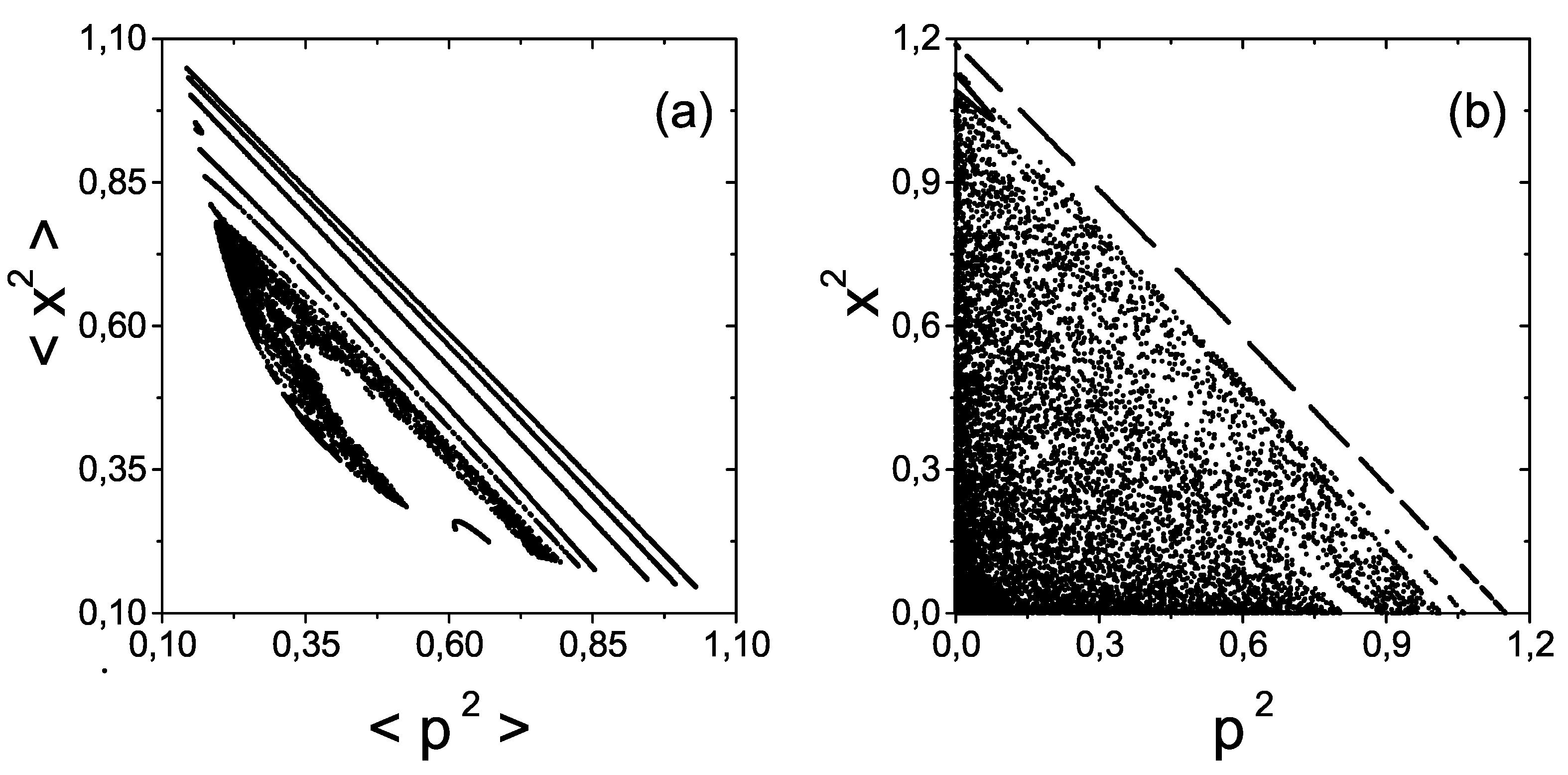
In [18], it was also shown that, by increasing $E_{\mathrm{r}}$ (for example, decreasing I), the system passes through the three zones: a quasiquantal zone, a transitional zone, and a classical zone (see Figures 1 and 2 in [18]). As $E_{\mathrm{r}}$ increases, eventually, chaos emerges in the transitional zone augmenting notably in the classical zone. This is a phenomenon of semi-classical nature, since the classical dynamics-stage has, obviously, not been reached so far. Note the coexistence of the uncertainty principle with chaos and that, having $\widehat{\rho }\left(t\right)$, one can know the time dependence of any expectation value via Equation (7). On the other hand, the analogous classical system is chaotic. Both cases are shown in Figure 1.

5. Results Regarding the Classical Limit

In [18], the classical limit was studied numerically. In the present paper, our attention is focused on a particular instance of the limit $E_{\mathrm{r}}\to \infty$ to be scrutinized in analytic fashion. To this end, let us concentrate on the limit $I\to 0$ of the density operator (6). This entails keeping the values of both E and ${\omega }_{\mathrm{q}}$ fixed in the dimensionless quantity $E_r=\left|E\right|/\sqrt{I{\omega }_{\mathrm{q}}}$ while diminishing I. Remember that both E and I are motion invariants; thus, $I\to 0$ entails $E_{\mathrm{r}}\to \infty$.

One needs the relation between the mean values and Lagrange multipliers. From Equation (7), one gets:

$$\begin{array}{ccc}\hfill I_{\lambda }\langle {\widehat{x}}^2\rangle & =& \sqrt{I}{\lambda }_2,\hfill \end{array}$$

(12a)

$$\begin{array}{ccc}\hfill I_{\lambda }\langle {\widehat{p}}^2\rangle & =& \sqrt{I}{\lambda }_1,\hfill \end{array}$$

(12b)

$$\begin{array}{ccc}\hfill I_{\lambda }\langle \widehat{L}\rangle & =& -2\sqrt{I}{\lambda }_3.\hfill \end{array}$$

(12c)

Using Equations (7) and (11) along with Equation (12), one finds an important relation,

$$I_{\lambda }=\frac{1}{2\hslash }ln\left(\frac{\sqrt{I}+\frac{\hslash }{2}}{\sqrt{I}-\frac{\hslash }{2}}\right),$$

(13)

which relates $I_{\lambda }$ with I. This result was already obtained in [18] using a different approach.

Let us now return to the classical limit. In this limit, one has to respect the restriction (5), i.e., confronting only two possible ways (both ways are correct). The first way is to scrutinize the $\hslash \to 0$ calculation. However, the following difficulties are encountered.

• First, an a priori natural one: take $\hslash \to 0$ and, then, $I\to 0$. However, this way does not suit the present study purposes. Classical statistics and quantum statistics, both are compatible with Equation (5) for any $\hslash >0$ (in addition, in classical case, $\hslash =0$ is possible). Therefore, by taking the limit $\hslash \to 0$, the statistical aspect of the problem is not eliminated, but only converts the quantum statistics to the classical statistics. Therefore, the limit $I\to 0$ cannot be taken within the quantum context. However, some interesting results can be found in the associated calculations.
  In the $\hslash \to 0$ limit, the density matrix (9) adopts the form,

  $$\rho =\frac{\mathcal{I}}{Tr\left[\mathcal{I}\right]},$$

  (14)

  where $\mathcal{I}$ is the identity matrix. Then, one has:

  $$\underset{\hslash \to 0}{lim}{I}_{\lambda }=\frac{1}{2\sqrt{I}},$$

  (15)

  as a result of

  $$\underset{\hslash \to 0}{lim}\hslash I_{\lambda }=0,$$

  (16)

  where Equation (13) is employed. Equation (14) represents the maximally mixed density matrix with the diagonal elements $1/n$, $n\epsilon \mathcal{N}$ (the set of natural numbers), $n\to \infty$. Such matrix is the result of a decoherence process. This way one obtains a statistical quantum limit. The limit $I\to 0$ would entail classicality and cannot be taken now. To better understand the issue, an analysis within classical statistics is considered in Appendix A.
• Proceed now to affect, first, the limit $I\to {\hslash }^2/4$, i.e., take the system to its quantum minimum value and then let $\hslash \to 0$. This choice respects the restriction (5) and constitutes the correct method. According to Equations (11)–(13), one has:

  $$\begin{array}{ccc}\hfill \underset{\hslash \to 0}{lim}(\underset{I\to {\hslash }^2/4}{lim}{I}_{\lambda })& =& \infty ,\hfill \end{array}$$

  (17a)

  $$\begin{array}{ccc}\hfill \underset{\hslash \to 0}{lim}(\underset{I\to {\hslash }^2/4}{lim}\hslash I_{\lambda })& =& \infty ,\hfill \end{array}$$

  (17b)

  $$\begin{array}{ccc}\hfill \underset{\hslash \to 0}{lim}(\underset{I\to {\hslash }^2/4}{lim}{\lambda }_i)=\infty ,& & i=0,1,2,\hfill \end{array}$$

  (17c)

  $$\begin{array}{ccc}\hfill \underset{\hslash \to 0}{lim}(\underset{I\to {\hslash }^2/4}{lim}|{\lambda }_3\left|\right)& =& \infty .\hfill \end{array}$$

  (17d)

Note that, in the first instance, when I tends towards its possible minimum value of ${\hslash }^2/4$, $\rho$ (Equation (9)) tends towards its ground state. Thus, considering the pseudo-generalized temperature $1/I_{\lambda }$, one ascertains that $1/I_{\lambda }\to 0$. Let us remark that $I_{\lambda }$ depends on both the classical variables and the initial conditions for the eigenvalues. Note that the results obtained hold also for $\hslash \to 0$.

From Equation (17c), one can see that $exp(-{\lambda }_0)\to \infty$. However, closer scrutiny of the asymptotic behavior of ${\lambda }_0$ in Equation (11) ascertains that $exp(-{\lambda }_0)\sim exp(\hslash I_{\lambda })$. Thus, the eigenvalues (10) tend towards asymptotic values of the form $exp(-2n\hslash I_{\lambda })$, $n=0,1,2$, etc.

Keeping in mind Equation (17b), one finds the classical limit of $\rho$ given by Equation (9). Thus, at the classical limit, $\rho$ (in its eigen-basis) is represented by the associate density matrix,

$$\mathcal{R}\left(t\right)=\left(\begin{array}{c}100\dots \\ 000\dots \\ 000\dots \\ ⋮\end{array}\right).$$

(18)

Thus, one finds that the classical limit is represented by a pure-state density matrix. This is rather surprising.

As shown in Figures 1 and 2 of [18], not only the classical features of the semiclassical evolution are represented by a mixed quantum density, matrix but also the purely classical results with $I=0$ are masked by a pure-state density matrix. In the former case, a semi-classical chaos is obtained; in the latter case, a totally classical chaos is obtained [18]. The expectation values $\langle {\widehat{X}}^n{\widehat{P}}^m\rangle$ are null at all times, thus being of a trivial classical nature. Furthermore, the eigenvalues of the set (${\widehat{x}}^2$, ${\widehat{p}}^2$, and $\widehat{L}$) evolve asymptotically with the classical equations corresponding to the classical counterpart of the quantum Hamiltonian (4). Any other asymptotic value of a given eigenvalue can be calculated using Equations (7) and (8).

As a proof of the correctness of results obtained here, it is enough to note that I calculated with $\rho \left(t\right)$, given by (18), vanishes. Denoting the ground state by $|0$>, one gets: <$0|{\widehat{X}}^2|0$$>$$=$<$0|{\widehat{P}}^2|0$$>$$=\underset{\hslash \to 0}{lim}\hslash /2$ and <$0|\widehat{L}|0$$>$$=0$, so that $I=0$. Moreover, via the maximum entropy expression, $S\left(\widehat{\rho }\right)=-\mathrm{Tr}[\widehat{\rho }ln\widehat{\rho }]={\lambda }_0+{\sum }_{i=1}^3{\lambda }_i\langle {\widehat{O}}_i\rangle$, one obtains for the entropy:

$$S={\lambda }_0+2I_{\lambda }\sqrt{I},$$

(19)

an increasing monotonic function of I with asymptotic value $S=0$, as expected for a pure state. This way, the density operator smoothly becomes less and less mixed, as soon as I tends towards zero, until the density operator is represented by a pure-state density matrix.

6. Conclusions

In this paper, the classical limit of a density operator, $\rho$, is investigated being associated with a known nonlinear semi-classical system that possesses both classical and quantum interacting degrees of freedom. This study continues the earlier invetigation [18] where $\rho$ was considered in the context of incomplete prior information.

In [18], three well-delimited and different zones towards the classical limit were numerically detected. These zones were found to be characterized by the dimensionless parameter $E_{\mathrm{r}}=\left|E\right|/\left(\sqrt{I}{\omega }_{\mathrm{q}}\right)$, con $E_{\mathrm{r}}\to \infty$, with E being the total energy and I being a dynamical invariant intimately linked to the uncertainty principle. A quasiclassical zone, a transitional zone, and a classical zone were determined. As $E_{\mathrm{r}}$ increases, the complexity augments and, eventually, a chaos emerges. This phenomenon is of a semi-classical nature. On the other hand, the analogous classical system is chaotic.

In the prsent paper, an analytical treatment is performed for a special case of the limit $E_{\mathrm{r}}\to \infty$. This entails keeping the E and ${\omega }_{\mathrm{q}}$ values fixed while diminishing I.

Two possible ways were contemplated to perform the study. The first way is to perform the $\hslash \to 0$ calculation. Some difficulties encountered in such instance are discussed.

The second way turned out to be both correct and coherent. It consists of taking, first, limit $I\to {\hslash }^2/4$ and approaching the minimum I value that quantum mechanics permits. A posteriori, one deals with the limit $\hslash \to 0$. In quite a counterintuitive expectation, one stumbles on an asymptotic density matrix, $\mathcal{R}$, corresponding to a pure state (18); the latter is shown to adequately describe classical features. Indeed, the eigenvalues of the set evolve asymptotically with the classical equations corresponding to the classical counterpart of the Hamiltonian. In particular, it is conclusively shown that $\mathcal{R}$ describes the classical chaos.

References

- Brack, M.; Bhaduri, R.K. Semiclassical Physics; CRC Press: Boca Raton, FL, USA, 2019. [Google Scholar]
- Struyve, W. Semi-classical approximations based on Bohmian mechanics. Int. J. Mod. Phys. A 2020, 35, 2050070. [Google Scholar] [CrossRef]
- Giulini, D.; Joos, E.; Kiefer, C.; Kupsch, J.; Stamatescu, O.; Zeh, H.D. Decoherence and the Appearance of the Classical World in Quantum Theory; Springer: Berlin, Germany, 2003. [Google Scholar]
- Arndt, M.; Hornberger, K.; Zeilinger, A. Probing the limits of the quantum world. Phys. World 2005, 18, 35–40. [Google Scholar] [CrossRef]
- Zeh, H.D. Why Bohms quantum theory? Found. Phys. Lett. 1999, 10, 197–200. [Google Scholar] [CrossRef] [Green Version]
- Bloch, F. Nuclear Induction. Phys. Rev. 1946, 70, 460–474. [Google Scholar] [CrossRef]
- Milonni, P.; Shih, M.; Ackerhalt, J.R. Chaos in Laser-Matter Interactions; World Scientific Publishing Co.: Singapore, 1987. [Google Scholar]
- Ring, P.; Schuck, P. The Nuclear Many-Body Problem; Springer: Berlin, Germany, 1980. [Google Scholar]
- D’Alessio, L.; Kafri, Y.; Polkovnikov, A.; Rigol, M. From quantum chaos and eigenstate thermalization to statistical mechanics and thermodynamics. Adv. Phys. 2016, 65, 239–362. [Google Scholar] [CrossRef] [Green Version]
- Ribeiro, R.F.; Burke, K. Deriving uniform semiclassical approximations for one-dimensional fermionic systems. J. Chem. Phys. 2018, 148, 194103. [Google Scholar] [CrossRef] [PubMed]
- Gravielle, M.S.; Miraglia, J.E. Semiquantum approach for fast atom diffraction: Solving the rainbow divergence. Phys. Rev. A 2014, 90, 052718. [Google Scholar] [CrossRef] [Green Version]
- Barker, J.; Bauer, G.E.W. Semiquantum thermodynamics of complex ferrimagnets. Phys. Rev. B 2019, 100, 140401(R). [Google Scholar] [CrossRef] [Green Version]
- Kowalski, A.M.; Rossignoli, R. Nonlinear dynamics of a semiquantum Hamiltonian in the vicinity of quantum unstable regimes. Chaos Solitons Fractals 2018, 109, 140–145. [Google Scholar] [CrossRef] [Green Version]
- Cooper, F.; Dawson, J.; Habib, S.; Ryne, R.D. Chaos in time-dependent variational approximations to quantum dynamics. Phys. Rev. E 1998, 57, 1489–1498. [Google Scholar] [CrossRef] [Green Version]
- Kowalski, A.M.; Plastino, A.; Proto, A.N. Classical limits. Phys. Lett. A 2002, 297, 162–172. [Google Scholar] [CrossRef]
- Kowalski, A.M.; Martín, M.T.; Plastino, A.; Rosso, O.A. Bandt-Pompe approach to the classical-quantum transition. Phys. D 2007, 233, 21–31. [Google Scholar] [CrossRef]
- Kowalski, A.M.; Martin, M.T.; Plastino, A.; Judge, G. Kullback-Leibler Approach to Chaotic Time Series. SOP Trans. Theor. Phys. 1 2014, 3, 40–49. [Google Scholar]
- Kowalski, A.M.; Plastino, A. Chaotic density matrix in the classical limit. Phys. Lett. A 2020, 384, 126450. [Google Scholar] [CrossRef]
- Coddington, E.; Levinson, N. Theory of Ordinary Differential Equations; McGraw-Hill Publishing: New York, NY, USA, 1976. [Google Scholar]
- Katz, A. Principles of Statistical Mechanics; Freeman: San Francisco, CA, USA, 1967. [Google Scholar]
- Alhassid, Y.; Levine, R.D. Connection between the maximal entropy and the scattering theoretic analyses of collision processes. Phys. Rev. A 1978, 18, 89–116. [Google Scholar] [CrossRef]
Figure 1.
Poincaré surfaces for the system total energy, (in arbitrary units), the time t-dependent classical variable of the model Hamiltonian and, respectively, the Hamiltonian quantum and classical masses, , where is the quantum system frequency and e is the charge. (a) Quantum operators vs. for the relative energy (a pure number) because is a ratio of two energies. . The Poincare surface is enclosed by the curves and corresponding to the uncertainty principle. Here, one can observe the coexistence of a chaos with the uncertainty principle that represents semiquantum chaos. (b) Classical functions vs. , corresponding to and (see text), which coincides with the classical instance . The surface is bounded only by . Here, one can visually detect the classical chaos presence in the graphs. The accuracy of the results were checked by verifying the constancy with time of the dynamical invariants E and I (with precision of ).
Publisher’s Note: MDPI stays neutral with regard to jurisdictional claims in published maps and institutional affiliations. |
© 2021 by the authors. Licensee MDPI, Basel, Switzerland. This article is an open access article distributed under the terms and conditions of the Creative Commons Attribution (CC BY) license (https://creativecommons.org/licenses/by/4.0/).
Share and Cite
MDPI and ACS Style
Kowalski, A.M.; Plastino, A.; Gonzalez, G. Classical Chaos Described by a Density Matrix. Physics 2021, 3, 739-746. https://0-doi-org.brum.beds.ac.uk/10.3390/physics3030045
AMA Style
Kowalski AM, Plastino A, Gonzalez G. Classical Chaos Described by a Density Matrix. Physics. 2021; 3(3):739-746. https://0-doi-org.brum.beds.ac.uk/10.3390/physics3030045
Chicago/Turabian StyleKowalski, Andres Mauricio, Angelo Plastino, and Gaspar Gonzalez. 2021. "Classical Chaos Described by a Density Matrix" Physics 3, no. 3: 739-746. https://0-doi-org.brum.beds.ac.uk/10.3390/physics3030045