Description of Nonlinear Vortical Flows of Incompressible Fluid in Terms of a Quasi-Potential


1
Centre for Ocean Energy Research, Maynooth University, Co. Kildare, W23 F2H6 Maynooth, Ireland
2
School of Sciences, University of Southern Queensland, West St., Toowoomba, QLD 4350, Australia
3
Department of Applied Mathematics, Nizhny Novgorod State Technical University n.a. R.E. Alekseev, 24 Minin St., 603950 Nizhny Novgorod, Russia
*
Author to whom correspondence should be addressed.
Physics 2021, 3(4), 799-813; https://0-doi-org.brum.beds.ac.uk/10.3390/physics3040050
Submission received: 9 August 2021
/
Revised: 13 September 2021
/
Accepted: 13 September 2021
/
Published: 22 September 2021
(This article belongs to the Special Issue Dedication to Professor Michael Tribelsky: 50 Years in Physics)
Abstract
:As it was shown earlier, a wide class of nonlinear 3-dimensional (3D) fluid flows of incompressible viscous fluid can be described by only one scalar function dubbed the quasi-potential. This class of fluid flows is characterized by a three-component velocity field having a two-component vorticity field. Both these fields may, in general, depend on all three spatial variables and time. In this paper, the governing equations for the quasi-potential are derived and simple illustrative examples of 3D flows in the Cartesian coordinates are presented. The generalisation of the developed approach to the fluid flows in the cylindrical and spherical coordinate frames represents a nontrivial problem that has not been solved yet. In this paper, this gap is filled and the concept of a quasi-potential to the cylindrical and spherical coordinate frames is further developed. A few illustrative examples are presented which can be of interest for practical applications.
1. Introduction
A great success in the solution of fluid dynamic problems is associated with the reduction of a primitive set of hydrodynamic equations to only one equation for some scalar function, e.g., velocity potential or stream function [1,2,3,4,5]. It has been shown in [6,7] that the class of exactly solvable hydrodynamic problems can be widened by introducing one more scalar function dubbed the quasi-potential. The starting point for the introduction of the quasi-potential is the condition of incompressibility of a fluid: , where is the velocity field. This condition allows us to introduce a vector-potential such that automatically satisfies this equation. However, there is a gauge invariance in the choice of the vector-potential as it is defined up to the gradient of any scalar function of spatial variables x, y and z because . Therefore, the addition of the gradient of an arbitrary function to the vector-potential, , does not affect the velocity field . Due to the freedom of choice of an arbitrary function , one of the components of the vector-potential can be eliminated. Therefore, without loss of generality, the vector potential can be chosen consisting of two components only. It does not matter which component is eliminated in the Cartesian rectilinear coordinates because vector differential operations are symmetrical with respect to all spatial variables. However, it is not the case in curvilinear coordinates, in particular, in cylindrical or spherical coordinates. In any case, an arbitrary 3-dimensional velocity field can be described, in general, by two-component vector-potential, i.e., by two scalar functions—the corresponding components of the vector-potential. If there is any additional link between these two components, then the description of a fluid flow can be done in terms of only one scalar function. The governing equation for the corresponding scalar function can be derived from the primitive Navier–Stokes equation. This approach has been exploited in [6,7] in Cartesian coordinates and illustrated by nontrivial examples of fluid flows.
In this paper, fluid flows in the cylindrical and spherical coordinates are considered and it is shown how the quasi-potential can be introduced when one of the components of the vector-potential is eliminated and two other components are linked with each other. Illustrative examples, which demonstrate three-dimensional velocity field with only two components of vorticity, are provided.
2. Governing Equations and Quasi-Potential in Cylindrical Coordinates
2.1. Case 1—Vector-Potential Does Not Contain the Radial Component
Consider first the case when the vector-potential does not contain the radial component which is eliminated by the appropriate choice of function . Then, it can be presented as , where and are functions of time and all spatial variables. Here is the azimuthal angle, and and are the unit vectors. The velocity and vorticity fields for such a vector-potential are:
respectively, where .
Consider a particular class of fluid flows having only two components of the vorticity, the - and z-components. For such a class of fluid motion, one has the following differential link between the functions and :
Substitute then the expressions for and in the Navier–Stokes equation in the Helmholtz form (4) [1]:
Bearing in mind that thanks to the condition (3), the r-component of the vorticity is zero, one obtains from Equation (4):
Let us introduce function such that
Then, the left-hand side of Equation (5) reduces to the Jacobian of two functions and S with respect to the variables and z. As well known, if the Jacobian is zero then, the functions are related by an arbitrary function. In our case this means that J, so that , where G is an arbitrary function of S, r and time t. Using the definition of function (see after Equation (2)) and Equation (6), one obtains:
where is the quasi-potential, and prime stands for differentiation with respect to the corresponding variable indicated by a subscript.
In terms of the quasi-potential, the velocity and vorticity fields can be presented, respectively, as:
By substitution of these expressions into two other components (the - and z-components) of the Helmholtz Equation (4), after some manipulations (see Appendix A) the equations reduce:
where is an arbitrary function of the arguments.
In the particular case of , the quasi-potential becomes the conventional hydrodynamic velocity potential. Equation (7) reduces to the Laplace equation, Equation (10) disappears, and vorticity vanishes. In general, the main equations to be solved simultaneously are Equations (7) and (10) with two arbitrary functions and . As there is big freedom in the choice of these functions, one obtains a good perspective to construct exact solutions to hydrodynamic equations and accommodate them to practical needs.
2.2. Case 2—Vector-Potential Does Not Contain the Azimuthal Component
Consider now the case when the vector potential has only r- and z-components: . In this case, the velocity and vorticity fields become:
respectively, where .
Let us consider such a class of fluid motion which does not contain the -component of vorticity. In this case, there must be a relationship between functions and such that . Then, the -component of the Helmholtz Equation (4) reduces to:
The left-hand side of this equation reduces to the Jacobian on variables r and z as soon as such function is introduced that
Then, from Equation (13) one obtains: , where G is an arbitrary function of S, and t. Recalling the definition of function in terms of and and introducing a quasi-potential such that , Equation (13) reduces to:
In terms of quasi-potential the velocity and vorticity fields read, respectively:
In the case of a perfect fluid (), two other components, the r- and z-components, of the Helmholtz Equation (4) after simple but long manipulations similar to those presented in Appendix A can be reduced to only one equation:
where is an arbitrary function of the arguments.
In the particular case of , the quasi-potential becomes a conventional hydrodynamic velocity potential. Equation (15) reduces to the Laplace equation, Equation (18) vanishes, the velocity field becomes potential, and the vorticity field vanishes. In general, the main equations to be solved simultaneously for are Equations (15) and (18) with given functions , and . Despite the more complex character of these equations, the freedom of choice of arbitrary functions allows one to obtain again a good perspective to construct exact solutions to hydrodynamic equations and accommodate them to practical needs. Unfortunately, in the case of a viscous fluid () the introduction of a quasi-potential does not help to simplify the basic Equation (4).
Example of a Vortical Flow Illustrating Case 2
To illustrate this case, let us assume that function , where is a constant. One can readily verify that the following quasi-potential,
satisfies Equations (15) and (18). Then, the velocity and vorticity fields read, respectively:
This solution describes stationary vortical flow periodic in azimuthal coordinate and has two components of vorticity. When , the velocity and vorticity fields vanish, whereas when , the flow becomes potential with the zero vorticity.
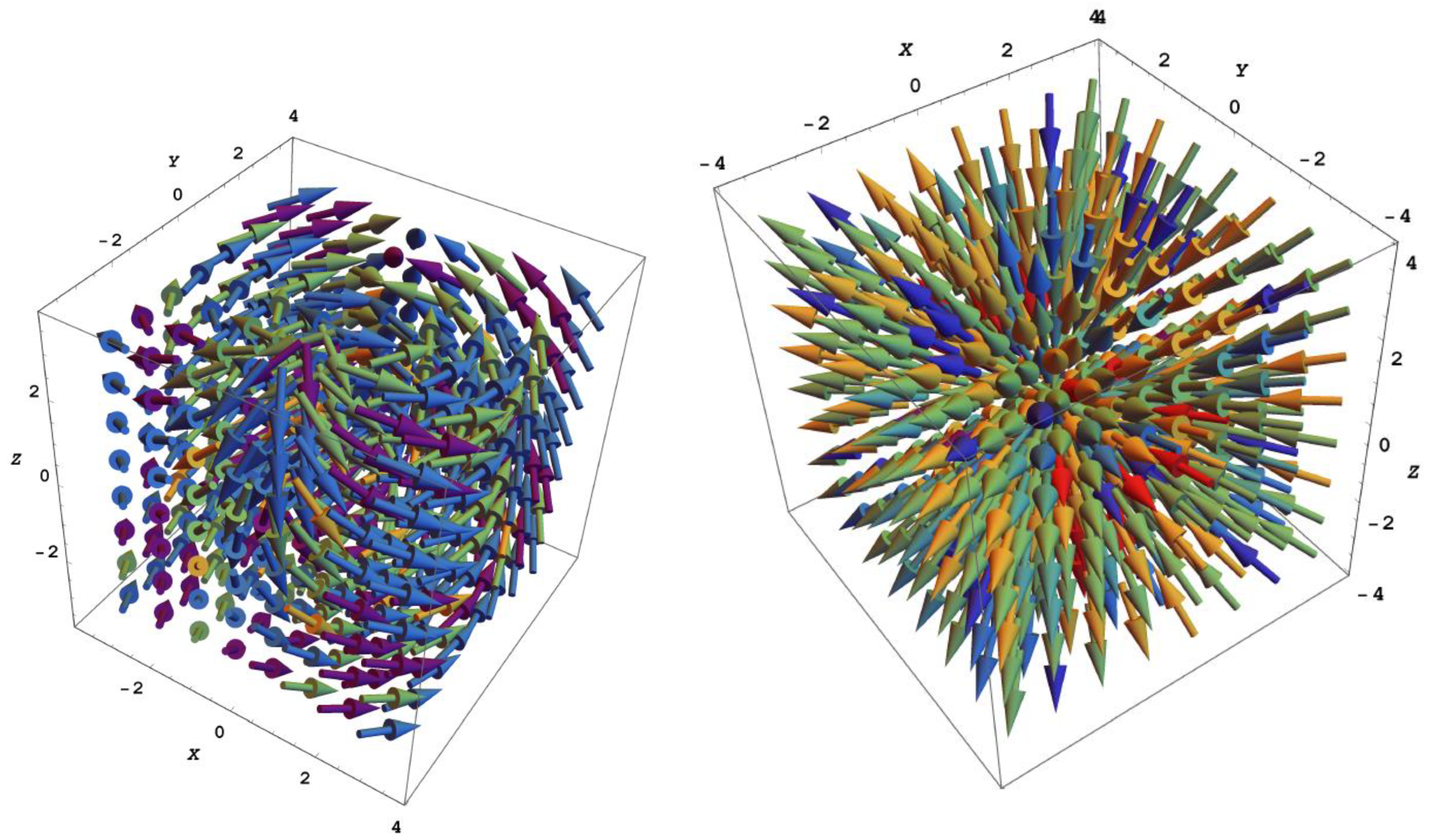
In Cartesian coordinates, both the velocity and vorticity fields have all three components:
where ;
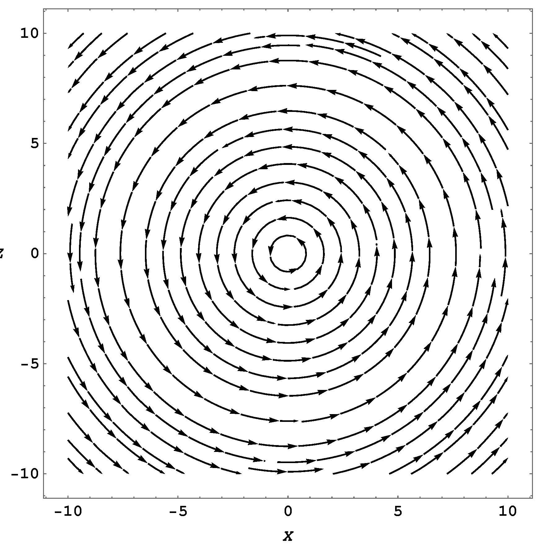
Figure 1 illustrates the velocity and vorticity fields as per Equations (22) and (23). The modulus of the velocity field is:
Furthermore, the modulus of the vorticity field is:
2.3. Case 3—Vector-Potential Does Not Contain the Axial Component
Consider at last the case when the vector potential has only r- and -components and can be presented through the function and in the following way: . In this case the velocity and vorticity fields become, respectively:
where .
Assuming that the z-component of the vorticity is zero, one obtains the following relationship between the function and :
By substitution the expressions for the velocity and vorticity in the Helmholtz Equation (4), one obtains:
Let us introduce function such that
Then, the left-hand side of Equation (5) reduces to the Jacobian of two functions and S with respect to the variables r and . Omitting the details which are similar to those presented in two previous section, one finds: , where G is an arbitrary function of S, z and t. Using then the definition of function (see Equation (27)) and Equation (30), one obtains:
where the quasi-potential is .
In terms of the quasi-potential, the velocity and vorticity fields can be presented, respectively, as:
By substitution of these expressions into two other components (the r- and -components) of the Helmholtz Equation (4) and neglecting viscosity (), after some manipulations, similar to those presented in the Appendix A, the equations reduce to only one equation:
where is an arbitrary function of the arguments.
In the particular case of , the quasi-potential becomes the conventional hydrodynamic velocity potential. Equation (31) reduces to the Laplace equation, Equation (34) disappears, and vorticity vanishes. In general, the main equations to be solved simultaneously are Equations (31) and (34) with two arbitrary functions and . There is again a big freedom in the choice of these functions, so that one can obtain a good perspective to construct exact solutions to hydrodynamic equations and accommodate them to practical needs. Unfortunately, in the case of a viscous fluid (), the introduction of a quasi-potential does not help to simplify the basic Equation (4).
Example of a Vortical Flow Illustrating Case 3
Consider now an example of the vortical flow for the third case when the vector potential has only r- and -components in cylindrical coordinates. Let us assume that , where is a constant. One can readily verify that the following quasi-potential,
satisfies Equations (31) and (34). Then, the velocity and vorticity fields read, respcetively:
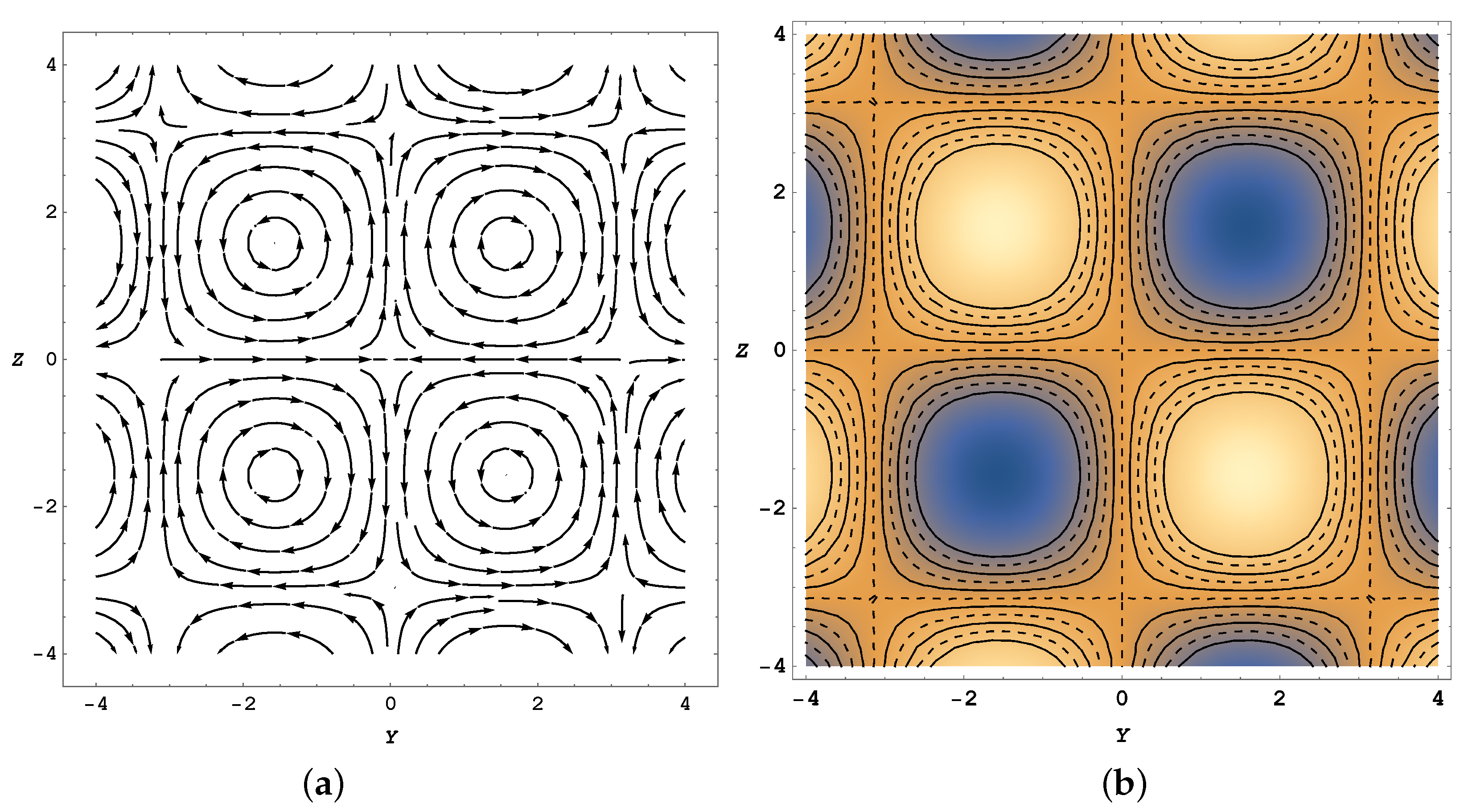
This solution describes non-viscous stationary fluid flow. The vector fields and are periodic in and z. In Cartesian coordinates, the velocity field becomes two-component:
whereas the vorticity field has only one x-component:
Both these fields do not depend on x and therefore can be described by the conventional stream function , so that the velocity components are:
For purely imaginary , the quasi-potential reduces to the conventional hydrodynamic potential, and the fluid field becomes potential with zero vorticity:
Thus, in general, this example describes a vortical flow double periodic in the plane. Figure 2 illustrates the velocity and vorticity fields for when y and z vary in the range .
In this Section, only two simple examples have been presented to illustrate vortical flows of inviscid fluid flows. As one can see already from these two examples, the introduction of quasi-potentials allows us to construct exact solutions for fairly complex vortical flows in cylindrical coordinates. The transformation of a two-component vorticity field акщь cylindrical to Cartesian coordinates can lead to either one-component or three-component vorticity fields. There is no regular method to construct three-component vortical flows in Cartesian coordinates, whereas the developed theory allows us to find some exact solutions for such flows in terms of the quasi-potential.
3. Governing Equations and Quasi-Potential in Spherical Coordinates
The derivation of basic equations for the spherical case are similar but not the same to that presented in Section 2. Therefore, the derivation of the corresponding equations is described only briefly.
3.1. Case 1—Vector-Potential Does Not Contain the Radial Component
Consider the case when the vector-potential does not contain the component and reads: where is the polar angle, and F1 and F2 are functions of time and all spatial variables. The velocity and vorticity fields for such vector-potential are:
respectively, where .
Consider again a particular class of fluid flows with the zero first component of the vorticity. Then, the relationship between functions and :
Let us introduce function S such that
Then Equation (44) takes a form of the Jacobian of two functions, with respect to the variables and . This gives , where G is an arbitrary function of the arguments. Using the definition of function and Equation (45), one can reduce this relationship to the equation:
where the quasi-potential is defined by the equation , and is the Laplacian in spherical coordinates. This equation can be rewritten in the form:
The expressions for the velocity and vorticity fields in terms of the quasi-potential, are, respectively:
Then, from the other two components of the Helmholtz Equation (4) neglecting the viscosity (), one obtains:
where is an arbitrary function of the arguments. Choosing , one obtains the expressions for the potential fluid flow with the zero vorticity and .
The Illustrative Example
Let us construct the illustrative example of a stationary flow for this case with the following choice of functions and :
The velocity and vorticity fields with such choice of functions are, respectively:
These fields in the Cartesian coordinates look as follows:
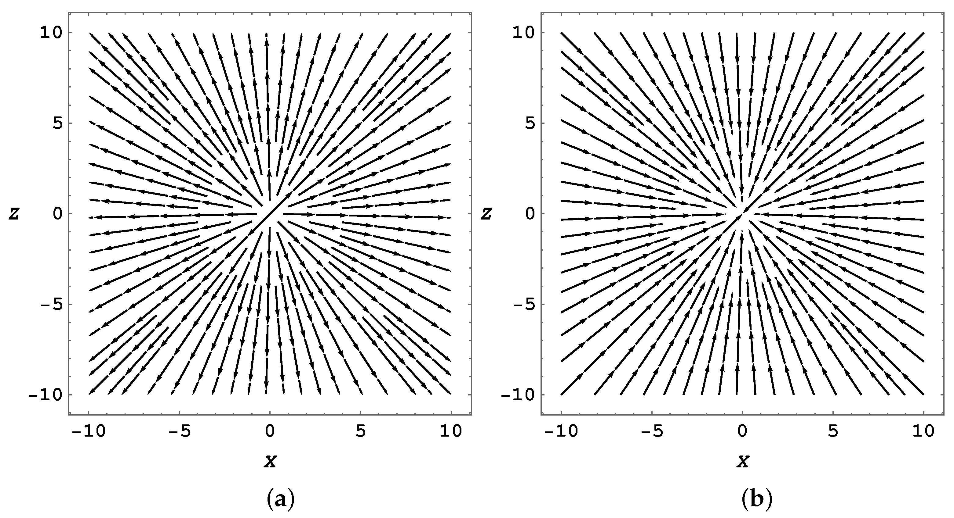
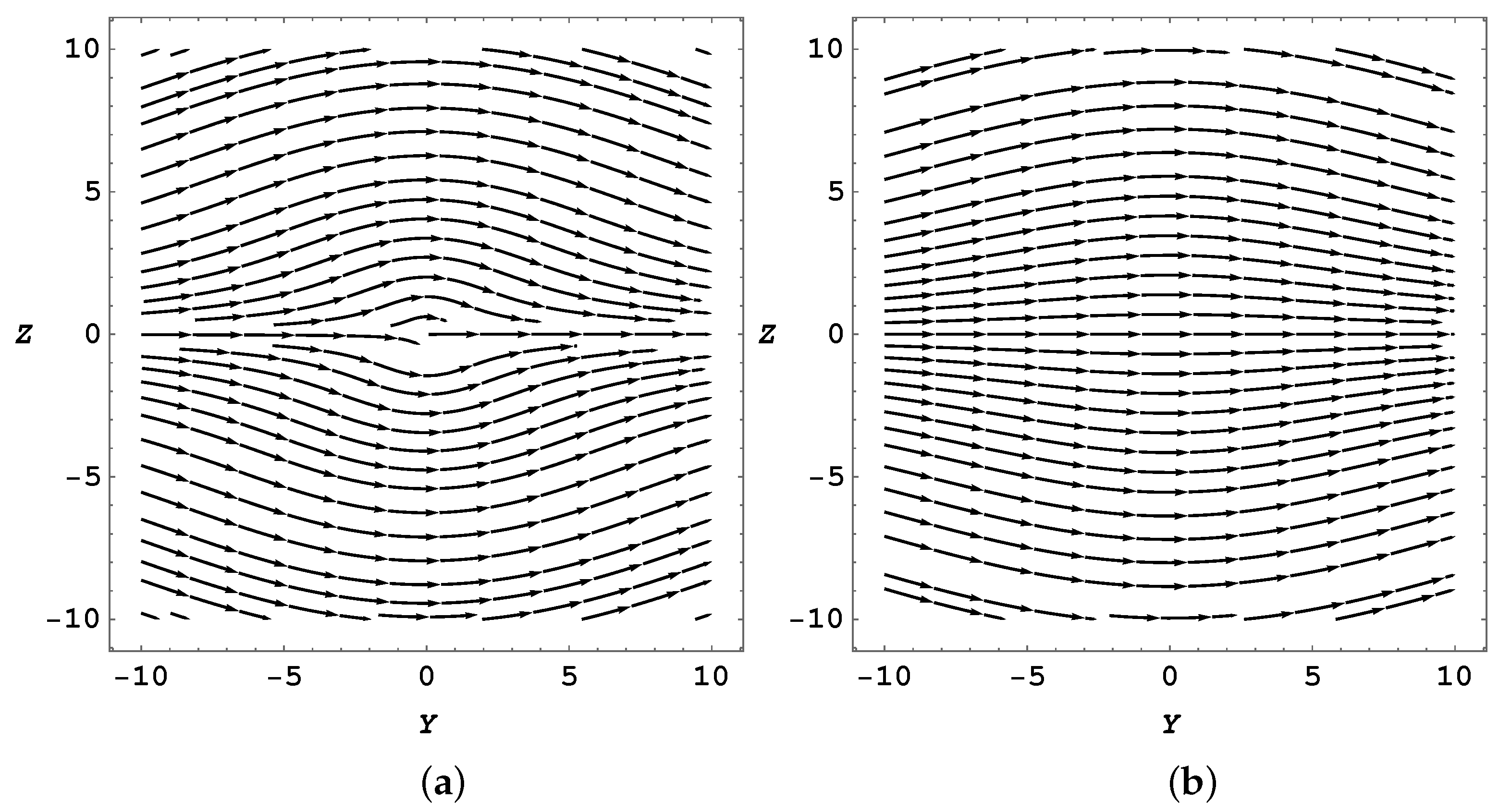
Figure 3 illustrates the velocity field in the planes and .
3.2. Case 2—Vector-Potential Does Not Contain the Azimuthal Component
Consider now the case when the vector-potential does not contain the azimuthal component and reads: , where and are functions of time and all spatial variables. The velocity and vorticity fields for such vector-potential read:
respectively, where .
Considering such a class of fluid flows which do not contain the -component of the vorticity, one obtains a relationship between the functions and :
Then, from the -component of the Helmholtz Equation (4) one obtains:
Introducing function such that
Equation (58) can be presented in the Jacobian form:
This implies that , where G is an arbitrary function of the arguments. Using the definition of function (see Equation (56)) and the relationship (57) between functions and , one finally derives the static equation for the quasi-potential :
Another equation, describing the time dependence of , can be obtained from two other components (r- and -components) of the Helmholtz Equation (4). Omitting the details, which are similar to those shown in Appendix A, for the perfect fluid (), this equation reads:
where is an arbitrary function of the arguments.
In terms of quasi-potential the velocity and vorticity fields are, respectively:
Choosing , one obtains the expressions for the potential fluid flow with the zero vorticity and .
3.3. Case 3—Vector-Potential Does Not Contain the Polar Component
Consider, at last, the case when the vector-potential does not contain the polar component and reads: , where and are functions of time and all spatial variables. The velocity and vorticity fields for such vector-potential are, respectively:
where .
Consider now a particular class of fluid flows with the zero polar component of the vorticity. Then, one obtains the relationship between functions and :
Then, from the -component of the Helmholtz Equation (4) one obtains:
This implies that , where G is an arbitrary function of the arguments. Using the definition of function (see Equation (66) and the relationship between functions and (67), one finally obtains the static equation for the function S:
where quasi-potential is , and is the Laplacian in spherical coordinates.
Another equation, describing time dependence of S, can be obtained from two other components (r- and -components) of the Helmholtz Equation (4) with . Omitting the details, which are similar to those presented in Appendix A, the final expression is:
Then, the formulae for the velocity and vorticity fields are, respectively:
These formulae exhaust all possible versions of introduction of a quasi-potential in spherical coordinates. No an illustrative example is found for this case but let believe that this may be possible and, hopefully, an example will be found in the future, moreover, it can be of a practical interest.
4. Conclusions
Thus, in this paper it has been demonstrated that the introduction of a proper quasi-potential is possible in the cylindrical and spherical geometry albeit it is not a trivial generalisation of the quasi-potential theory developed in Refs. [6,7]. The quasi-potential approach helps one to construct exact solutions describing fairly complex class of three-dimensional velocity fields with two-component vorticity fields. After transformation from the curvilinear coordinates to the Cartesian coordinates, the velocity and vorticity fields can become fairly complex containing all three components of velocity and vorticity. In the particular cases, the quasi-potential theory reduces to the conventional potential theory or to the theory of a vortex flow based on the introduction of a stream-function. Our preliminary study shows that the quasi-potential approach can be used also in other curvilinear coordinates however, the basic equations and formulae for the velocity and vorticity fields become fairly complex and not so illustrative. Summarising the results obtained in this paper and in Refs. [6,7], one can see that the traditional potential theory describes fluid flows with zero vorticity; the stream-function approach allows us to describe flows with only one component of vorticity; and the introduction of a quasi-potential allows us to describe flows with two components of vorticity. It can be noted in conclusion that, unfortunately, new ideas in the description of classical hydrodynamics appear seldom. Three relatively recent publications [8,9,10] can be mentioned to illustrate that the development of such ideas leads to the discovery of new non-trivial exact solutions in classical fluid mechanics.
In Appendix B one of the authors of this paper (Y.S.) presents his brief reminiscent about contacts with M. Tribelsky to whose honour this issue is dedicated.
Author Contributions
Conceptualization, Y.S.; methodology, Y.S.; validation, A.E. and Y.S.; formal analysis, A.E.; investigation, A.E. and Y.S.; writing—original draft preparation, A.E.; writing—review and editing, Y.S.; visualization, A.E.; supervision, Y.S. All authors have read and agreed to the published version of the manuscript.
Funding
Y.S. acknowledges the funding of this study provided by the State task program in the sphere of scientific activity of the Ministry of Science and Higher Education of the Russian Federation (project No. FSWE-2020-0007) and the grant of President of the Russian Federation for the state support of Leading Scientific Schools of the Russian Federation (grant No. NSH- 2485.2020.5). The paper was completed when Y.S. was working under the SMRI visiting program at The University of Sydney in March–April 2021. Y.S. is thankful for the provided grant and hospitality of SMRI staff.
Conflicts of Interest
The authors declare no conflict of interests.
Appendix A
The -component of the Helmholtz Equation (4) after substitution the expressions for the velocity (8) and vorticity (9) fields gives:
This equation can be rewritten in the form:
After integration over z this equation reduces to:
where is an arbitrary function of the arguments.
Then, the similar manipulations with the z-component of the Helmholtz Equation (4) lead to the equation:
The left-hand side of Equations (A1) and (A2) are identical; therefore, one can conclude that functions and can depend only on r and t and must be equal. Denoting them by , one obtains Equation (10).
Appendix B
Here, one of the authors, Y.S., presents his reminiscent about friendship contacts with Michael Tribelsky (Misha). We met relatively late, in 2007, when we both worked as Visiting Professors at the Max Planck Institute for the Physics of Complex Systems, Dresden, Germany. We quickly found many commons between us, including age, education, interests, attitude to science and life. One of the attractive Misha’s features is a great sense of humour and an optimistic attitude to life even when it was hard to him. We spent much time in discussions of physical and mathematical problems, as well as stories of science history.
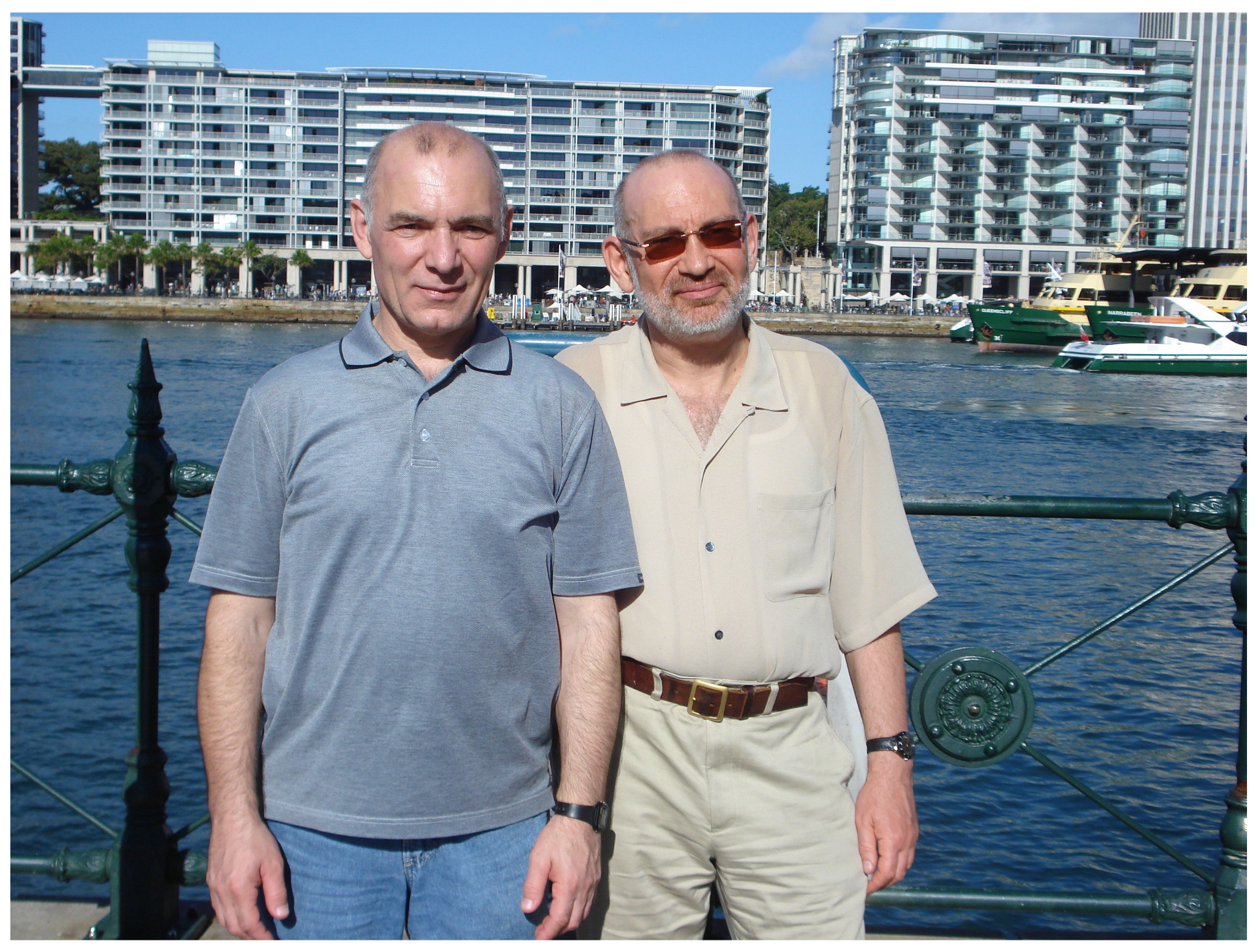
Figure A1.
Yury Stepanyants (left) and Mikhail Tribelsky (right) at the Circular Quay, Sydney, in 2008.
Figure A1.
Yury Stepanyants (left) and Mikhail Tribelsky (right) at the Circular Quay, Sydney, in 2008.

Our contacts continued when Misha visited me in Sydney the next year. I was attracted to them by persistence and perseverance in achieving goals (this is clearly seen from his autobiographical notes presented in this Special Issue). This pertains not only to physical problems but to all aspects of life. I observed how carefully Misha chose the best spots for photography of exotic trees, beautiful buildings, and other objects, taking photos in Sydney when we walked continuously discussing something or disputing on different subjects.
Misha obtained an excellent education in one of the world’s most prestigious physical faculties, namely the one at Lomonosov Moscow State University. He had an opportunity to communicate and jointly work with brilliant world-renowned scientists such as his supervisor Prof. S. Anisimov and then, Profs. Ya. Zeldovich, I. Lifshits, V. Zakharov. He boldly tackled difficult physical problems and found their own, often unconventional solutions to them. I was delighted with his story about solving an important industrial problem for one of the Japanese companies. The problem was related to the calculation of the extinction coefficient in complicated multi-component media. At first, it was not even clear how to approach the task. Still, after persistent reflections, Misha found the key in a relatively short time which caused the admiration of company bosses.
I should also mention Misha’s deep knowledge of computer design and the internal devices of a computer. I had a chance to be convinced that Misha’s level in this field is the same as that (or even higher than that) of professional IT (information technology) experts. Misha generously shared his knowledge with me. More than once, he helped me resolve the difficult issues related to installing and fine-tuning computer programs. It is a pleasure to have such a kind and reliable friend as Misha Tribelsky. I wish him good health and many years of creative work in science.
References
- Lamb, H. Hydrodynamics; Cambridge University Press: Cambridge, UK, 1932. [Google Scholar]
- Milne-Thomson, L.M. Theoretical Hydromechanics; Macmillan Publishers: London, UK, 1960. [Google Scholar]
- Kochin, N.E.; Kibel, I.A.; Roze, N.V. Theoretical Hydromechanics; Interscience Publishers: New York, NY, USA, 1964. [Google Scholar]
- Batchelor, G.K. An Introduction to Fluid Mechanics; Cambridge University Press: Cambridge, UK, 1967. [Google Scholar]
- Landau, L.D.; Lifshitz, E.M. Fluid Mechanics; Pergamon Press: Oxford, UK, 1993. [Google Scholar]
- Stepanyants, Y.A.; Yakubovich, E.I. Scalar description of three-dimensional vortex flows of incompressible fluid. Dokl. Phys. 2011, 56, 130–133. [Google Scholar] [CrossRef]
- Stepanyants, Y.A.; Yakubovich, E.I. The Bernoulli integral for a certain class of non-stationary viscous vortical flows of incompressible fluid. Stud. Appl. Math. 2015, 135, 295–309. [Google Scholar] [CrossRef]
- Makinde, O.D.; Khan, W.A.; Chinyoka, T. New developments in fluid mechanics and its engineering applications. Math. Probl. Eng. 2013, 2013, 797390. [Google Scholar] [CrossRef]
- Yakubovich, E.I.; Zenkovich, D.A. Matrix approach to Lagrangian fluid dynamics. J. Fluid Mech. 2001, 443, 167–196. [Google Scholar] [CrossRef]
- Yakubovich, E.I.; Shrira, V.I. Non-steady columnar motions in rotating stratified Boussinesq fluids: Exact Lagrangian and Eulerian description. J. Fluid Mech. 2011, 691, 417–439. [Google Scholar] [CrossRef]
Figure 1.
Fragments of (a) the velocity field as per Equation (22), and (b) the vorticity field as per Equation (23) for .

Figure 2.
Fragments of (a) the velocity field as per Equation (38), and (b) the density of vorticity field as per Equation (39).

Figure 3.
The velocity field in the planes (a) and (b) as per Equation (54).
Figure 3.
The velocity field in the planes (a) and (b) as per Equation (54).

Figure 4.
The velocity field in the planes (a) and (b) as per Equation (54).
Figure 4.
The velocity field in the planes (a) and (b) as per Equation (54).

Figure 5.
The vorticity field in the -plane as per Equation (54).
Figure 5.
The vorticity field in the -plane as per Equation (54).

Publisher’s Note: MDPI stays neutral with regard to jurisdictional claims in published maps and institutional affiliations. |
© 2021 by the authors. Licensee MDPI, Basel, Switzerland. This article is an open access article distributed under the terms and conditions of the Creative Commons Attribution (CC BY) license (https://creativecommons.org/licenses/by/4.0/).
Share and Cite
MDPI and ACS Style
Ermakov, A.; Stepanyants, Y. Description of Nonlinear Vortical Flows of Incompressible Fluid in Terms of a Quasi-Potential. Physics 2021, 3, 799-813. https://0-doi-org.brum.beds.ac.uk/10.3390/physics3040050
AMA Style
Ermakov A, Stepanyants Y. Description of Nonlinear Vortical Flows of Incompressible Fluid in Terms of a Quasi-Potential. Physics. 2021; 3(4):799-813. https://0-doi-org.brum.beds.ac.uk/10.3390/physics3040050
Chicago/Turabian StyleErmakov, Andrei, and Yury Stepanyants. 2021. "Description of Nonlinear Vortical Flows of Incompressible Fluid in Terms of a Quasi-Potential" Physics 3, no. 4: 799-813. https://0-doi-org.brum.beds.ac.uk/10.3390/physics3040050