Stellar Structure in a Newtonian Theory with Variable G

Abstract

A Newtonian-like theory inspired by the Brans–Dicke gravitational Lagrangian has been recently proposed by us. For static configurations, the gravitational coupling acquires an intrinsic spatial dependence within the matter distribution. Therefore, the interior of astrophysical configurations may provide a testable environment for this approach as long as no screening mechanism is evoked. In this work, we focus on the stellar hydrostatic equilibrium structure in such a varying Newtonian gravitational coupling G scenario. A modified Lane–Emden equation is presented and its solutions for various values of the polytropic index are discussed. The role played by the theory parameter $\omega$, the analogue of the Brans–Dicke parameter, in the physical properties of stars is discussed.

1. Introduction

Are the fundamental constants of physics truly constants? This is a long-standing question, perhaps dating back to the identification of these constants themselves. In physics, we can identify, in particular, four fundamental constants, each one connected with a given theoretical structure: the (reduced) Planck constant, ℏ, which defines the quantum world; c, the speed of light, which is the limit velocity and is related to the relativistic domain; the Newtonian gravitational constant, G, which indicates the presence of the gravitational interaction; $k_B$, the Boltzmann constant related to thermodynamics. The presence of one or more of these constants in a given equation can suggest which sort of phenomena we are dealing with. For example, an equation containing G refers to gravitation. If, in addition, it contains c, one faces a relativistic gravitational structure, such as general relativity. If ℏ is added, then quantum gravity is discussing. A phenomenon that, by its nature, is relativistic and involves gravitation and quantum mechanics and, moreover, has a thermodynamic characteristic will contain these four constants. This is the case, for example, of Hawking radiation in a black hole.

Among these four constants, the gravitational coupling G was the first one to be identified, although it is the one that is known with the poorest precision: its value is determined up to the ${10}^{-4}$ order [1]. This is a consequence of the universality of this fundamental physical interaction, the only one that is rigorously present in all phenomena in nature, and always with an attractive behavior. These features led to the identification of gravity with the innermost nature of space and time: all modern theories interpret the gravitational phenomena as a consequence of spacetime curvature. Moreover, since it is always attractive, it dominates the behavior of large-scale systems, such as in astrophysics and cosmology.

There are very stringent observational and experimental constraints on the variation of G. In spite of these constraints, even a small variation of G with time and/or position may have a significant impact on the cosmological and astrophysical observables. For example, the $H_0$ tension may be highly suppressed if G varies with time [2]. Even the large-scale structure formation process may change substantially if G is not a constant. There are many relativistic theories of gravity that try to incorporate the variation of the gravitational coupling. The traditional paradigm of such a theoretical formulation is the Brans–Dicke theory [3], based on an original proposal made by Dirac, inspired by the large number hypothesis, which singles out some curious coincidences of numbers obtained from the combination of the constants and some functions of time evaluated today, such as the Hubble constant [4,5]. The Brans–Dicke theory is a more complete formulation of theoretical developments made by Jordan using the idea that G may not be a constant. Today, the Horndesky class of theories [6] provides the most general gravitational Lagrangian leading to second-order differential field equations. In most cases, the Horndesky theories incorporate the possibility of a dynamical gravitational coupling.

Even if there exists such a plethora of relativistic theories with varying gravitational coupling, it is not so easy to construct a Newtonian theory with a dynamical G. To our knowledge, the first proposals to incorporate a varying G effect in a Newtonian context were made in Refs. [7,8,9]. For example, in Ref. [8], the implementation of this idea was quite simple: in the Poisson equation, a constant G is replaced by a varying gravitational coupling, a function $G\left(t\right)$. There is no dynamical equation for this new function, whose behavior with time must be imposed ad hoc. A natural choice is to use the Dirac proposal, with

$$\begin{array}{c}\hfill G=G_0\frac{t_0}{t},\end{array}$$

(1)

where $t_0$ is the present age of the universe and $G_0$ is the present value of the gravitational coupling. This Newtonian theory with varying gravitation coupling has no complete Lagrangian formulation, since $G\left(t\right)$ is an arbitrary function.

In a recent paper [10], a new Newtonian theory with varying gravitational coupling has been proposed. The gravitational coupling, now given by a function of time and position, is dynamically determined together with the gravitational potential from a new gravitational Lagrangian. It has been shown that this theory is consistent with the general properties of spherical objects such as stars and, at the same time, its homogeneous and isotropic cosmological solutions can generate an accelerated expansion of the universe.

Of course, one may wonder about the interest in constructing a Newtonian theory with varying G. One can evoke the academic interest of obtaining a complete and consistent Newtonian formulation implementing dynamical gravitational coupling. The Newtonian framework is, in principle, simpler than the relativistic one, so would it be so difficult to give a dynamical behavior to G, something that is, if not trivial, at least perfectly possible in a relativistic context? However, at least two other motivations can be quoted. First, a consistent Newtonian theory with varying G may suggest possible new relativistic structures, such as, for example, the non-minimal coupling of gravity with other fields, in a similar way as the general relativity equations suggested by the Poisson equation. Second, many astrophysical and cosmological problems are more conveniently analyzed in a Newtonian framework, e.g., the dynamics of galaxies, clusters of galaxies and even numerical simulations of large-scale structures. If G is not a constant, it would be beneficial to have a consistent Newtonian theory incorporating this feature.

In this paper, we focus on the stellar structure of non-relativistic stars. This is an important analysis in the context of the theory proposed in [10] since it has been shown that the main difference from the standard Newtonian gravity should manifest within matter distributions.

2. Newtonian Theory with Variable G

In Ref. [10], a Lagrangian for a theory with varying G has been proposed and is reviewed in this Section. The Lagrangian of this new approach is given by

$$\mathcal{L}=\frac{\nabla \psi ·\nabla \psi }{2}-\frac{\omega }{2}(\psi \frac{{\dot{\sigma }}^2}{{\sigma }^2}-c^4\nabla \sigma ·\nabla \sigma )+4\pi G_0\rho \sigma \psi ,$$

(2)

where $G_0$ is a constant, $\psi$ is an equivalent of the ordinary Newtonian potential and $\sigma$ is a new function related to the gravitational coupling. In addition, the parameter $\omega$, which shall be assumed to be constant, is introduced.

A constant with dimensions of velocity, the speed of light c, has been introduced to guarantee that the Lagrangian has the correct physical dimensions. However, no direct mention is made of a relativistic framework in doing so: one has simply borrowed from electromagnetism two fundamental constants, the vacuum electric permissivity ${ϵ}_0$ and magnetic permeability ${\mu }_0$.

In some sense, the above Lagrangian corresponds to the Newtonian version of the relativistic Brans–Dicke theory (in Einstein’s framework). Let us emphasize again that the constant c appears in this Lagrangian for dimensional reasons. This does not mean that this is a relativistic theory since this Lagrangian is invariant under the Galilean group transformations.

Applying the Euler–Lagrange equations of motion,

$$\begin{array}{cc}\hfill \nabla ·\frac{\partial \mathcal{L}}{\partial \nabla \psi }-\frac{\partial \mathcal{L}}{\partial \psi }& =0,\hfill \end{array}$$

(3)

$$\begin{array}{cc}\hfill \frac{d}{dt}\frac{\partial \mathcal{L}}{\partial \dot{\sigma }}+\nabla ·\frac{\partial \mathcal{L}}{\partial \nabla \sigma }-\frac{\partial \mathcal{L}}{\partial \sigma }& =0,\hfill \end{array}$$

(4)

the following equations are obtained:

$$\begin{array}{cc}\hfill {\nabla }^2\psi +\frac{\omega }{2}{\left(\frac{\dot{\sigma }}{\sigma }\right)}^2& =4\pi G_0\sigma \rho ,\hfill \end{array}$$

(5)

$$\begin{array}{cc}\hfill c^4\frac{\sigma }{\psi }{\nabla }^2\sigma -\frac{d}{dt}\left(\frac{\dot{\sigma }}{\sigma }\right)-\frac{\dot{\psi }}{\psi }\frac{\dot{\sigma }}{\sigma }& =\frac{4\pi G_0\sigma \rho }{\omega }.\hfill \end{array}$$

(6)

The over-dot indicates the total time derivative, which ensures in the resulting equations an invariance with respect to Galilean transformations. Equations (5) and (6) show that the quantity $G_0\sigma$ can be interpreted as an effective gravitational coupling.

From expression (2), one can verify that the usual Newtonian Lagrangian is recovered with the identifications $\omega =0$ and $\sigma =1$. However, from the theory field Equations (5) and (6), it is clear that the standard Newtonian limit takes place with $\sigma$ constant and $\omega \to \infty$. A similar situation arises with the original Brans–Dicke theory, although, there, one recovers general relativity.

It is worth noting that the above set of equations cannot be seen as the non-relativistic limit of a pure covariant scalar-tensor gravitational theory. Due to the limiting cases for $\sigma$ and $\omega$ in obtaining the Newtonian behavior, as is the case with the Brans–Dicke theory, only a self-similarity with Brans–Dicke can be evoked. The true scalar-tensor theory giving rise to these non-relativistic dynamics is still missing.

3. Gravitational Field within Mass Distributions

As already pointed out in Ref. [10], in a vacuum, Equations (5) and (6) are decoupled. Thus, the fields $\psi$ and $\sigma$ have independent dynamics, both satisfying Laplace’s equations. Only within matter are their dynamics linked. One should therefore focus on such interior solutions to better understand the behavior of the theory.

3.1. Constant Density Sphere

Let us start by reviewing the simple realization of a static sphere of radius R with constant density ${\rho }_0$. As shown in [10], the gravitational potential in this case assumes the form

$$\begin{array}{cc}\hfill \psi \left(r\right)=& -\frac{G_{0}Mk}{kRcosh\left(kR\right)-sinh\left(kR\right)}\left[cosh\left(kR\right)-\frac{sinh\left(kr\right)}{kr}\right],\mathrm{for}r<R,\hfill \end{array}$$

(7)

$$\begin{array}{cc}\hfill \psi \left(r\right)=& -\frac{G_{0}M}{r},\mathrm{for}r\ge R.\hfill \end{array}$$

(8)

In the above result,

$$\begin{array}{c}\hfill k^2=\frac{4\pi G_0{\rho }_0}{c^2\sqrt{\omega }},\end{array}$$

(9)

is defined being valid for $\omega >0$.

In order to provide an order of magnitude estimation for possible deviations from the standard Newtonian gravity, we analyze the behavior of quantity $kr$ appearing in the interior solution above. Using the Newtonian constant value for $G_0$, one can write:

$$kr\sim \frac{{10}^{-2}}{{\omega }^{1/4}}\sqrt{\frac{M/M_{\odot }}{R/R_{\odot }}}\left(\frac{r}{R}\right),$$

(10)

where $M_{\odot }$ and $R_{\odot }$ are the mass and radius of the Sun. In the above calculation, we only focused on the order of magnitude of the numerical values of the constants. For constant density star configurations, deviations from Newtonian gravity occur for

$$\frac{M}{R}\gtrsim {10}^4\sqrt{\omega }\frac{M_{\odot }}{R_{\odot }}.$$

(11)

This confirms that deviations from Newton’s theory are more accentuated for small values of $\omega$. The higher the $\omega$ value, the more compact should be the source in order to have non-negligible deviations from Newtonian gravity.

According to this rough estimation, Equation (11) means that the Sun cannot probe manifestations of this theory if the theory parameter assume values $\omega \gtrsim {10}^{-8}$. Only more compact objects would be suitable for testing the theory. However, more realistic scenarios should be investigated. This is the goal of the next Sections.

3.2. The Modified Lane–Emden Equation

In ordinary Newtonian gravity, the Lane–Emden equation is a useful description of self-gravitating spheres. It is constructed by assuming a polytropic fluid as a source of the gravitational potential, where pressure and density are related through the expression

$$p=K{\rho }^{1+1/n},$$

(12)

with K being a constant and n the so-called polytropic index. Moreover, the Lane–Emden equation is dimensionless, which is a suitable property for numerical analysis. Thus, in this Section, we show how the usual Lane–Emden equation is modified in the varying-G Newtonian gravity.

Assuming a static and spherically symmetric star, all functions depend only on the radial coordinate r. The momentum conservation (Euler’s equation) for this distribution assumes a static velocity field with $\overrightarrow{v}=0$, leading to the relation

$$\begin{array}{cc}\hfill \frac{p^{\prime }}{\rho }& =-{\psi }^{\prime },\end{array}$$

(13)

where the symbol prime $\left({}^{\prime }\right)$ means a derivative with respect to r. It is worth noting that that only the gradient of the potential $\psi$ is assumed here to be relevant for the classical hydrostatic equilibrium. One should therefore obtain the behavior of the potential $\psi$, which is coupled to the field $\sigma$. This can be derived from Equations (5) and (6), which can be rewritten as a new set of equations:

$$\begin{array}{cc}\hfill {\psi }^{″}+2\frac{{\psi }^{\prime }}{r}& =4\pi G_0\sigma \rho ,\end{array}$$

(14)

$$\begin{array}{cc}\hfill {\sigma }^{″}+2\frac{{\sigma }^{\prime }}{r}& =\frac{4\pi G_0}{c^4\omega }\psi \rho .\end{array}$$

(15)

As mentioned before, the Newtonian counterpart of the above equations is obtained when $\sigma$ is a constant and $\omega$ tends towards infinity.

To proceed, the density is redefined:

$$\begin{array}{c}\hfill \rho \left(r\right)={\rho }_c\Theta {\left(r\right)}^n,\end{array}$$

(16)

where $\Theta \left(r\right)$ is a dimensionless density function such that $\Theta \left(0\right)=1$. Thus, ${\rho }_c$ represents the central density value. With this redefinition and the polytropic equation of state (12), Euler Equation (13) can be integrated, resulting in a relation between $\psi$ and $\Theta$:

$$\psi \left(r\right)=-K(n+1){\rho }_c^{1/n}\Theta \left(r\right)+{\psi }_R.$$

(17)

The parameter ${\psi }_R$ is a constant of integration that must be fixed by the potential at the star’s radius.

With the last result, one can rewrite Equations (14) and (15) in a similar form to the original Lane–Emden equation:

$$\begin{array}{ccc}\hfill \frac{1}{x^2}\frac{d}{dx}\left(x^2\frac{d\Theta }{dx}\right)& =& -\sigma {\Theta }^n,\hfill \end{array}$$

(18)

$$\begin{array}{ccc}\hfill \frac{1}{x^2}\frac{d}{dx}\left(x^2\frac{d\sigma }{dx}\right)& =& -\frac{{\kappa }_0^2}{\omega }{\Theta }^{n+1}+{\lambda }_0{\Theta }^n.\hfill \end{array}$$

(19)

In the above equations,

$$\begin{array}{ccc}\hfill x& =& \frac{r}{r_0},r_0=\sqrt{\frac{(n+1)}{4\pi G_0}\frac{p_c}{{\rho }_c^2}},\hfill \end{array}$$

(20)

$$\begin{array}{ccc}\hfill {\kappa }_0& =& \sqrt{\frac{4\pi G_0{r}_0^2{p}_c(n+1)}{c^4}}=\frac{K(n+1){\rho }_c^{1/n}}{c^2},\hfill \end{array}$$

(21)

$$\begin{array}{ccc}\hfill {\lambda }_0& =& \frac{p_c(n+1){\psi }_R}{{\rho }_c\omega c^4}.\hfill \end{array}$$

(22)

In order to guarantee that the ordinary Lane–Emden equation is recovered when $\sigma$ is constant and $\omega \to \infty$, ${\lambda }_0$ must be set to zero. The constant ${\kappa }_0$ is directly related to the central pressure/central density ratio, namely,

$$\begin{array}{c}\hfill \frac{p_c}{{\rho }_c}=\frac{{\kappa }_0{c}^2}{(1+n)}.\end{array}$$

(23)

The dimensionless radius of the star is defined as the point $x_1$ where $\Theta \left(x_1\right)=0$. The physical radius of the star is simple:

$$\begin{array}{c}\hfill R=r_0{x}_1.\end{array}$$

(24)

An expression for the stellar mass can be obtained by the integral,

$$\begin{array}{c}\hfill M=4\pi {\int }_0^R\rho \left(r\right)r^{2}dr=4\pi {\rho }_c{r}_0^3{\int }_0^{x_1}{\Theta }^n{x}^{2}dx.\end{array}$$

(25)

Outside the star, one has $\Theta =0$, and the vacuum external solution for the $\sigma$ field is (cf. Equation (19)):

$$\begin{array}{c}\hfill \sigma \left(x\right)={\sigma }_1+\frac{{\sigma }_2}{x},\end{array}$$

(26)

where ${\sigma }_1$ and ${\sigma }_2$ are constants of integration. ${\sigma }_1=1$ is considered here without loss of generality. However, the external solution must be continuous with the numerical internal solution at the star radius $r=R$. Thus, the second constant can be fixed:

$$\begin{array}{c}\hfill {\sigma }_2=R(\sigma \left(R\right)-1).\end{array}$$

(27)

If one now imposes the continuity of the derivative of $\sigma$ at the star’s radius, a criterion that the numerical solution is reached, and its derivative must satisfy:

$$\begin{array}{c}\hfill \frac{d\sigma }{dx}{|}_R=\frac{1-\sigma \left(R\right)}{R}.\end{array}$$

(28)

Now, for a given central value of $\sigma \left(0\right)\equiv {\sigma }_C$, the solution will give the correct asymptotic behavior if Equation (28) is satisfied.

4. Numerical Results

The new physical element of our model is the field $\sigma$. It was shown that, for the static and spherically symmetric configurations studied here, this field has a spatial dependence on the radial coordinate. One can thus wonder about the magnitude of the $\sigma$ field variation along the star and also whether or not the stellar compactness affects this variation. In the discussion above, we have provided hints that indeed the variation of $\sigma$ should be more pronounced in more compact objects. Let us try to quantify this feature in this section.

4.1. The Case $n=1$

As a first example, let us start with the simplest case of a specific equation of state with polytropic index $n=1$:

$$\begin{array}{c}\hfill p=K{\rho }^2.\end{array}$$

(29)

This equation of state is considered a crude but very useful approximation for the matter state in compact objects. Whereas these objects are in the relativistic regime, the theory that we are considering is Newtonian. However, the new field $\sigma$ allows some contact with typical relativistic effects. For this reason, it is worthwhile to investigate such an equation of state and verify whether some properties of compact objects can be reproduced.

With the adapted Lane–Emden system at hand ($n=1$), one can apply them to a couple of typical stellar structures.

Let us firstly consider very compact objects. The case $n=1$ is suitable for neutron stars with central density and pressure with the following magnitudes:

$$\begin{array}{cc}& {\rho }_c\sim {10}^{17}kg/m^3,\end{array}$$

(30)

$$\begin{array}{cc}& p_c\sim {10}^{34}Pa.\end{array}$$

(31)

After performing a numerical integration of the Lane–Endem equations, we obtain $x_1\sim 1$, leading to $R\sim 10$ km, roughly in agreement with the expected value. At the same time, the field $\sigma$ has a variation along the star of the order of 0.3%. Hence, compact objects can help to test the theory.

Let us promote the following test. For the same equation of state, let us work with less compact objects, e.g., the Sun, keeping in mind that the chosen equation of state only very crudely can represent such stars. We are interested in orders of magnitude estimations. If the Sun is physically described by the following central density and pressure,

$$\begin{array}{cc}& {\rho }_c\sim {10}^5\mathrm{kg}/{\mathrm{m}}^3,\end{array}$$

(32)

$$\begin{array}{cc}& p_c\sim {10}^{16}\mathrm{Pa},\end{array}$$

(33)

and performing again a numerical integration, one finds that the dimensionless radius of this star is of the order of $x_1=0.01$, leading to $R\sim {10}^8$ m, which is roughly the radius of the Sun ($R_{\odot }=7\times {10}^8$ m). At the same time, the field $\sigma$ remains essentially constant across the star, which is in agreement with the constraint given by stellar evolution for the Sun. In fact, for the values chosen above, the difference in the value of the gravitational coupling at the center of the star and at infinity is in the fourth decimal case for $\left|\omega \right|$. This relates to the experimental uncertainty level of G measurements. The value at the center of the star is approximately $0.01\%$ smaller for $\omega =-1$ and $0.01\%$ greater for $\omega =1$, always supposing the standard value at infinity.

4.2. The Case n = 3

For n = 3, we have the equation of state,

$$\begin{array}{c}\hfill P=K{\rho }^{4/3},\end{array}$$

(34)

which may represent a completely degenerate and non-interacting Fermi gas in the ultra-relativistic limit. This is the limit case of white dwarfs, compact stars that sustain themselves against gravity by the degeneracy pressure of the electrons. In this case, the constant K has a value of [11]

$$\begin{array}{c}\hfill K=\frac{hc}{8m_u^{4/3}}{\left(\frac{3}{\pi }\right)}^{1/3}\frac{1}{{\mu }_e^{4/3}},\end{array}$$

(35)

where $m_u$ is the atomic mass unit and ${\mu }_e$ is the mean molecular weight per free electron. For a completely hydrogen-depleted gas, ${\mu }_e\approx 2$.

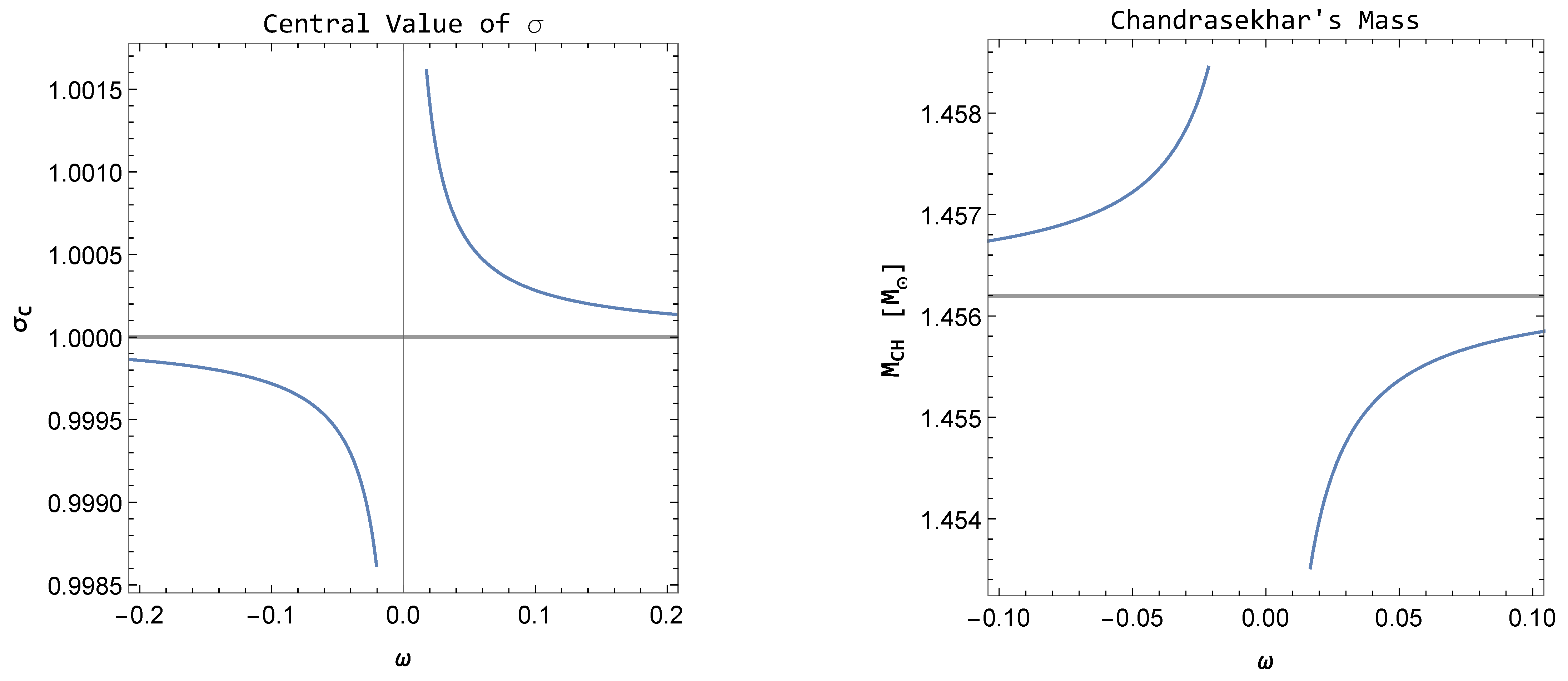
The results for this case are shown in Figure 1 and Figure 2. As expected, the theory with varying gravitational coupling is almost identical to the ordinary Newtonian one as the $\omega$ parameter value increases. For small and positive values of $\omega$, the central value of the $\sigma$ field starts to grow and, if it is interpreted as being proportional to the effective gravitational coupling $(G_{\mathrm{eff}}=G_0\sigma )$, this indicates a stronger gravity that lowers the star’s mass and radius. The situation for negative $\omega$ is the opposite. The central value of $\sigma$ starts to decrease, indicating a weaker gravity that increases the star’s mass and radius. Compared results for both positive and negative $\omega$ values are not symmetrical. We have checked that the solutions are more sensitive to negative values of the $\omega$ parameter.

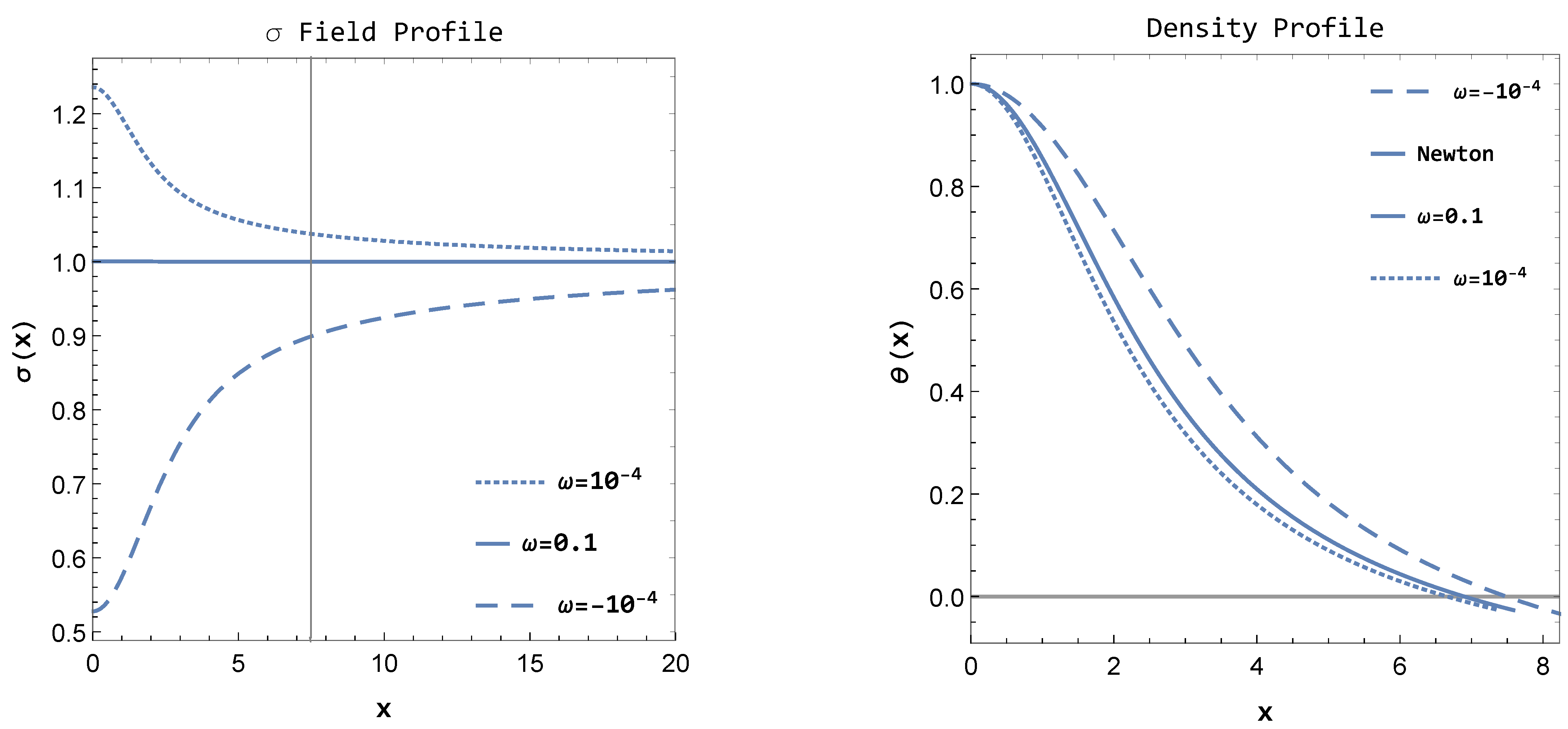
The sigma profile in Figure 2 indicates that, in the stellar exterior, the $\sigma$ field assume values $\sigma \ne 1$, and its derivative also does not vanish. This reminiscent feature of the extra scalar field $\sigma$ resembles the spontaneous scalarization effect, present in scalar-tensor theories. This consists in the development of a scalar cloud around the star [12,13]. Although the original spontaneous scalarization effect appears in the strong field regime of relativistic theories, there is remarkable similarity within the Newtonian context with the extra $\sigma$ field.

5. Final Remarks

Even though the actual description of the gravitational phenomena demands a covariant and relativistic formulation, the Newtonian gravity still works with acceptable accuracy for a broad range of astrophysical applications. The author of Ref. [10] proposed a non-relativistic version of a modified gravity theory inspired by the Brans–Dicke relativistic scalar-tensor theory of gravity. For simplicity, one can mention two new features of this theory: it possesses a new parameter $\omega$ and the strength of the effective gravitational coupling dictated by the field $\sigma$.

In this paper, this non-relativistic theory was applied to the structure of stellar configurations. While, in the exterior vacuum solutions, both $\psi$ and $\sigma$ satisfy the Laplace equation, with their behavior resembling the standard Newtonian potential, deviations are present in the interior solutions. Therefore, one cannot probe such new gravitational effects due to the existence of an intrinsic degeneracy with the equations of state for the stellar fluid. On the other hand, by fixing the equation of state, it is possible to measure the impact of the theory parameter $\omega$ on the astrophysical observables such as the star’s mass and the star’s radius.

The manifestation of the new gravitational features depends on the compactness of the star. Curiously, such dependence is not present in other modified gravity theories.

As the main result of the present study, the impact of the $\omega$ parameter on Chandrasekhar’s mass limit is discussed. If $\omega ={10}^{-4}$, then one finds $M_{\mathrm{CH}}=1.14M_{\odot }$, while, for $\omega ={10}^{-3}$, $M_{\mathrm{CH}}=1.41M_{\odot }$. Then, the existence of white dwarfs with masses around $1.3M_{\odot }$ [14,15] clearly rules out a $\omega$ value of order ${10}^{-4}$ or smaller. On the other hand, higher Chandrasekhar mass limits are allowed for negative $\omega$ values. This case would become very interesting in the event of a future detection of a white dwarf that is more massive than the currently accepted Chandrasekhar limit. Recent studies have pointed towards this possibility [16]. Finally, it is worth noting that modified gravity is not the only route to obtain modified Chandrashekhar mass limits, since they can also be obtained even within the Newtonian theory if, for example, the star is charged [17].

References

- Xue, C.; Liu, J.-P.; Li, Q.; Wu, J.-F.; Yang, S.-Q.; Liu, Q.; Shao, C.-G.; Tu, L.C.; Hu, Z.-K.; Luo, J. Precision measurement of the Newtonian gravitational constant. Natl. Sci. Rev. 2020, 7, 1803–1817. [Google Scholar] [CrossRef]
- Marra, V.; Perivolaropoulos, L. Rapid transition of Geff at zt≃0.01 as a possible solution of the hubble and growth tensions. Phys. Rev. D 2021, 104, L021303. [Google Scholar] [CrossRef]
- Brans, C.; Dicke, R.H. Mach’s principle and a relativistic theory of gravitation. Phys. Rev. 1961, 104, 925–935. [Google Scholar] [CrossRef]
- Dirac, P.A.M. The Cosmological constants. Nature 1937, 139, 323. [Google Scholar] [CrossRef]
- Dirac, P.A.M. New basis for cosmology. Proc. R. Soc. Lond. A 1938, A165, 199–208. [Google Scholar] [CrossRef] [Green Version]
- Horndeski, G.W. Second-order scalar-tensor field equations in a four-dimensional space. Int. J. Theor. Phys. 1974, 10, 363–384. [Google Scholar] [CrossRef]
- Landsberg, P.T.; Bishop, N.T. A principle of impotence allowing for Newtonian cosmologies with a time-dependent gravitational constant. Mon. Not. R. Astr. Soc. 1975, 171, 279–286. [Google Scholar] [CrossRef] [Green Version]
- McVittie, G.C. Newtonian cosmology with a time-varying constant of gravitation. Mon. Not. R. Astr. Soc. 1978, 183, 749–764. [Google Scholar] [CrossRef] [Green Version]
- Duval, C.; Gibbons, G.W.; Horvathy, P. Celestial mechanics, conformal structures and gravitational waves. Phys. Rev. D 1991, 43, 3907–3922. [Google Scholar] [CrossRef] [PubMed] [Green Version]
- Fabris, J.C.; Gomes, T.; Toniato, J.D.; Velten, H. Newtonian-like gravity with variable G. Eur. Phys. J. Plus 2021, 136, 143. [Google Scholar] [CrossRef]
- Kippenhahn, R.; Weigert, A.; Weiss, A. Stellar Structure and Evolution; Springer: Berlin/Heidelberg, Germany, 2012. [Google Scholar] [CrossRef]
- Damour, T.; Esposito-farese, G. Nonpertubative strong-field effects in tensor-scalar theories of gravitation. Phys. Rev. Lett. 1993, 70, 2–5. [Google Scholar] [CrossRef] [PubMed]
- Salgado, M.; Sudarsky, D.; Nucamendi, U. On spontaneous scalarization. Phys. Rev. D 1998, 58, 124003. [Google Scholar] [CrossRef] [Green Version]
- Kepler, S.O.; Kleinman, S.J.; Nitta, A.; Koester, D.; Castanheira, B.G.; Giovannini, O.; Costa, A.F.M.; Althaus, L. White dwarf mass distribution in the SDSS. Mon. Not. R. Astr. Soc. 2007, 375, 1315–1324. [Google Scholar] [CrossRef] [Green Version]
- Tang, S.; Bildsten, L.; Wolf, W.M.; Li, K.L.; Kong, A.K.H.; Cao, Y.; Cenko, S.B.; Cia, A.D.; Kasliwal, M.M.; Kulkarni, S.R.; et al. An accreting white dwarf near the Chandrasekhar limit in the Andromeda galaxy. Astrophys. J. 2014, 786, 61. [Google Scholar] [CrossRef] [Green Version]
- Pelisoli, I. A hot subdwarf–white dwarf super-Chandrasekhar candidate supernova Ia progenitor. Nat. Astron. 2021, 5, 1052–1061. [Google Scholar] [CrossRef]
- Liu, H.; Zhang, X.; Wen, D. One possible solution of peculiar type Ia supernovae explosions caused by a charged white dwarf. Phys. Rev. D 2014, 89, 104043. [Google Scholar] [CrossRef] [Green Version]
Figure 1.
Left: The behavior of the central value of the field. For positive , the gravitational coupling is larger than the Newtonian value, and, for negative , it is weaker. Right: The Chandrasekhar mass of such a limit star configuration. For positive , the mass is smaller than for negative values.
Figure 2.
Left: The field profile, with the approximate dimensionless radius of the star marked with the vertical thick line. For as small as , the gravitational coupling can be greater than the asymptotic Newtonian value. For negative small , the gravitational coupling at the star’s center is almost half the usual value. Right: The dimensionless density profile for the same values of . For values of of the order , the theory is practically indistinguishable from the Newtonian one.
Publisher’s Note: MDPI stays neutral with regard to jurisdictional claims in published maps and institutional affiliations. |
© 2021 by the authors. Licensee MDPI, Basel, Switzerland. This article is an open access article distributed under the terms and conditions of the Creative Commons Attribution (CC BY) license (https://creativecommons.org/licenses/by/4.0/).
Share and Cite
MDPI and ACS Style
Fabris, J.C.; Ottoni, T.; Toniato, J.D.; Velten, H. Stellar Structure in a Newtonian Theory with Variable G. Physics 2021, 3, 1123-1132. https://0-doi-org.brum.beds.ac.uk/10.3390/physics3040071
AMA Style
Fabris JC, Ottoni T, Toniato JD, Velten H. Stellar Structure in a Newtonian Theory with Variable G. Physics. 2021; 3(4):1123-1132. https://0-doi-org.brum.beds.ac.uk/10.3390/physics3040071
Chicago/Turabian StyleFabris, Júlio C., Túlio Ottoni, Júnior D. Toniato, and Hermano Velten. 2021. "Stellar Structure in a Newtonian Theory with Variable G" Physics 3, no. 4: 1123-1132. https://0-doi-org.brum.beds.ac.uk/10.3390/physics3040071