Article

Temperature-Compensated Spread Spectrum Sound-Based Local Positioning System for Greenhouse Operations

1
Graduate School of Agriculture, Kyoto University, Kyoto 6068502, Japan
2
Department of Ocean Mechanical Engineering, National Fisheries University, Shimonoseki 7596595, Japan
*
Author to whom correspondence should be addressed.
Submission received: 20 July 2020 / Revised: 15 August 2020 / Accepted: 22 September 2020 / Published: 27 September 2020

Abstract

:
A spread spectrum sound-based local positioning system (SSSLPS) has been developed for indoor agricultural robots by our research group. Such an SSSLPS has several advantages, including effective propagation, low cost, and ease of use. When using sound velocity for field position measurements in a greenhouse, spatial and temporal variations in temperature during the day can have a major effect on sound velocity and subsequent positioning accuracy. In this research, a temperature-compensated sound velocity positioning was proposed and evaluated in comparison to a conventional temperature sensor method. Results indicate that this new proposed method has a positioning accuracy to within 20 mm in a 3 m × 9 m ridged greenhouse. It has the potential to replace the current system of using the temperature sensors in a greenhouse.

1. Introduction

In recent years, agriculture has seen a sustained effort to improve the technology of field robotics [1,2]. These robots and new precision farming technologies are needed in places like Japan, where the population is ageing, and the supply of farm labor is declining [3]. However, few of these labor replacing robots have been designed and tested for greenhouse operations [4], though such automated robotic systems have the potential to aid farmers with the monitoring of crops, as well as for more efficient work operations in the greenhouse [5].
To automate agricultural systems, a new concept of Internet of Things (IoT) [6] that is based on building networks of devices and sensors has been developed. In many cases, these networks will require a localization system, which provides positioning information and controls the movement of the robots. To date, global navigation satellite systems (GNSS) [7,8], laser trackers [9], radio frequency identification (RFID) [10,11], Bluetooth low energy (BLE) beacon [12], ultrasound systems [13,14] and positioning by signal strength [15,16] have been utilized. However, these systems are not only limited to outdoor uses, but some them also have a low accuracy [17], are intolerant of obstacles, are very heavy and cannot be installed in a greenhouse [18]. To overcome these issues, we have developed a low-cost, high-accuracy and high noise-tolerant method based on a spread spectrum sound system [19]. The concept of using the spread spectrum sound (SSSound) enables indoor localization using only relatively inexpensive speakers and microphones. Such an SSSound system does not require a laser emitter, nor a photodetector to detect the pulse compared with a laser emitter system, and requires less devices compared to an RFID based system. In addition, it does not suffer from the disadvantages of a BLE bacon system, namely, low accuracy and interference with 2.4 GHz devices, etc.
The SSSound system determines position and provides localization inside a greenhouse based on the velocity of sound [20]. However, the speed of sound propagation is affected by the spatial variation of temperature within a greenhouse [21]. We hypothesize that position and a more representative mean sound velocity within the greenhouse can be simultaneously determined using a time of arrival (TOA) localization algorithm [22,23].
Moreover, the accuracy of this indoor spread spectrum sound localization system can be improved by directly calculating position and estimating sound velocity simultaneously based on a TOA algorithm [24]. Moreover, TOA localization does not require as many nodes to detect position as other localization algorithms.
In this research, the objective is to develop a new temperature compensation method using an estimated sound velocity algorithm embedded in the spread spectrum sound-based local positioning system. To do this, we first developed a spread spectrum sound system that can generate the SSSound signals. After that, the proposed temperature compensation method using a sound velocity estimation algorithm was compared with the conventional method of using temperature sensors. To evaluate field performance of the proposed estimation method, experiments were conducted in a small-sized greenhouse in summer and winter, when temperature variations are expected to be extreme. We also analyzed the positioning accuracy of the temperature compensation methods as well as the extent of temperature fluctuations within the greenhouse at these times.

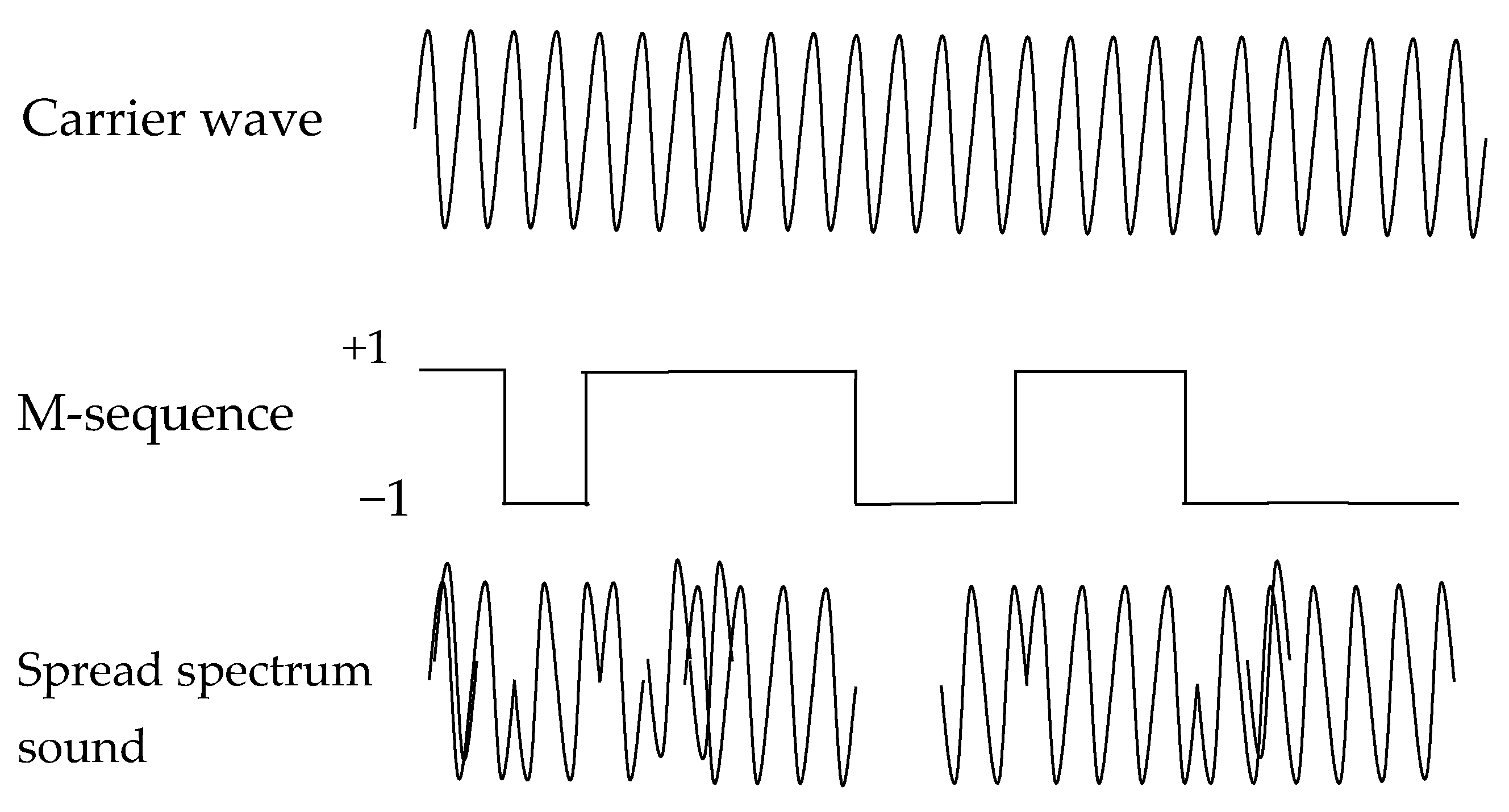
2. Spread Spectrum Sound Properties

Figure 1 illustrates the generation of the spread spectrum sound. The sound is encoded by maximal length sequence (M-sequence), which is a pseudo random sequence and has a good autocorrelation performance [25]. The length of the M-sequence was 1023, and the chip rate was 12 kcps. Then, it was multiplied by a carrier wave of 24 kHz. The frequency of the spread spectrum sound signal is from 12 to 36 kHz. The sampling frequency and sampling bit of the sound signals in the audio interface were 96 kHz and 16 bits, respectively.
At the start of the SSSound signal package, a trigger signal in an isolated channel is necessary to synchronize the start time of both transmission and reception. After the trigger signal was recognized, the cross-correlation [26] value was calculated based on the following Equation (1):
c ( t ) = n = 0 N 1 s ( n ) r ( n + t )
where N is the length of SSSound signal, t is the time of received data, s is transmitted signal, and r is received signal. The correlation values were then normalized by the average correlation value. After calculating the cross-correlation, the threshold Equation (2) was used to detect the signal peak. Figure 2 shows an obvious correlation value with a high peak, which corresponds to the arrival time of the sound signal.
C t h = C m a x + C a v e + 3 σ c o r r 2
where C m a x , C a v e , σ c o r r are the maximum value, average and standard deviation of cross-correlation value, respectively, and C t h is the threshold to detect the peak of signal arrival time. For calculating one SSSound signal set, the first 12,000 samples, that is, half of the total 24,000 samples, were used to calculate the cross-correlation. This because the scale of the greenhouse was small, and the expected time for signal propagation should occur within the first half of the total samples. The example in Figure 2 shows the normalized samples of the received signals, which had a threshold value of 0.95, and identifies the correct peak at the 1330th signal and the reflected peak at 1600th signal.
The sound velocity parameter in Equation (3) is sensitive to temperature; thus, the conventional means to compensate for this is using a precise temperature measurement (sensor) taken at speaker i to obtain the T s i to calculate the distance d i from the speaker i to the microphone target by the following Equation (4):
v i = 331.5 + 0.61 ( T s i )
d i = ( v i ) ( t i )
where T s i is the temperature at speaker i, v i is the speed of sound signals (m/s) and t i is the propagation time of emitted sound from the i th node in an inverse GPS-like system, which refers to the target passively receiving the navigation signal [27]. Finally, three known distances are needed to obtain a position using trilateration in the conventional method.
The proposed method using an estimated sound velocity for calculating the position and the sound velocity is based on a TOA localization algorithm. Equation (5) indicates the relationship between distances and coordinates of each node and measurement position simultaneously. This differs from the conventional method (Equation (4)), which uses data from temperature sensors [28].
( t i ) ( v e ) = ( x s x i ) 2 + ( y s y i ) 2 + ( z s z i ) 2 f i ( x s ,   y s ,   z s , v e ) = ( x s 0 x i ) 2 + ( y s 0 y i ) 2 + ( z s 0 z i ) 2 ( t i ) ( v e )
where, t i is propagation time of emitted sound of the i th node, ( x s ,   y s ,   z s ) is the estimated position of the target, ( x i ,   y i ,   z i ) is the position of the i th node, and ( v e ) is the estimated sound velocity. It is assumed in Equation (5) that the sound velocity of the propagated sound between the transmitters and receiver in the greenhouse is constant.
The unknowns are the position coordinates ( x s ,   y s ,   z s ) and the estimated sound velocity ( v e ) . When the transmitting time ( t i ) is measured, the positions of the nodes are known and the provisional sound velocity can be set. Therefore, the four unknowns ( x s ,   y s ,   z s ) and ( v e ) can be estimated when the number of nodes is larger than four, since at least a system of four equations in Equation (5) are needed in order to solve the four unknowns. The function, f i ( x s ,   y s ,   z s , v e ) , represents the positioning error, which indicates the distance of the target position minus the sound propagation distance.
This is difficult to compute because Equation (5) is a non-linear equation. Thus, it needs to be linearized by a Taylor expansion, ( x s ,   y s ,   z s ) and ( v e ) estimated by sequential computation of the function f i ( x s ,   y s ,   z s , v e ) , which is also defined in Equation (5). f i ( x s ,   y s ,   z s , v e ) is linearized by the first-order Taylor-series expansion at x s 0 ,   y s 0 ,   z s 0 ,   v e 0 , as in Equation (6).
f i ( x s ,   y s ,   z s , v e ) = ( x s 0 x i ) 2 + ( y s 0 y i ) 2 + ( z s 0 z i ) 2 ( t i ) v e 0 + f i x s ( x s x s 0 ) + f i y s ( y s y s 0 ) + f i z s ( z s z s 0 ) + f i v e ( v e v e 0 )
The defined matrixes and vectors are as in Equation (7)
Δ d i = f i x s Δ x s + f i y s Δ y s + f i z s Δ z s + f i v e Δ v e Δ x s = ( x s x s 0 ) Δ y s = ( y s y s 0 ) Δ z s = ( z s z s 0 ) Δ v e = ( v e v e 0 ) Δ d = [ Δ d 2 Δ d 3 ]           A = [ f 2 x s f 2 y s f 2 z s f 3 x s f 3 y s f 3 z s     f 2 v e f 3 v e ] Δ x = [ Δ x s Δ y s     Δ z s Δ v e ] T Δ d = A Δ x
A is the observation matrix. The generalized inverse matrix of A is multiplied on both sides of the Equation (8). An iterative least squares method is used by iterating 50 times when ∆x is approaching 0 and gives the approximate coordinate of the target.
Δ x = ( A T A ) 1 A T Δ d

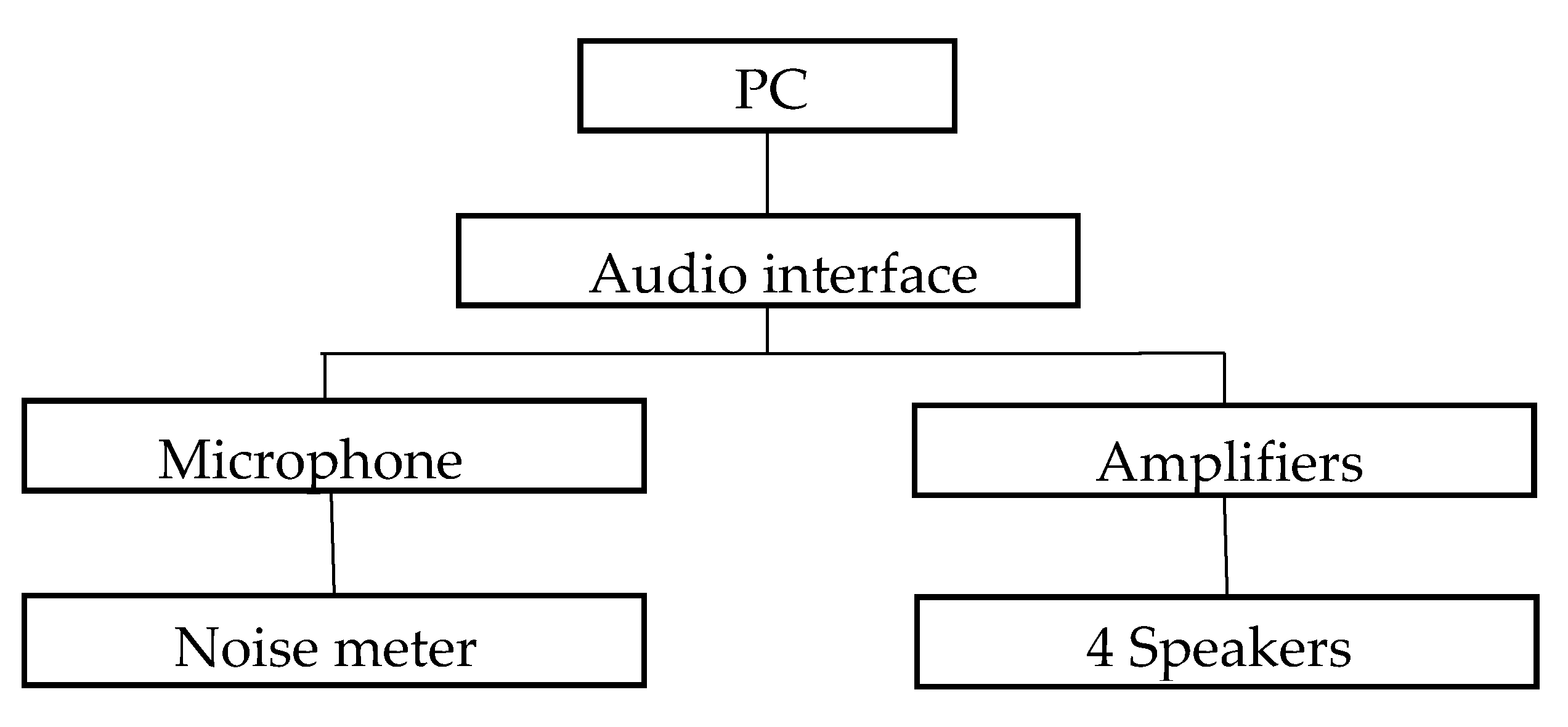
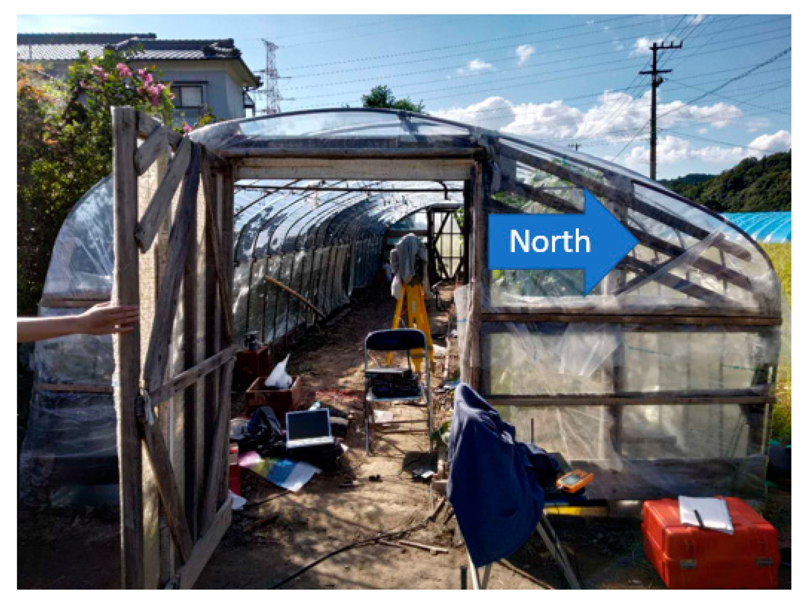
3. Materials and Methods
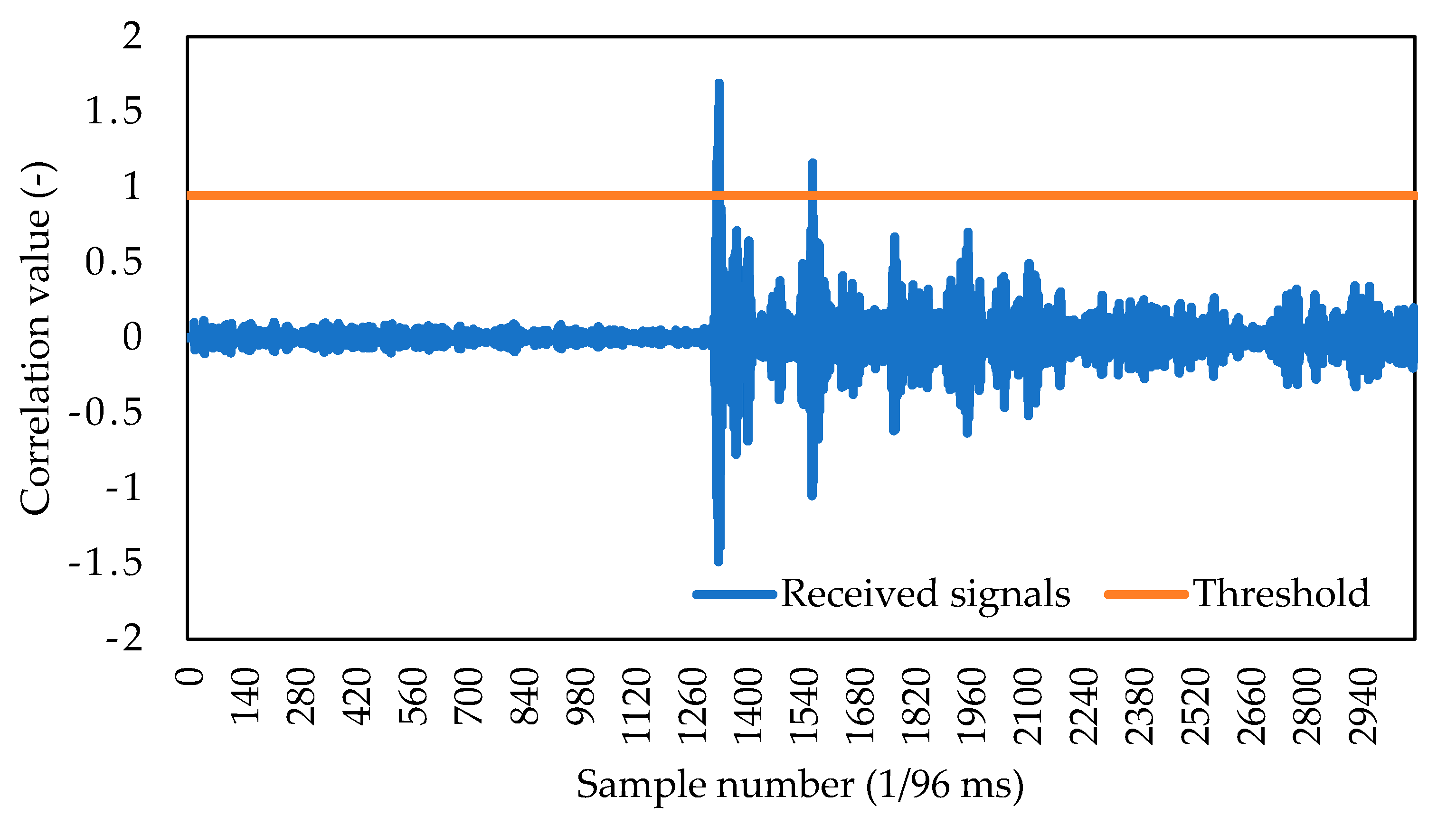
A ridged greenhouse without plants to interfere with the path of the sound signal was used as the target localization area with doors shut, no ventilation open, or wind inside for the experiment. For this small-sized greenhouse, a set of four speakers and a microphone are adequate. Temperature variations within the greenhouse can have a major effect on the sound-based system since the greenhouse covering was made from common polyethylene plastic, which enables radiation heating.
The spread spectrum sound signals were generated by a laptop computer (PC), converted from digital to analog signals at the audio interface (Roland OCTA-CAPTURE UA-1010, Hamamatsu, Japan), amplified by amplifiers (Kama Bay Amp Rev. B, Scythe Inc., Ontario, CA, USA) and emitted by four twitters, which are high-frequency speakers (FT28D, Fostex Company, Tokyo, Japan). Before the experiment, the sound level was calibrated at 80 dB using a noise meter (LA-4440, Ono Sokki, Yokohama, Japan). Then, emitted sound was received by a microphone (M30, Earthworks, Milford, CT, USA) and converted from analog to digital signals at the audio interface, and the position coordinates were calculated at the PC. The computer processed the correlation calculation of the received sound signals, acquiring a correlation peak to obtain the received time of spread spectrum sound and the position estimation. The M-sequence’s period was 1023, with is also combined with the time division multiple access (TDMA) method. Figure 3 shows outline of the localization system.
The experiment was conducted in a typical farmer’s small greenhouse (width 3.5 m × length 13 m × height 2 m) in Toon-shi of Ehime prefecture, Japan. The experimental greenhouse was recovered with new polyethylene film before the experiment in order to fit the condition for controlling for air ventilation. Figure 4 shows the front door, as well as the orientation of the greenhouse after recovery, and Figure 5a shows the four speakers, the total station at the edges for reference coordinates and the overall setup of the experiment, which was conducted on a sunny summer day with local temperature ranging from 20 to 34 °C (27 September 2018). There was some drizzle in the morning. Figure 5b shows the experiment conditions where some radish plants were growing in the greenhouse on a cloudy winter day, and where temperatures ranged from 0 to 10 °C (23 January 2019).
Figure 6 illustrates the experimental localization area, as well as the settings of the speakers and microphone. The whole experiment was conducted in a closed greenhouse with the greenhouse doors shut most of the time during the two days of the experiment. There were no people inside the greenhouse during the measurements. The experiment started from 10:00 to 19:00 with temperatures recorded hourly (a total of 10 measurements) and SSSound data recorded at least 6 times at each sampling. Recorded temperatures ranged from 4 to 38 °C, the typical range found in greenhouse farming situations. The outside temperature ranged from 0 to 27 °C. It is believed that the temperature data obtained cover typical greenhouse temperatures in winter as well as in summer, and is representative of the potential influences of temperature variation on the spread spectrum sound localization system.
Figure 7 shows the setup of the four speakers with their accompanying temperature sensors (located at (0,3), (9,3), (9,0) and (0,0) for speakers 1 to 4, respectively). There were some kiwi fruit plants outside the greenhouse creating some shades covering the area where speakers 1 and 2 were. The recorded temperatures are expected to be lower than those at speakers 3 and 4.
Figure 8 shows the horizontal view of the experimental setting, showing that the speaker and measurement positions (50 cm above the ground) were higher than the ridges. Since all the nodes were set at a 50 cm height above ground, the calculated target position was determined in 2-dimensional coordinates. Figure 9 illustrates the actual experiment conditions with the temperature sensor covered by a wind tube (Figure 9a) and the microphone fixed at a height of 50 cm (Figure 9b). A fan inside the wind tube was switched on to increase equilibration with the surrounding air temperature. The tube was placed a few centimeters below the speakers.

4. Results

4.1. Evaluation of the Temperature in the Greenhouse

Temperature differed at each speaker within the greenhouse (0.5 m above ground). Moreover, the speakers (1 and 2) in shaded areas had lower temperatures due to the received radiation energy being reduced. Figure 10 shows the results of greenhouse temperature data at the four speakers during a typical summer season (the upper four curves) and winter season (the lower four curves), which represents a temperature range from 2 °C in winter up to 35 °C in summer. It was observed that the maximum temperature differential can be up to 11 °C when the sun rays are at their strongest (14:00 in winter). However, after sunset in summer (17:00) and in winter (16:00), temperatures dropped, making any temperature differences in the greenhouse negligible. A microclimate phenomenon, that is, small areas with differing atmospheric conditions [29], occurred during the day and created approximately 6 °C differences within the greenhouse. A convective heat transfer was observed as the warm moist air rose to the top and condensed on the walls of the greenhouse. Such condensation would not happen if there was air flow or ventilation in the greenhouse [30]. The temperature distribution during the daytime was more uniform in the summer than the winter [31] and created horizontal regions of temperature differences in the greenhouse. During the summer, experiment recordings were paused temporarily at 12:15 to open the greenhouse door for 30 min to reduce overheating in the greenhouse. Thus, there was a temperature drop at 13:00 in the summer of approximately 5 °C.

4.2. Comparison of the Conventional Temperature Sensor Method and the Estimated Sound Velocity Method

Figure 11 shows the average position error of the conventional temperature sensor method (sensor method) and estimated sound velocity method (estimated method) in summer. The sensor method uses temperature sensor data to calculate the sound velocity and then calculates the position results, whilst the estimated method uses the estimated sound velocity to calculate the position results directly. The average position error for the sensor method was 23.12 mm, while for the estimated method it had only a 11.14 mm error. In Figure 11, the largest temperature differences occurred at 15:00. This is consistent with the sensor method generating a large positioning error when the temperature differences within the greenhouse were large. The sensor method was more accurate at 17:00 when the temperature difference between the speakers was minimal. At this time, both methods had position errors of around 20 mm. The estimated method was not as accurate at 12:00, as well as at 16:00, as other times between dawn and dusk (Figure 11). These two periods correspond to times when there were rapid changes in temperature within the greenhouse, consistent with temperature variations (at different speakers) adversely affecting sound velocity estimates within the greenhouse. Temperature sensors merely measure and record the temperature near the sensor (speaker); thus, they do not accurately reflect the temperature over the whole sound propagation pathway.
Similarly, Figure 12 shows that the average position error in winter was 38.94 mm using the sensor method, while the average error was 17.17 mm using the estimated method. Compared to the summer results, the winter temperature differences in the greenhouse propagated larger positioning errors for the sensor method than for the estimated method throughout the whole day. In winter, when the outside is lower than that inside the greenhouse, larger temperature variations within the greenhouse can be generated with fluctuating sunlight radiation levels. Moreover, water vapor lost (transpiration) from the leaves of the radish plants’ may also have affected sound velocities in the winter experiment, giving rise to larger position errors in winter compared to summer for both temperature compensation methods.
Figure 13 shows the relationship between position error and temperature differences in the greenhouse for both the summer and winter experiments. Position errors can be generated by errors in sound velocity estimates due to temperature variations along the signal transmission path. The standard deviation of temperature used in Figure 13 was calculated from the four temperature sensors placed at each of the speakers during the experiment. Temperature differences in the greenhouse in winter, as measured by the sensor method, were larger than those observed in the summer experiment (Figure 11), as were the observed positioning errors. As the desired precision was set to a minimum of 20 mm in a previous study [22], the estimated method achieved results that were more stable and closer to the desired precision than those achieved by the sensor method.
Though the estimated sound velocity method assumes that sound velocity is uniformly distributed, the result shows that it can tolerate uneven sound velocity generated by large temperature differences within a small-sized greenhouse. The results demonstrate that the estimated method better reflects actual sound velocities within the greenhouse, and thus provides more accurate positioning results than the sensor method (position errors at or below the 20 mm limit). The proposed algorithm better approximates the average sound velocity along the whole signal transmission path than the conventional calculation.

5. Discussion

In this research a new method for estimating average temperature along the propagated sound path is used to estimate average sound velocity between the transmitter and receivers. When temperatures varied substantially within the greenhouse, this average temperature estimation method was more accurate at deriving sound velocity than the conventional sensor method, which uses local temperature sensor measurements at each node.
To evaluate the accuracy of this new temperature compensation method embedded in an SSSLPS system, positioning measurements were undertaken both in summer and winter when seasonal variations in temperature within the greenhouse are expected to be at their largest. Temperature variations of up to 11 °C were observed in winter, while variations less than 6 °C were observed in summer, resulting in differences in positioning accuracy of around 5–10 mm between the two seasons. The low outside temperature in winter created large fluctuations in the daytime temperature within the greenhouse, whilst we speculated that the transpiration from the radish plants’ growing there at the time also affected surrounding air temperature and humidity variation within the greenhouse [32]. Microclimatic temperature layers inside the greenhouse [29], especially in winter, effectively trap hot air and generate convection phenomenon with the surrounding cold air.
To evaluate and compare the positioning accuracy of the estimated versus the conventional sensor method, average positioning performance was measured, with the estimated method achieving a better position accuracy than the desired precision of less than 20 mm. The overall positioning accuracy of the estimated method (14 mm) was higher than the sensor method (30 mm) for the combined summer and winter results. The estimated method has the advantage of simultaneously calculating position and estimating sound velocity compared to the sensor method, but the calculation is more complicated and requires more nodes. Positioning errors can also be affected by the signal time of arrival measurement errors, as well as the setting error associated with total station measurement errors, etc.
Future research should include using more temperature sensors as nodes, increasing the size of the greenhouse to that found in large commercial operations, developing a hybrid system with inertial measurement units (IMU), as well as improving the noise tolerance of the system, etc. It is believed that a spread spectrum sound localization system can be used in the presence of operating drones, as well as other challenging environments.

6. Conclusions

This research proposed a new temperature compensation method that can be used with localization systems that estimate position using sound for accurate positioning inside small-sized greenhouses. The summer and winter experimental result demonstrate that the newly developed temperature compensation method does not require the setup of temperature sensors, while providing similar or even better positioning accuracy than compensation based on conventional temperature sensor measurements. The estimate algorithm works well in a small controlled indoor environment and can predict the average sound velocity along the propagated path between the transmitters and receiver. This also means that the proposed estimated method can compensate for temperature-generated errors in an SSSLPS used in the small-sized greenhouse.
This new temperature compensation method achieved a positioning error using SSSLPS at or below 20 mm during the season, even at extremes in summer and winter. This accuracy can outperform most of the existing positioning systems and can be used to control multiple robots, such as ground vehicles, in a greenhouse. By simultaneously calculating the position and estimating the average sound velocity, more convenient temperature compensation in a greenhouse is achieved without the need to use temperature sensors. It should be noted that both calculations are based on a TOA algorithm. It is believed that the SSSLPS can contribute greatly to the development of IoT in agriculture and indoor precision agriculture.

Author Contributions

Conceptualization, L.W.J.T. and T.S. (Tomoo Shiigi); data curation, T.S. (Tomoo Shiigi) and X.Z.; formal analysis, L.W.J.T.; funding acquisition, N.K.; methodology, L.W.J.T. and T.S. (Tomoo Shiigi); project administration, T.S. (Tomoo Shiigi) and T.S. (Tetsuhito Suzuki); resources, N.K.; software, Z.H.; supervision, N.K.; validation, L.W.J.T.; visualization, L.W.J.T. and Z.H.; writing—original draft, L.W.J.T.; writing—review and editing, T.S. (Tomoo Shiigi), Z.H., X.Z., T.S. (Tetsuhito Suzuki) and Y.O. All authors have read and agreed to the published version of the manuscript.

Funding

This research was funded by JSPS KAKENHI, grant number 18H05364.

Acknowledgments

I would like to gratefully acknowledge the support of Garry John PILLER from Kyoto University for proof-reading the manuscript.

Conflicts of Interest

The authors declare no conflict of interest.

References

  1. Vougioukas, S.G. Agricultural robotics. Annu. Rev. Control. Robot. Auton. Syst. 2019, 2, 365–392. [Google Scholar] [CrossRef]
  2. Bechar, A.; Vigneault, C. Agricultural robots for field operations. Part 2: Operations and systems. Biosyst. Eng. 2017, 153, 110–128. [Google Scholar] [CrossRef]
  3. Hayashi, S.; Yamamoto, S.; Saito, S.; Ochiai, Y.; Kamata, J.; Kurita, M.; Yamamoto, K. Field Operation of a Movable Strawberry-harvesting Robot using a Travel Platform. JARQ 2014, 48, 307–316. [Google Scholar] [CrossRef] [Green Version]
  4. Mautz, R. Overview of current indoor positioning systems. Geod. Cartogr. 2009, 35, 18–22. [Google Scholar] [CrossRef]
  5. Kawamura, N.; Namikawa, K.; Fujimura, T.; Ura, M. Study on Agricultural Robot (Part 1). J. Jpn. Soc. Agric. Mach. 1984, 46, 353–358. [Google Scholar] [CrossRef]
  6. Spachos, P. Towards a low-cost precision viticulture system using internet of things devices. IoT 2020, 1, 2. [Google Scholar] [CrossRef] [Green Version]
  7. Koura, Y.; Suzuki, H.; Ogawa, K.; Kamei, Y.; Nakamura, M. GPS COMPASS: A low cost gps direction sensor of two antenna type. In Proceedings of the 14th International Technical Meeting of the Satellite Division of The Institute of Navigation (ION GPS 2001), Salt Lake City, UT, USA, 11–14 September 2001; pp. 2700–2707. [Google Scholar]
  8. Mercado, D.A.; Flores, G.; Castillo, P.; Escareno, J.; Lozano, R. GPS/INS/optic flow data fusion for position and velocity estimation. In Proceedings of the 2013 International Conference on Unmanned Aircraft Systems (ICUAS), Atlanta, GA, USA, 28–31 May 2013; pp. 486–491. [Google Scholar]
  9. Jia, L.; Xue, B.; Chen, S.; Wu, H.; Yang, X.; Zhai, J.; Zeng, Z. A high-resolution ultrasonic ranging system using laser sensing and a cross-correlation method. Appl. Sci. 2019, 9, 1483. [Google Scholar] [CrossRef] [Green Version]
  10. Yan, H.; Chu, J. RFID positioning algorithm based on BA optimization. In Proceedings of the 2020 5th International Conference on Computer and Communication Systems (ICCCS), Shanghai, China, 22–24 February 2020; pp. 854–858. [Google Scholar]
  11. Shirehjini, A.A.N.; Yassine, A.; Shirmohammadi, S. An RFID-based position and orientation measurement system for mobile objects in intelligent environments. IEEE Trans. Instrum. Meas. 2012, 61, 1664–1675. [Google Scholar] [CrossRef]
  12. Spachos, P.; Papapanagiotou, I.; Plataniotis, K.N. Microlocation for smart buildings in the era of the internet of things: A survey of technologies, techniques, and approaches. IEEE Signal Process. Mag. 2018, 35, 140–152. [Google Scholar] [CrossRef]
  13. Atri Mandal, C.V.L. Beep: 3D indoor positioning using audible sound. In Proceedings of the Second IEEE Consumer Communications and Networking Conference, Las Vegas, NV, USA, 3–6 January 2005; pp. 348–353. [Google Scholar]
  14. Khyam, M.d.O.; Ge, S.S.; Li, X.; Pickering, M.R. Highly accurate time-of-flight measurement technique based on phase-correlation for ultrasonic ranging. IEEE Sens. J. 2017, 17, 434–443. [Google Scholar] [CrossRef]
  15. Huang, Z.; Tsay, L.W.J.; Shiigi, T.; Zhao, X.; Nakanishi, H.; Suzuki, T.; Ogawa, Y.; Kondo, N. A noise tolerant spread spectrum sound-based local positioning system for operating a quadcopter in a greenhouse. Sensors 2020, 20, 1981. [Google Scholar] [CrossRef] [PubMed] [Green Version]
  16. Chan, E.C.L.; Baciu, G.; Mak, S.C. Using Wi-Fi signal strength to localize in wireless sensor networks. In Proceedings of the 2009 WRI International Conference on Communications and Mobile Computing, Kunming, China, 6–8 January 2009; pp. 538–542. [Google Scholar]
  17. Bellone, T.; Dabove, P.; Manzino, A.M.; Taglioretti, C. Real-time monitoring for fast deformations using GNSS low-cost receivers. Geomat. Nat. Hazards Risk 2016, 7, 458–470. [Google Scholar] [CrossRef]
  18. De Preter, A.; Anthonis, J.; De Baerdemaeker, J. Development of a robot for harvesting strawberries. IFAC Pap. 2018, 51, 14–19. [Google Scholar] [CrossRef]
  19. Huang, Z.; Wai Jacky, T.L.; Zhao, X.; Shiigi, T.; Nakanishi, H.; Suzuki, T.; Naoshi, K. Noise Tolerance evaluation of spread spectrum sound-based positioning system for a quadcopter in a greenhouse. IFAC Pap. 2019, 52, 239–242. [Google Scholar] [CrossRef]
  20. Osada, Y.; Fujimoto, H.; Miura, S.; Sweeney, A.; Kanazawa, T.; Nakao, S.; Sakai, S.; Hildebrand, J.A.; Chadwell, C.D. Estimation and correction for the effect of sound velocity variation on GPS/Acoustic seafloor positioning: An experiment off Hawaii Island. Earth Planets Space 2003, 55, e17–e20. [Google Scholar] [CrossRef] [Green Version]
  21. Wenzhou, S. Analysis of the influence about uncertain sound velocity on the positioning of seafloor control points. OFOAJ 2019, 9. [Google Scholar] [CrossRef]
  22. Widodo, S.; Shiigi, T.; Hayashi, N.; Kikuchi, H.; Yanagida, K.; Nakatsuchi, Y.; Ogawa, Y.; Kondo, N. Moving object localization using sound-based positioning system with doppler shift compensation. Robotics 2013, 2, 36–53. [Google Scholar] [CrossRef] [Green Version]
  23. Ni, D.; Postolache, O.A.; Mi, C.; Zhong, M.; Wang, Y. UWB indoor positioning application based on kalman filter and 3-D TOA localization algorithm. In Proceedings of the 2019 11th International Symposium on Advanced Topics in Electrical Engineering (ATEE), Bucharest, Romania, 28–30 March 2019; pp. 1–6. [Google Scholar]
  24. Le, T.-K.; Ono, N. Numerical formulae for TOA-based microphone and source localization. In Proceedings of the 2014 14th International Workshop on Acoustic Signal Enhancement (IWAENC), Juan-les-Pins, France, 8–11 September 2014; pp. 178–182. [Google Scholar]
  25. Mostafa, M.H.; Chamaani, S.; Sachs, J. Singular spectrum analysis-based algorithm for vitality monitoring using M-sequence UWB sensor. IEEE Sens. J. 2020, 20, 4787–4802. [Google Scholar] [CrossRef]
  26. Huang, L.; Zhang, S.; Wang, J.; Zhang, X. Classification of improved cross-correlation function to determine speaker location from microphone array. In Proceedings of the 2019 IEEE Fifth International Conference on Big Data Computing Service and Applications (BigDataService), Newark, CA, USA, 4–9 April 2019; pp. 209–214. [Google Scholar]
  27. Matano, T.; Tanaka, T. Inverse-GPS positioning using carrier phase. IEEJ Trans. EIS 2003, 123, 255–261. [Google Scholar] [CrossRef] [Green Version]
  28. Le, T.-K.; Ono, N. Reference-distance estimation approach for TDOA-based source and sensor localization. In Proceedings of the 2015 IEEE International Conference on Acoustics, Speech and Signal Processing (ICASSP), South Brisbane, Australia, 19–24 April 2015; pp. 2549–2553. [Google Scholar]
  29. Li, G.; Tang, L.; Zhang, X.; Dong, J.; Xiao, M. Factors affecting greenhouse microclimate and its regulating techniques: A review. IOP Conf. Ser. Earth Environ. Sci. 2018, 167, 012019. [Google Scholar] [CrossRef]
  30. Kumar, M. Experimental study on natural convection greenhouse drying of papad. J. Energy South. Afr. 2017, 24, 37–43. [Google Scholar] [CrossRef]
  31. Perret, J.S.; Al-Ismaili, A.M.; Sablani, S.S. Humidification-dehumidification system in a greenhouse for sustainable crop production. In Proceedings of the Ninth International Water Technology Conference, Sharm El-Sheikh, Egypt, 17–20 March 2005; pp. 849–862. [Google Scholar]
  32. Yang, X.; Short, T.H.; Fox, R.D.; Bauerle, W.L. Transpiration, leaf temperature and stomatal resistance of a greenhouse cucumber crop. Agric. For. Meteorol. 1990, 51, 197–209. [Google Scholar] [CrossRef]
Figure 1. Generation of spread spectrum sound from carrier wave and M-sequence.
Iot 01 00010 g001
Figure 2. Normalized correlation value and threshold for peak detection from received signals.
Iot 01 00010 g002
Figure 3. Devices connection of the localization system.
Iot 01 00010 g003
Figure 4. Front of the greenhouse and the north direction.
Iot 01 00010 g004
Figure 5. (a) Speakers and microphone setting in the greenhouse in summer; (b) similar settings in winter whilst there were some radish plants in the field.
Iot 01 00010 g005
Figure 6. Speakers and microphone position and the size of measurement field.
Iot 01 00010 g006
Figure 7. Measurement area, position of nodes and the four temperature sensors in a 2-dimensional plane.
Iot 01 00010 g007
Figure 8. Horizontal view of the speaker and microphone.
Iot 01 00010 g008
Figure 9. (a) Temperature sensor with a wind tube placed near the speaker at 50 cm; (b) microphone at the center of the greenhouse, 50 cm aboveground.
Iot 01 00010 g009
Figure 10. Temperatures of speakers in greenhouse.
Iot 01 00010 g010
Figure 11. Position error of the sensor and estimated methods in summer.
Iot 01 00010 g011
Figure 12. Position error of the sensor and estimated methods in winter.
Iot 01 00010 g012
Figure 13. Relationship between position error of the two methods and temperature standard deviation.
Iot 01 00010 g013

