Estimators for Time Synchronization—Survey, Analysis, and Outlook


1
Institute of Applied Microelectronics and CE, University of Rostock, 18119 Rostock , Germany
2
Department of Computer Science, University of Rostock, 18059 Rostock, Germany
*
Author to whom correspondence should be addressed.
IoT 2020, 1(2), 398-435; https://0-doi-org.brum.beds.ac.uk/10.3390/iot1020023
Submission received: 8 October 2020
/
Revised: 11 November 2020
/
Accepted: 14 November 2020
/
Published: 17 November 2020
Abstract
:Time (or clock) synchronization is a large and vital field of research, as synchronization is a precondition for many applications. A few example applications are distributed data acquisition, distributed databases, and real-time communication. First, this survey paper introduces the research area of time synchronization and emphasizes its relation to other research areas. Second, we give an overview of the state-of-the-art of time synchronization. Herein, we discuss both established protocol and research approaches. We analyze all techniques according to three criteria: used estimation algorithm, achievable synchronization accuracy, and the experimental conditions. In our opinion, this analysis highlights potential improvements. The most important question in this survey is as follows: which estimation method can be used to achieve which accuracies under which conditions? The intention behind this is to identify estimation methods that are particularly worth considering, as these already achieve good results in the wireless area but have not yet been examined in the wired area (and vice versa). This survey paper differs from other surveys in particular through the consideration of wireless and wired synchronization and the focus on estimation algorithms and their achievable accuracy.
1. Introduction
1.1. Motivation
There are many applications of time synchronization in the IoT (Internet of Things) and IIoT (Industrial Internet of Things). In a smart factory, the production robots which work together on a production line must be synchronized precisely. Exact time synchronization is also important when multiple motors move one mechanical load [1,2] or, in general, when drives work together [3]. In a smart power plant or in the area of energy supply, time synchronization is of decisive importance both for the analysis of blackouts and for controlling the stability of the power grid [4].
In addition, time synchronization is essential for communication based on TDMA (Time Division Multiple Access). TDMA is used, e.g., in real-time networks. Each device is given an exclusive transmission time slot. Compliance with these time slots prevents collisions. The better the devices are synchronized, the more precisely the time slots can be adhered. Consequently, the available bandwidth can be utilized better [5]. However, if the devices are inaccurately synchronized, slack times must be inserted to guarantee that only one device is transmitting at a specific point in time. This leads to unused bandwidth. TDMA methods are used in practice in many real-time Ethernet protocols such as Ethernet Powerlink or SERCOS III. Furthermore, wireless real-time communication is typically based on TDMA [6]. In addition to real-time networks, TMDA is also used in WSNs (Wireless Sensor Networks). Here, the sensor nodes communicate, e.g., only for a short time period and otherwise remain in a sleep mode to save energy [7,8].
Another application of time synchronization is distributed data acquisition. An example is the nuclear fusion experiment W7-X (Wendelstein 7-X). The W7-X experiment has a relatively large spatial expansion as the diameter of the vacuum vessel is approximately 16 meters. Above all, it is a highly dynamic system (magnetically enclosed plasma). Both the control of the system and the scientific evaluation of the experiments require measurement timestamps with accuracies in the range of nanoseconds [9]. Measured parameters are, e.g., temperature, electron density, and plasma properties [10]. These requirements also apply to similar large-scale experiments such as the particle accelerators at CERN (European Organization for Nuclear Research) [11]. Another example of distributed data acquisition as an application of time synchronization is the interconnection of several radio telescopes in order to achieve a significantly higher resolution. If several such telescopes are distributed over different continents, the data needs to be timestamped precisely in order to be fused in postprocessing. With this method, the Event Horizon Telescope could for the first time take a picture of the direct vicinity of a black hole [12]. Another example is the observation of the stability of bridges, stadiums, and high-rise buildings using wireless sensors. Here, a synchronization accuracy of at least 120 s is required to enable detecting vibrations [13].
In general, time synchronization enables ensuring the sequence of events [5]. Therefore, it is also essential for the financial world and online trading as the sequence of transactions is particularly important here [5]. Time synchronization is also important for distributed databases to ensure consistency as well as to optimize throughput and latency [5].
1.2. Problem Definition and Objectives of the Survey Paper
Typically, slave devices are synchronized to a master or reference time. However, there are also completely distributed approaches, especially for WSNs, in which all devices find a common time base.
The aim of this survey paper is to discuss algorithmic procedures for precise time synchronization. The aim is to give an overview, to classify the research domain, and to present the current state-of-the-art. When analyzing the state-of-the-art in this article in contrast to other works, the focus is particularly on estimation algorithms to determine future research needs.
The major challenges of time synchronization are that clock generators and communication channels are not ideal in reality. This leads to inaccuracies that need to be compensated. For clock generators, quantization, frequency changes (e.g., due to temperature effects [5,14]), random variations with every tick (jitter), random frequency change (wander), and aging effects (over long periods of time) are to be expected. For communication channels, variations in the network delay (e.g., due to switching queues) and variable processing times are particularly problematic, especially for software (SW) processing. The following requirements for a time synchronization approach can be defined:
- Accuracy: The remaining time difference between master and slave, which cannot be compensated by synchronization, should be as small as possible. In this context, there are two parameters defined. The offset is the time difference between master and slave. Compensating the offset is referred to as synchronization. The skew is the frequency difference between both. Compensating the skew is referred to as syntonization.
- Scalability and bandwidth efficiency: Synchronization messages always generate an overhead. If less bandwidth is used for synchronization, more bandwidth is available for the actual tasks of the distributed system (control, data acquisition, data exchange, etc.). This is crucial for the scalability of an synchronization approach, as the synchronization of all devices might be impossible at some point due to limited bandwidth and thousands of devices to be synchronized. Additionally, reducing the number of messages also reduces the energy consumption. This is especially important in wireless scenarios with battery-powered devices (note that communication typically requires a lot more energy than computing [15]).
- Computational efficiency: The time synchronization requires additional computing power on devices. The less additional computing power is required for synchronization, the more is available for the actual tasks of the devices.
- Hardware (HW) requirements: The HW requirements are also decisive. This applies to both the end devices (e.g., networks interface cards) and the network infrastructure (e.g., switches). Lower HW requirements lead to lower installation costs and greater future-proofness.
- Robustness: Depending on the use case, it might be important that an approach is especially robust. Robustness is very relevant in highly dynamic IoT scenarios (high node churn and frequent topology changes). In IIoT scenarios, robustness against failing nodes and links is important in order to achieve high availability of the system.
- Security: One major concern in modern networks is security. Consequently, it is also relevant for synchronization. Especially, in IIoT scenarios, it is crucial that secure time synchronization protocols are safe against malicious nodes and attacks, as a failing synchronization can lead to failure of the entire system.
The individual requirements must always be weighed against each other. For example, the accuracy of WSN approaches is of less importance than the energy efficiency [8]. In contrast, in wired real-time networks, high energy requirements and special HW are sometimes accepted in order to achieve a high level of accuracy [9,11].
1.3. Structure of This Article
The remainder of this article is structured as follows. First, the research area is classified in Section 2. For this purpose, basic contributions to time synchronization are explained. Subsequently, in Section 3, a distinction is made from existing survey papers. Section 4 explains the methodology according to which the different approaches are examined. In Section 5, we discuss protocols for time synchronization. Then, the focus in Section 6 is on research approaches. For this purpose, Section 6.1 deals with proposed modifications of the Precision Time Protocol (PTP) and Generalized Precision Time Protocol (gPTP) standards. Section 6.2 considers approaches that mainly address wired scenarios. Then, in Section 6.3, wireless approaches are discussed. In this area, there have been particularly intensive research efforts in recent years. It should be noted that the possibility of wireless approaches for real-time IIoT communication is still an open research question [6] and the focus of wireless work is mostly on energy efficiency and not on precision, as is typically the case in IIoT.
2. Classification of the Research Area
First of all, some basic contributions regarding time synchronization are discussed. At this point, reference is also made to the theoretical and mathematical basics.
2.1. Time Synchronization in Computer Networks
In [16], the authors analyze the theoretical limits up to which clock synchronization is possible. In doing so, they consider clocks with a constant but not necessarily identical speed. Each cycle is characterized by offset and skew in relation to a reference time. In order to determine fundamental accuracy limits, the unknown parameters (offset and skew) are assumed to be constant and time-invariant. The most important finding is that the skew can be determined correctly, but the determination of all offsets and connection delays is not possible without further simplification.
Wu et al. [8] extensively discuss time synchronization in WSNs by exchanging timestamps. The authors emphasize that the time of a specific device deviates from the ideal time due to the inaccuracy of oscillators (e.g., phase instability) even if the device was initially perfectly synchronized (offset and skew are zero). As a result, the offset changes over time and (re-)synchronization must be carried out periodically in order to adapt the clock parameters (offset and skew). Network-wide synchronization is also discussed. In contrast to paired synchronization between neighboring nodes, network-wide synchronization uses a hierarchical tree structure. The synchronization is then carried out between neighboring levels of this hierarchy. The very good overview of general approaches and estimation methods for different delay distributions is also worth highlighting.
In [17], Zucca et al. analyze the connection between mathematical clock models based on stochastic processes and practical stability measures such as the Allan variance [18]. Exact calculations can be given, e.g., for the Allan variance. No simplification assumptions are made.
Time synchronization also plays a role in Cyber-Physical Systems (CPS). These systems contain software components and mechanical or electronic parts that are interconnected via a network. They interact with the real, physical world; are subject to physical laws; and have requirements w.r.t. (real) time. Also, artificial intelligence and the protection of privacy [19] as well as cybersecurity play a major role [20] and should therefore not be omitted.
2.2. Synchronization in Complex Networks
Since this survey paper deals with time synchronization in computer networks, reference should also be made at this point to the superordinate research area: the synchronization in (complex) networks of coupled oscillators [21,22,23,24,25,26,27]. The Kuramoto model is often used here. This research area forms the theoretical basis for various applications and phenomena such as the swinging of fireflies, crickets, and cicadas [23] and is closely related to consensus procedures or behavior (birds, fish, and opinion formation in social media) [23] but is also used in power supply networks [22,23] and control engineering [24,28,29,30,31] or for time synchronization in computer networks [23,24,32,33,34]. The research area of synchronization in complex networks generally deals with the synchronization of phase and frequency. However, time synchronization is strictly speaking a special case of phase synchronization. Generally, this rather theoretical field deals with abstract questions: “With which (linear) coupling is synchronization still possible?” [21,22,26] or “How can the network graph be optimally partitioned for partial synchronization?” [23]. In contrast, concrete procedures are evaluated in this survey with regard to their applicability to real computer networks.
2.3. Alternatives to Synchronization
In [35,36], a proposal for asynchronous real-time communication is presented. The approach is compliant with the current draft of Institute of Electrical and Electronics Engineers (IEEE) 802.1Qcr. The approach is being examined with the Riverbed Simulator. The authors emphasize that typical TDMA communication or synchronous planning of network traffic (e.g., time-aware traffic shaping with Time-Sensitive Networking (TSN) based on IEEE 802.1 Qbv) requires very precise synchronization. Therefore, the authors propose asynchronous traffic shaping (according to IEEE 802.1Qcr). There is no network-wide synchronization. Only the local time of the device is used. Various scheduler algorithms are examined, and their performances are assessed on the basis of the achievable end-to-end delay, buffer usage, and packet losses. However, the algorithm must be configured; otherwise, packets will be lost. Although this is a very promising approach, the important direct comparison to time-aware traffic shaping (as used, e.g., in TSN) is missing.
3. Comparison with and Differentiation from Other Surveys
In the following section, for the sake of completeness, an overview of other survey articles in the time synchronization domain is given. It should be noted that research in the WSN domain has increased in recent years. Consequently, the surveys have been divided into WSN-based and non-WSN-based surveys. Although the requirements in both areas differ, both areas are discussed, as their concepts (communication patterns and estimation methods) can be transferred to the other area and vice versa. Furthermore, it should be noted that surveys, which focus on real-time communication, often exclude the topic of time synchronization, since both topics are orthogonal. Time synchronization is a prerequisite for every TDMA-based real-time communication but can usually be dissociated from this.
3.1. Non-WSNs
The paper [37] deals with time synchronization in vehicular ad hoc networks (VANETs). Furthermore, synchronization is crucial for time-sensitive applications (coordination, communication, and security). In VANETs, there is the requirement of localization. Moreover, time-critical messages and warnings need to be transmitted. This scenario is very challenging due to the requirement for low latency and high robustness as well as the inherently high dynamics. As a result, the requirements in VANETs differ from classic synchronization requirements. However, in [37], only existing synchronization approaches from other areas are evaluated with regard to their applicability to VANETs and no novel algorithmic approach is presented.
The authors of [6] present an overview of synchronization approaches based on IEEE 802.11 (WLAN) and aimed in particular at real-time applications and industrial networks. A good overview is given of the achievable synchronization accuracy for both existing protocols and research approaches. However, it is also emphasized that security and reliability, for example against jammers, in wireless networks still remain an open research question.
The authors in [38] give a good overview of time synchronization methods in packet-switched networks. The work emphasizes the relevance of synchronization for a wide range of applications and examines protocols as well as basic methods. Noteworthy is the overview of the synchronization accuracies required by different applications for wireless communication (depending on the application, 200 ns–12.8 s), industrial automation (depending on the application, 1 s–1 ms), and smart grids (depending on the application, 1 s–100 ms). However, the focus of the authors is on protocols and not on research approaches. There is also a special focus on security aspects.
3.2. WSNs
In [39], an overview of machine learning (ML) algorithms in WSNs is given and some interesting ML methods for synchronization are presented. However, synchronization is only a minor aspect in [39] and the actually achieved accuracies are not mentioned.
The paper [40] carries out a categorization of WSN synchronization approaches with regard to their properties (structural, technical, and global goals), which is further refined. There is a brief description of basic protocols and their modifications. Furthermore, a general model for analyzing existing approaches and developing new approaches is proposed.
The authors in [41] emphasize that, due to the special requirements of WSNs (limitation of energy, computing power, memory, and bandwidth), typical approaches such as NTP and GPS are unsuitable for WSNs. Basic algorithms and protocols for WSNs are described. However, the article is very short for a survey and only gives a rough overview.
The work in [42] emphasizes the relevance of time synchronization in WSNs for data acquisition and energy efficiency and presents a brief analysis of protocols and research approaches. Synchronization accuracies are given for RBS (Reference-Broadcast Synchronization), TPSN (Timing-sync Protocol for Sensor Networks), FTSP (Flooding Time Synchronization Protocol), GTSP (Gradient Time Synchronization Protocol), and PulseSync. The need to develop a new class of secure protocols is highlighted as an open research question. In addition, these protocols should also be scalable, independent of the topology, rapidly converging, energy efficient, and less application-specific. The overview is still relatively short.
The earliest surveys dealing with synchronization in WSNs include [43,44]. In [43], it is pointed out that especially the progress in the area of MEMS (Micro-Electro-Mechanical Systems) had a strong influence on the development of WSNs. Data fusion is mentioned as an important application of synchronization. The approaches are examined with regard to various properties (accuracy, costs, and complexity). Furthermore, the authors present design considerations for choosing existing protocols or designing new protocols as well as a framework for their evaluation. The papers give a detailed overview of a variety of approaches including detailed explanations and synchronization accuracy. In [44], the time synchronization in WSNs or, more generally, in multi-hop ad hoc networks is discussed. In addition to the importance of time synchronization in WSNs, its special properties are emphasized (limited energy, memory, computing power, bandwidth, and high density). Consequently, traditional approaches are unsuitable for WSNs and researchers presented a variety of new approaches. The problem of synchronization is considered, and the need for synchronization is discussed. Furthermore, the authors explain several WSN approaches in detail and partly state their accuracies.
3.3. Summary of Comparison with Other Surveys
This survey differs from other surveys in particular through the consideration of both wireless and wired synchronization and the focus on the estimation algorithms and the ir achievable accuracy. This enables showing the possibility to transfer a concept from one area to another.
4. Methodology for Evaluating the Approaches
The following sections deal with specific synchronization methods. For analysis and comparison of different approaches, various qualitative and quantitative properties are considered.
We selected these properties based on the following question: Which estimation method can be used to achieve which accuracies under which conditions? The intention behind this is to identify estimation methods that are particularly worth considering, as they already achieve good results in the wireless area but have not been evaluated yet in the wired area (and vice versa).
4.1. Quantitative: Which Synchronization Accuracy Was Achieved?
To enable a quantitative comparison of the approaches, it is important to consider the achievable accuracy. It should be noted, however, that this is influenced by many factors, such as the devices used (e.g., timestamp recording in HW or SW [45], and clock stability [8]) and the conditions in the network (e.g., specialized switches [5], and background traffic and the resulting network delay [46]). The accuracies from different papers are therefore only partially comparable. In order to reproduce the information as accurate as possible, we state the accuracies as precisely as possible. However, these should be seen more as orders of magnitude. From the author’s point of view, the following classification is reasonable: ms range (1 s–1 ms), us range (1 ms–1 s), ns range (1 s–1 ns), and ps range (1 ns–1 ps). Please note that this is also done in standardized protocols (e.g., in [47,48,49]).
4.2. Qualitative: Is the Approach Compliant with a Standard?
In the best case scenario, an approach places no requirements on the HW of the switches and end nodes. HW timestamps generally lead to significantly better accuracy than SW timestamps [45]. If an approach does place HW requirements, then it should be standard-compliant (e.g., through the use of PTP HW).
4.3. Qualitative: Which Estimation Method Was Used?
Since the focus of this survey paper is particularly on estimation, we analyzed all approaches in this regard, if possible.
4.4. Qualitative: What Conditions and Restrictions Are There?
Restrictions can, for example, be HW requirements or important disadvantages of the method. The question of how the accuracy results were obtained (analytically, simulatively, or experimentally) is also decisive.
Analytical results are usually very exact. However, they typically need strong simplifications, which reduces the validity of the results (they are only valid, if the assumed simplifications actually apply to a real scenario).
Although simulations are usually less simplified than analytical models, simplifications and assumptions always have to be made. Even simulation results do not have unlimited accuracy. The most important advantage of simulations is that a large number of experiments can be carried out under various conditions (e.g., topologies, device classes, and delay probabilities). As a result, after careful simulation, differentiated and more extensive statements can be made (e.g., for which scenarios is the approach particularly suitable?).
Experimental results obtained on real devices in a testbed have the disadvantage that the statements are only valid for these specific conditions (this specific scenario). A generalization or statement about the validity in other scenarios is only possible to a limited extent. In addition, all parameters such as the accuracy need to be measured. The resulting measurement inaccuracies often do not allow very precise statements. The advantage of experimentally obtained results is to show that the approach can actually be implemented (proof of concept) and that there is no need for simplification assumptions.
Since analytically, simulatively, and experimentally obtained results have different advantages and disadvantages, both simulations and experiments are carried out in some works, especially in high-quality ones.
4.5. Restriction
As a restriction, please note that not every paper provides precise information on standard compatibility, synchronization accuracy, the estimation method, or the conditions. The entry “NI” (no information) is used for this case. This is to be distinguished from “none” (e.g., because no estimator is used at all).
5. Time Synchronization Protocols
This section deals with existing protocols for time synchronization. These primarily relate to wired networks. Table 1 shows a tabular overview of this.
5.1. NTP
The Network Time Protocol (NTP) [47] is standard-compliant, uses the RTT (round-trip time) as estimator, and has an accuracy of approximately 1 ms. It is also the most commonly used synchronization protocol on the Internet. NTP is a pure SW protocol, so that no changes are required at the lower network layers. NTP clients send packets to the NTP server at certain times and wait for the response. The packet’s RTT can be calculated from the time the response was received. From this, in turn, the latency can be estimated assuming symmetrical packet delays. An accuracy of approximately 1 ms can be achieved on the Internet with this protocol. On the network level, there is a hierarchical structure of participating servers. The advantage is that large networks can be synchronized more efficiently with several servers and the load on the server is reduced. However, the accuracy decreases in this case due to the propagation of errors along the hierarchy. NTP is not suitable for real-time IIoT applications due to its limited accuracy, which decreases even further when delay variations occur [46].
5.2. PTP
The Precision Time Protocol (PTP) [48,55,56] specified in IEEE 1588 is standard-compliant. It uses the RTT or a simple sum as an estimator and achieves an accuracy below 1 s. However, PTP requires specialized HW to achieve this accuracy (at least on the end nodes). Since there are three versions of PTP, these should be briefly classified here. The first version was PTPv1 1588-2002 [56]. The next version, PTPv2 or 1588-2008 [48], has no compatibility with PTPv1. The latest version, 1588-2019 or PTPv2.1, however, is fully downward compatible with PTPv2. PTP is designed to allow precise synchronization between devices. It is available as both a HW and a SW version. PTP synchronization begins with determining the device which has the most stable and accurate time. The node with the reference time (the so-called grandmaster clock) is selected using the Best Master Clock Algorithm (BMCA). Reference times are then sent to the slaves, which compare them with their own time. Slaves respond to the master with their own times at regular intervals. The delay from the master to the slave and the delay from the slave to the master can be determined from the timestamps in the messages in order to be able to synchronize the slaves. In the best case, the HW variant achieves an accuracy in the nanosecond range. The existing SW version uses timestamps from the application layer and, with a HW-supported reference time, achieves an accuracy of the order of microseconds. However, PTP assumes that the network delay is constant and symmetrical. Therefore, delay variations reduce the accuracy of PTP, as measured for example in [57,58] and simulated by the authors of this work in [59]. Such variations can occur when switches do not support PTP at the Media Access Control (MAC) layer. Good descriptions of PTP and an accuracy analysis can be found in [1,58,60]. Of all the synchronization protocols that use HW timestamps, PTP is the most widely used protocol. Consequently, the IEEE-TSN committee used PTP to derive gPTP (Generalized Precision Time Protocol) as a TSN substandard. The left side of Figure 1 shows an example of a PTP network, and Figure 2 shows PTP’s message exchange and delay estimation using RTT.
5.3. gPTP
gPTP or IEEE 802.1AS [49,61] is standard-compliant. It uses the RTT or a simple sum as an estimator and achieves an accuracy below 1s, but it is limited to 7 hops [49]. However, gPTP requires a specialized HW. In contrast to PTP, it requires this not only on the end nodes but also on the switches (Although gPTP itself is a standard, it massively improves the complexity of Ethernet’s MAC layer. Therefore, we still refer to it as specialized HW). The authors of [62,63,64,65] give a good overview of the gPTP standard, which is part of a series of standards originally developed by the Audio/Video Bridging (AVB) task group. In 2012, this group was renamed TSN. The aim of the TSN group is to develop an open standard for Ethernet-based real-time communication. In particular, they focus on the timing and synchronization, the reservation of resources and queues, as well as data forwarding. Basically, the synchronization of gPTP is similar to PTP. A modified version of PTP’s BMCA is used. Each port of a so-called time-sensitive system measures the delay to its neighbors in a way that is similar to PTP. A bridge or an end station that meets the requirements of IEEE 802.1AS is referred to as a time-sensitive system. All nodes in the network (bridges and end stations) must be such time-sensitive systems. gPTP is a so-called PTP profile. As a result, a PTP implementation can be compliant with gPTP if it supports the gPTP profile. However, this is not required because a PTP implementation is considered to be standard-compliant if it supports the default PTP profile. The support of further PTP profiles (e.g., gPTP) is optional. In contrast to PTP, gPTP is also specified for wireless networks [49]. The right side of Figure 1 shows an example of a gPTP network.
5.4. PTCP
PTCP (Precision Transparent Clock Protocol) [50,51] is standard-compliant. It uses the RTT or a simple sum as an estimator and achieves an accuracy below 1 s. However, PTCP requires specialized HW on switches and end nodes. PTCP is used for synchronization in the real-time Ethernet protocol PROFINET and, just like PROFINET, is standardized in IEC 61784-2 [50]. PTCP is also based on PTP. The most important difference is the use of “transparent clocks”. In contrast to PTP, direct neighbors are not synchronized, but only the end nodes with the master are synchronized. This is achieved as the switches compensate the time between receiving the Ethernet frame at the input port and sending the frame at the output port (by adapting the timestamps). These so-called “transparent clocks” have the advantage that the synchronization accuracy remains high even over many hops. In [52], PTPC is extended with a Kalman filter as an estimator. The standard compliance is retained.
5.5. SyncE
Another protocol is Synchronous Ethernet (SyncE) or ITU-T G.8262 [53]. SyncE is actually a real-time Ethernet protocol. Strictly speaking, however, it also offers a synchronization functionality for the frequency or skew. For frequency synchronization, the clock signal is transmitted at the physical (PHY) layer and the devices synchronize using phase-locked loops (PLLs). The achievable frequency accuracy is ±4 ppm. SyncE does not correct the offset. In [54], however, an extension of SyncE to include such an offset correction is suggested. The procedure is then no longer compliant with SyncE, but it was submitted to the ITD-T as an extension proposal.
5.6. Summary of Existing Time Synchronization Protocols
NTP is the most widely used protocol, as is does not need any special HW. PTP achieves a much higher precision than NTP by using a special HW at least on the end nodes. As PTP assumes the network delay to be constant and symmetrical, delay variations can reduce its accuracy. This is, e.g., experimentally shown in [57,58] and simulated by the author of this work in [59]. Such variations might occur, if non-PTP switches are used in the network (note that this fully complies with the PTP specification). The gPTP protocol (part of the TSN standards) demands special HW on all end notes and switches. Therefore, the delay in a gPTP network can be assumed to be constant. One benefit of gPTP and PTP regarding robustness is that both use the BMCA. The BMCA adaptively chooses a new reference clock if the original one fails.
6. Research Approaches to Time Synchronization
In the following, we examine research approaches. Firstly, modifications to the related protocols PTP and gPTP will be discussed, since many improvements have been proposed for these protocols in particular. We discuss wired approaches secondly and wireless approaches thirdly. The separation between wired and wireless is reasonable due to different requirements in both areas. However, please note that a completely sharp distinction is impossible, as some approaches target both areas. Figure 3 shows a visual overview of this section. Please note that the different bullet points directly correspond to estimation methods but not to paragraphs or single approaches.
In order to improve the comprehensibility of this survey paper, we provide a few examples of common time synchronization estimators. PTP is an example of RTT-based synchronization (cf. Figure 2). Figure 4 shows an example of linear-programming-based (LP-based) and linear-regression-based (LR-based) synchronization, and Figure 5 shows an example of synchronization based on Kalman filters (KF).
6.1. PTP/gPTP Modifications
In this section, research approaches that represent modifications to PTP or gPTP are examined. Table 2 shows a tabular overview. Firstly, we examine approaches based on RTT (cf. Figure 2). Here, messages are exchanged between the devices and timestamped at their ingress point in time and egress point in time. The one-way delay is estimated as mean of forward path delay (node A to B) and reverse path delay (node B to A). We also examine approaches based on Kalman filter (KF) (cf. Figure 5). Here, a state-space representation model is used to compensate uncertainties (e.g., delay variations). Moreover, we discuss approaches based on proportional–integral (PI) controllers, where such a controller is used as clock servo and compensates uncertainties comparable to a KF. We also evaluate one approach based on expectation maximization (EM). In an EM algorithm, a statistical process (e.g., the network delay) is modeled as a sum of Gaussian processes. The algorithm searches iteratively for the parameters of the different Gaussians. Finally, we discuss one LP-based approach. Here, the message exchange can be similar to RTT. However, the timestamps are used as constraints for an LP optimization problem (cf. Figure 4).
6.1.1. PTP/gPTP Modifications Using RTT-Based Estimation
The approach in [67] by Exel et al. conforms to the PTP standard; does not use a special estimator, just the RTT; and achieves an accuracy of 10–100 ns in a testbed. Various measures are analyzed to reduce asymmetrical delays with IEEE 1588 PTP (without protocol changes and additional messages). The author suggests correcting the timestamps of the reference node at each output and input port by the device driver using an Interrupt Service Routine (ISR). The presented SW approach cannot achieve the precision of HW timestamps, but it can almost eliminate the offset in a WLAN network via one hop.
In [4], the authors propose a PTP profile for the energy supply domain (IEEE PC37.238). The approach is compliant with PTP and uses the RTT or a simple sum for estimation. In an analysis, accuracies in the range of 10 ns to 1 s for HW timestamps and approximately 20 s for SW timestamps are determined. It should also be emphasized that a test setup for determining the accuracy on real devices is presented, which is specifically addressed to energy supply applications.
In [68], approaches are presented to accelerate the startup time of gPTP by a factor of up to 40, whereby the accuracy, according to the authors, remains almost the same. The authors refer to networks in vehicles, emphasizing the relevance of time synchronization for safety-critical functions and in particular the importance of a short startup time in order to put the vehicle in an operational state as quickly as possible. To speed up the startup time, a different number of intermediate steps are omitted. Consequently, the approaches are no longer compliant with gPTP. The RTT or a simple sum is used as an estimator, but in some variants, this step is completely omitted. The different variants were examined using mathematical analysis and simulation. The accuracy is specified in the range below 1 ns. The extent to which this accuracy can be achieved under harsh conditions (e.g., strong deceleration fluctuations) must be questioned—Specially if the delay measurement using RTT is completely omitted.
One of the most important approaches based on PTP is the White Rabbit Project [11,69,70], which was developed by the European Organization for Nuclear Research (CERN) together with various universities. The approach is also used for measurements at CERN. The White Rabbit project combines different standards: PTP [48], IEEE 802.1Q (for prioritization) [79], and Gigabit Ethernet (but only for fiber optic cables). Similar to PTP, the RTT or a sum serves as an estimator. The frequency synchronization takes place on the basis of the transmission symbols at the PHY layer by means of PLL (layer 1 syntonization). The achievable accuracy is specified as 200 ps and was also examined in a real testbed. The biggest disadvantage of White Rabbit, however, is that a very expensive special HW is required both on the end nodes and on the switches.
Mizrahi et al. introduced ReversePTP [71,72,73], which is inspired by the Software-Defined Networking (SDN) paradigm. ReversePTP is based on PTP and is also defined as a PTP profile. However, ReversePTP is an inversion regarding the message flow. All nodes (switches) in the network periodically send their time information to a single controller. The controller takes care of all calculations. This makes ReversePTP flexible and programmable according to the SDN paradigm. In a testbed with 34 nodes, ReversePTP is compared with the PTP implementation PTPd. Both achieve a comparable accuracy of approximately 8 ms (SW implementation).
6.1.2. PTP/gPTP Modifications Using KF-Based Estimation
In [45], Giorgi et. al. proposed an approach that combines PTP and Kalman filtering in order to compensate for the errors caused by various uncertainties. The approach is compliant with PTP and uses a Kalman filter for estimation. The approach was evaluated by means of numerical simulation, but no accuracy is stated. Only the standard deviation of offset and skew are given. The authors emphasize that the accuracy of the estimation of skew and offset, the stability of the slave time, and the intervals of the timestamp exchange influence the synchronization accuracy. Therefore, the authors analyze the effects and the interaction of these factors. The aim is to show how these can affect the design of a PTP synchronization scheme. The analysis is based on a simulation model with state variables, which models certain aspects of the clock behavior. The Kalman filter is used to improve the estimates of offset and skew. A disadvantage of this approach is that the uncertainties (modeled as noise) for configuring the Kalman filter must be known in advance in order to ensure the precision and stability of the Kalman filter. In addition, Kalman filters are only optimal for Gaussian uncertainties. These are the main problems in realistic scenarios, since the delay follows a self-similar behavior [80] and clock nonlinearities correlate with the temperature [81]. Delay variations are not considered at all.
The authors of [74] analyze influences that can have a negative effect on the accuracy of PTP and gPTP. Furthermore, countermeasures and an original approach are presented. The approach presented is standard-compliant, uses a Kalman filter as an estimator, and achieves an accuracy in the range of 100 ns–1 s using HW timestamps. The evaluation is based on both theoretical considerations and simulations. A proposal for seamless redundancy and thus higher reliability is particularly emphasized. For this purpose, several time sources (these can be synchronized, e.g., via GPS) should be connected to the slave via independent paths. A controller then runs on the slave to connect the different time signals with one another. The failure of a time source or a path can thus be compensated seamlessly.
In [75], Fontanelli et al. examined synchronization in industrial networks. The requirement for precise synchronization in networks with a large spread and long line topologies is highlighted as a problem. PTPv2 (IEEE1588-2008) cannot solve this either. As a solution, a Kalman filter is added to PTPv2 in order to estimate offset and skew. In contrast to other works, the focus is particularly on long line topologies.
6.1.3. PTP/gPTP Modifications Using PI-Based Estimation
In [76], the authors present a wireless synchronization approach based on PTP. Nothing is said about its standard compatibility. However, the approach is probably not compliant with PTP, since PTP is not specified for wireless networks. A combination of Kalman filter and the PI controller is proposed as estimation method. An accuracy of 25 s is achieved in a real testbed consisting of Mica2Dot Mote boards. The implementation is completely in SW and does not require HW timestamps. However, the authors emphasize that the approach needs further improvements in terms of fault tolerance and determinism.
The authors in [77] present an approach for wireless synchronization based on PTP. However, the approach does not conform to the PTP standard, as this standard does not support WLAN. A PI controller is used for estimation, and an accuracy of 40–350 ns is achieved. The evaluations were carried out using simulations and testbeds. The importance of the clock servo for accuracy is emphasized, and its behavior is examined. In particular, the influences of several error sources (imprecise or SW timestamps and oscillator instabilities) are analyzed.
6.1.4. PTP/gPTP Modifications Using Expectation Maximization (EM)-Based Estimation
The authors in [78] present an approach to increase PTP’s robustness against asymmetric delays. An estimation method based on the expectation maximization algorithm (EM) is proposed. The achievable accuracy is not specified exactly. The authors only state a normalized form of the root mean square error (RMSE). The fact that it is not the common RMSE makes it difficult to classify the accuracy, but it should be in or below the s range. The approach was examined using numerical simulation. For this, empirically determined delay probabilities were used. The authors emphasize that synchronization (compensating skew and offset) can be seen as a statistical estimation problem. First, they formulate a lower bound for the estimation error, assuming multiple paths between master and slave and known distribution functions of the queuing delays. Since this information is not available in reality, an estimation method’s precision can never be below this limit. An estimation scheme is then presented, using a combination of several Gaussian distributions using the SAGE (Space Altering Generalized Expectation Maximization) algorithm. SAGE is a form of EM. The evaluation shows that the presented estimation scheme is very close to the theoretical limits.
6.1.5. PTP/gPTP Modifications Using LP-Based Estimation
In [59], the authors of this survey paper introduce the PTP-LP approach to increase the synchronization accuracy of IEEE 1588 PTP. PTP-LP is fully compliant with existing standards (PTP and gPTP), and it is shown that PTP-LP is very robust against varying packet delays. PTP-LP is based on PTP in order to receive precise HW timestamps. PTP-LP uses these as constraints for a linear programming (LP). An LP solver estimates the offset and skew. PTP-LP is evaluated in comparison to standard PTP and a further approach under different conditions with regard to clock stability and different distributions for the packet delay. In addition, we examine the influence of the number of packets on the synchronization accuracy. The PTP-LP approach achieves good accuracy under almost all examined conditions. The best results are achieved when using a stable HW clock (e.g., a HW time counter) and an unknown, nonnegligible packet delay in the network. Both are realistic working conditions. Under these conditions, PTP-LP outperforms the two compared approaches and increases the synchronization accuracy by a factor of up to . Although the paper mainly focuses on LP, one additional LR-based approaches is proposed.
6.1.6. Summary of PTP/gPTP Modifications
Several modification approaches still use the RTT as an estimation method and propose changes of other protocol parameters like the number of messages [68] or improving the HW [11,69,70]. Nevertheless, many approaches propose improved estimators for PTP/gPTP [45,59,75,78]. It is shown that KF-based estimation is optimal for Gaussian delays and uncertainties whereas LP-based estimation performs very well in scenarios with burst traffic (robustness) [46,59].
6.2. Wired Approaches
In this section, research approaches that primarily target wired scenarios are examined. Table 3 shows a tabular overview. Firstly, we examine approaches based on RTT (cf. Figure 2). Here, messages are exchanged between the devices and timestamped at their ingress point in time and egress point in time. The one-way delay is estimated as mean of forward path delay (node A to B) and reverse path delay (node B to A). Furthermore, we examine approaches based on exponential filtering (EF). In EF, the message exchange can be similar to RTT. However, an infinite history of values (e.g., delay measurements) contributes to the current estimate but their significance decreases exponentially. We also examine approaches based on KF (cf. Figure 5). Here, a state-space representation model is used to compensate uncertainties (e.g., delay variations). Moreover, we discuss approaches based on PI controllers, where a such a controller is used as clock servo and compensates uncertainties comparable to a KF. We also examine several convex-hull-based (CH-based) approaches. CH is a geometrical method, which searches for a subset containing all relevant points (e.g., timestamps). Moreover, we discuss LP-based approaches. Here, the message exchange can be similar to RTT. However, the timestamps are used as constraints for an LP optimization problem (cf. Figure 4). Furthermore, we examine one approach based on support vector machines (SVMs). Again, the message exchange can be similar to RTT. However, the algorithm searches for a support vector in terms of a linear function between two point clouds. One cloud comprises the timestamps from the forward path, and the other cloud comprises the reverse-path timestamps. Consequently, SVMs are comparable to LP and LR. Finally, we discuss one approach based on fault-tolerant midpoint (FTM). The FTM algorithm comprises averaging and orchestration of the communicating devices. Therefore, we state it separately and did not add in to the section referring to averaging and RTT.
6.2.1. Wired Approaches Using RTT-Based Estimation
In [82], an approach is presented that is based on the Distributed Clock (DC) synchronization approach used by EtherCat. DC in turn is based on PTP. However, the presented approach is not standard-compliant. No new estimation method is used. Instead, HW improvements for recording timestamps and the method for delay measurement (within the device and on the line) are presented. The approach is examined in a testbed, and the achieved accuracy can be improved from 36 ns (without HW improvements) to 11 ns. The approach requires HW timestamps and adjustments at the PHY or MAC layers. The authors emphasize that inaccurate timestamps and statistical fluctuations or asymmetries of the delays influence the synchronization accuracy. In approaches that are completely implemented in HW, HW asymmetries consequently have the greatest influence. The authors therefore propose adjusting the timestamp and the delay measurement. Signals from the Media Independent Interface (MII) located at the PHY layer are used for this. The MII signals are used to count the clock cycles that the packet leaves on the device. Afterwards, the timestamps are corrected by the corresponding times.
In [83], a synchronization approach for data centers is presented, with the focus on optical networks. The approach is not compliant with the standards, a sum or RTT is used for estimation, and an accuracy below 7s is achieved (using simulation). According to the authors, synchronization in data centers is relevant for a whole range of applications (e.g., big data analysis in real time, high-performance computing, and financial trading). First, a very rough overview of the protocols relevant for data centers is given. A novel approach is then presented. The basic idea of the approach is that no special packets are sent for synchronization but that the timestamps are inserted on-the-fly into normal data frames. Various traffic distributions were used to evaluate the approach in a simulation: Pareto distribution, uniform distribution, and logarithmic normal distribution. A clear restriction to be mentioned is that specialized HW (adaptations at the MAC layer) is always required on all switches and end nodes for inserting data on-the-fly.
In [57], the authors present an approach called Datacenter Time Protocol (DTP) for synchronization in data centers. The approach is not compliant with any standards, uses the RTT or a sum as an estimation method, and achieves an accuracy of approximately 25 ns for neighboring nodes and approximately 150 ns for data centers with 6 hops in a testbed. However, DTP requires special HW on switches and end nodes. DTP is a decentralized approach. Since all messages are sent at the PHY layer, there is virtually no disruption to communication at the higher layers. Interestingly, an upper limit of accuracy can be specified for DTP. This is calculated from the longest distance between two nodes and the most precise cycle in the network.
The Trigger-Time-Event System (TTE) was created as part of a cooperation between the University of Rostock and the Wendelstein 7-X (W7-X) nuclear fusion experiment [84,85]. TTE has a large number of functions, but the most important is time synchronization. TTE has been in use since the W7-X was commissioned in 2015 and provides the time base for the evaluations and experiments. TTE is not standard-compliant, uses RTT or a sum as an estimation method, and achieves accuracies of approximately 10–100 ns. For frequency synchronization, a PLL is used in conjunction with Manchester coding at the PHY layer (layer 1 syntonization). The accuracy of TTE has been evaluated in laboratory tests (testbed). However, TTE also requires a very expensive special HW both on the end nodes and the switches.
In [86], the authors of this survey paper present the PSPI-Sync approach. PSPI-Sync stands for Precise, Scalable and Platform Independent clock Synchronization. PSPI-Sync is based in particular on a new method for determining the delay without special HW. The presented approach is based on the measurement of the RTTs between n pairs of devices for a network with n nodes and solving of the resulting system of equations in order to estimate the delay of each individual device. Compared to the state-of-the-art, the proposed method also has a number of advantages with regard to scalability and reliability. Based on this new delay estimation approach, the PSPI-Sync approach to time synchronization is presented. The basic idea of PSPI-Sync is to first estimate all delays in a network. PSPI-Sync then calculates the delay between the reference node and all other nodes in the network based on these estimates. PSPI-Sync uses broadcast messages for synchronization. Using an FPGA-based measurement method and a prototype implementation in Java, it is shown that PSPI-Sync achieves an accuracy of approximately 123 s.
6.2.2. Wired Approaches Using EF-Based Estimation
Mallada et al. [87] proposed an approach without explicit estimation of the skew and demonstrated its superiority over NTP and IBM’s Coordinated Cluster Time (CCT) [103]. The approach is not standard-compliant, uses exponential filtering as an estimator, and achieves an accuracy of approximately 5–20 s in a testbed. Furthermore, the convergence of the approach is examined analytically. The timestamps used are based on the Time Stamp Counter (TSC), which counts the cycles of the CPU since the last restart. The time measurements are based on an improved ping-pong mechanism (RTT). These are carried out by each node to each of its neighbors. In contrast to PTP or NTP, loops are not suppressed (e.g., using a spanning tree) but actually improve the synchronization accuracy. The proposed algorithm uses the current offset and exponential filtering of the past offsets. This avoids storing a long offset history and expensive calculations. Apart from its advantages (efficient calculation without a long history), exponential filtering is more prone to delay fluctuations than LP approaches [46].
The RADclock approach [88] is available open source, implemented completely in SW, and is robust against delay variations. While the approach could originally only use NTP servers as a time source and had no advantages through PTP-capable devices (HW timestamp), the RADclock authors in [89] provide an (almost) PTP-compliant version of the approach. This can process both SW timestamps and HW timestamps. The approach is evaluated under different conditions and compared with the PTP implementations PTPd and TimeKeeper.RADclock is not completely compliant with PTP. PTP HW timestamps and PTP masters can be used as a time source, but the multicast SYNC message was not implemented. Exponential filtering is used as an estimator on the basis of which skew and offset are adjusted. An accuracy of up to approximately 10s was determined in a testbed.
6.2.3. Wired Approaches Using KF-Based Estimation
In [90], it is emphasized that existing protocols like NTP and GPS are suitable for many scenarios but do not cover all of them. GPS, for example, is very expensive and does not work inside buildings. As a solution, an approach is proposed that uses high-resolution clocks and statistical methods but manages without additional HW costs. A Kalman filter is used as an estimator. An accuracy of approximately 100 s is achieved. One restriction is that the suggested approach is heavily dependent on the Windows system time.
The work in [46] examines the extent to which NTP can be combined with various additional processing steps. All the approaches presented are completely compliant with NTP. The Kalman filter, LP, and Averaged Time Differences (ATD) are compared with one another as estimators. The evaluation is carried out by means of simulation and testbed. The most important finding is that the Kalman filter is optimal for Gaussian delays but not for burst traffic. In the burst case, LP is more suitable. ATD is less accurate than the other two approaches, but it is very simple and computationally less expensive.
In [91], Giorgi et al. particularly emphasizes the relevance of the clock or time controller (clock servo). According to the authors, this is critical for the synchronization accuracy, compensates various error influences, and should be as energy-efficient as possible. A special Kalman filter is presented: the event-based Kalman filter. This is more energy efficient than the normal Kalman filter and less computationally complex.
In [92], Giorgi et al. examine synchronization in multi-path networks. They emphasized that the synchronization accuracy is dependent on the variations in the delay as well as path symmetries and that multi-path synchronization can improve robustness and accuracy. The proposed approach is based on a Kalman filter that can process information from different paths. It is shown that the approach can process information adaptively and considers different measuring accuracies of the time information. It is also stated that the cost of redundancy (multiple paths) is worthwhile due to the improved robustness.
The authors Giorgi et al. emphasize in [93] that the synchronization accuracy depends on the accuracy of the timestamps, and this has already been extensively examined. However, the trustworthiness and reliability of the reference time source is also important. The authors propose a combined algorithm consisting of two Kalman filters. The first is a special Kalman filter that has an additional functionality for detecting outliers. The second Kalman filter serves as a fallback, for example, if the reference time source fails. The approach is shown to improve robustness and achieves good accuracy.
In [94], Fontanelli et al. focus on synchronization in industrial networks. The authors point out the problem that oscillators become unstable in the event of temperature fluctuations and mechanical shocks or vibrations, and this reduces the synchronization accuracy. This is of particular importance for long paths in industrial networks, since here the influences are accumulated along the path. As a solution, the authors propose a modified Kalman filter (with correction factor) for estimating the clock state. Concerning the timestamp accuracy, the influences of quantization, clock phase noise, and transmission noise are considered. The result of the simulative evaluation are design guidelines with which the accuracy can be kept below the required limits even in industrial networks.
6.2.4. Wired Approaches Using PI-Based Estimation
In [95], Exel et al. examined the parameterization of a PI controller for synchronization. They emphasized that a clock servo is essential for synchronization. Its structure and parameterization should be based on the following requirements: short settling time, minimization of jitter, and keeping the offset below a predefined limit. Typically, adder-based clocks or Voltage Controlled Oscillators (VCOs) are used in combination with PI controllers. The authors examined recording and calculating variables (e.g., skew) that influence the clock control. Based on this, it is shown that correct parameterization of the PI controller is essential for minimizing the offset.
In [96], the authors deal with synchronization in real-time networks. It is emphasized that the synchronization accuracy decreases with long paths in the network, which is a problem for the scalability of real-time networks. To counter this, a combination of Kalman filter and a PI controller is proposed as an estimator.
6.2.5. Wired Approaches Using Convex Hull (CH)-Based Estimation
In [97], the authors deal with time synchronization and the correction of time errors in delay measurements. The authors address the problem that the local clocks of the devices have different speeds and therefore have to be synchronized. As a solution to this problem, various algorithms are presented, all of which are based on convex hulls (CH). Furthermore, the advantages of convex hulls over LP and LR are discussed. The approach is not standard-compliant, but according to the authors, it is suitable as an extension or replacement for NTP. Algorithms based on convex hulls are used as estimators. Using numerical simulations, an accuracy of 1–1.6 ms is achieved.
In [98], the authors examine the skew correction in end-to-end measurements, which is equivalent to synchronization. They emphasize that nodes are normally not synchronized and that the skew must therefore be detected and compensated. Two offline approaches are examined: the mean and the newly introduced direct skew removal technique (DSR). With the latter, different possible values for the skew are calculated iteratively until the best value is reached. According to the authors, this procedure is very precise. It is also emphasized that the mean value is faster than, for example, LP and convex hulls. Furthermore, two online approaches are examined: a sliding window approach and a combined approach of sliding window and convex hulls.
6.2.6. Wired Approaches Using LP-Based Estimation
In [99], an approach for skew and offset correction is presented with the aim of improving delay measurements, which is equivalent to synchronization. LP is used as an estimator. The authors focus on comparing LP with other algorithms. It is found that LP has a complexity of O(n) and that the error margin for the skew is independent of its magnitude. Furthermore, simulation shows that LP is more suitable than other algorithms, e.g., linear regression (LR).
In a very early paper, Leommon et al. worked on LP-based synchronization [100]. The proposed approach was based on the idea that each node estimates the time of its neighbors. The actual synchronization was achieved in that local timestamps can be transformed to the times of the neighbors (transformed times).
In [101], the authors of this survey paper introduced the SLMT approach and motivated it as follows. The most precise protocols like PTP and gPTP require special HW to achieve maximum precision. Without this special HW, one can experience massive packet delay variations, e.g., as a result of a high network load. As PTP cannot compensate delay variations, its precision can decrease massively [57,58,59]. It has been shown in various works that approaches based on LP can mitigate this problem [46,59]. However, changes in the clock frequency lead to nonlinear clock functions that cannot be compensated by LP-based approaches, which always estimate linear functions. As a consequence, the SLMT approach is presented, which uses LP, multicasts, and temperature compensation for time synchronization. To the best of the author’s knowledge, SLMT is the only synchronization approach that combines LP and one-way exchange or multicasts. As a result, SLMT is efficient in terms of the number of messages. In addition, to the best of the author’s knowledge, SLMT is the only synchronization approach that combines LP with temperature compensation in order to reduce the conceptual disadvantage of LP for nonlinear clock functions. In a comprehensive evaluation and in comparison with many approaches from the state-of-the-art, it is shown that SLMT outperforms these approaches, especially under harsh conditions such as rapid temperature changes and unknown, nonnegligible network delays or high network load.
6.2.7. Wired Approaches Using Other Estimators
The authors point out in [5] that the problem with existing approaches is that NTP is not precise enough for many applications and that more precise approaches such as PTP and DTP require special HW. Therefore, the HUYGENS approach is presented, which tries to achieve precise synchronization without special HW. For this purpose, noisy timestamp data are first filtered and processed using SVMs. However, HYGENS uses a static reference value, based on which data is assessed as too imprecise and filtered out. It is a pure SW approach and is therefore compliant with standard HW. However, HUYGENS needs access to HW timestamps. The approach uses SVMs as estimators and achieves an accuracy of approximately 100 ns in a testbed. One problem is that the clock function is approximated as a step-wise linear function. With strong temperature or frequency changes (cf. [104]), this could lead to problems.
The work in [102] addresses the agent-based design and simulation of the FlexRay protocol for distributed embedded systems in the automotive industry. The FlexRay protocol enables both time-triggered and event-triggered communication to ensure flexible and deterministic communication. In the case of event-triggered communication, FlexRay uses Flexible Time Division Multiple Access (FTDMA) technology to control access to the communication media in the dynamic segment. The FTDMA strategy enables the message to be transmitted based on their priorities for a certain number of small periods of time, which are called mini-slots. In general, FlexRay includes a number of basic services as well as clock synchronization. The FlexRay protocol uses the concept of microtick, macrotick, and cycle to identify the time. Microticks correspond to the local oscillator ticks at each node. The macrotick consists of an integer number of microticks, and the cycle consists of an integer number of macroticks. The clock synchronization consists of two simultaneous main processes, the calculation of skew and rate correction values using the FTM algorithm, and the application of this correction process. An FTM algorithm calculates an average over the time differences of one communication round, and the next schedule execution is delayed or starts earlier so that all bus controllers start the next communication round at approximately the same time.
6.2.8. Summary of Research Approaches Addressing Wired Scenarios
Similar to PTP/gPTP modifications, many approaches propose improved estimators. Once again, KF-based estimation is optimal for Gaussian delays and uncertainties whereas LP-based estimation performs very well in scenarios with burst traffic [46,59]. Although wired networks typically provide enough bandwidth, broadcast can further reduce the number of synchronization messages and improve the scalability, which is crucial for IoT scenarios. However, some approaches that apply specialized HW (like PTP/gPTP) actually perform a layer 2 multicast, as synchronization messages traverse along a spanning tree. This also improves scalability and saves bandwidth but always needs a special HW.
6.3. Wireless Approaches
This section examines research approaches that primarily target wireless scenarios. Table 4 shows an overview.
Firstly, we examine approaches without any delay estimation. We also examine approaches based on RTT (cf. Figure 2). Here, messages are exchanged between the devices and timestamped at their ingress point in time and egress point in time. The one-way delay is estimated as mean of forward path delay (node A to B) and reverse path delay (node B to A). Moreover, we examine consensus-algorithm-based (CA-based) approaches. Many CA algorithms apply an EF. However, each node uses time information form multiple other nodes (e.g., all of its neighbours). Consequently, the network converges towards one common time. We also examine approaches based on KF (cf. Figure 5). Here, a state-space representation model is used to compensate uncertainties (e.g., delay variations). Moreover, we discuss LR-based approaches. Here, the message exchange can be similar to RTT. The estimation is comparable to LP. However, a linear regression is calculated for all timestamp points (cf. Figure 4). We also discuss one method based on least common multiple (LCM), which is an algorithm specifically tailored to clustered networks examining such tier 2 structures. We discuss one approach that uses the recording and convolution of WLAN signals for synchronization. Moreover, we discuss approaches based on PI controllers, where such a controller is used as clock servo and compensates uncertainties comparable to a KF. Finally, we examine one approach that formulates an optimization problem that is solved using gradient descent (GD) for time synchronization.
6.3.1. Wireless Approaches without (Delay) Estimation
The FLIGHT approach [105] is based on the idea of using the frequency of fluorescent tubes for skew compensation, as the light oscillates at half of the power line frequency. The devices can synchronize to this frequency using light sensors. The authors emphasize the advantages of high accuracy and low energy consumption. In a testbed with boards of the TelosB Mote type, an accuracy in the s range is achieved. Although this is an interesting approach, skew synchronization is relatively simple in contrast to offset synchronization, as the skew can generally be compensated completely [16]. Another restriction is that the approach requires light sensors and that the light must be generated using fluorescent lamps. The approach is therefore unsuitable for, e.g., outdoor scenarios.
In [106], the authors present an approach for WSN synchronization that does not require explicit synchronization. They emphasize that the synchronization of measurement data is crucial, but WSNs also have special requirements (limited energy and resources and demand for a high level of robustness against extreme environmental conditions). As a lightweight approach, they suggest synchronizing the data and not the local times on the devices. This leads to less overhead since no synchronization messages have to be sent. For this purpose, timestamps are corrected in each data packet with measurement. This correction is simply made using the difference between the time at the transmitter and the time at the receiver. As a consequence, the delay is not compensated. The approach is examined analytically and simulatively and achieves an accuracy below 1 ms, whereby this depends on the number of hops, the skew, and the delay. It is noted that the approach could be useful for WSN or IoT scenarios.
In [107] the approach Reference Broadcast Infrastructure Synchronization (RBIS) is presented. The approach is particularly aimed at industrial and home automation. RBIS uses conventional IEEE-802.11 equipment and can be implemented completely in SW. It is a master–slave approach that uses receiver-to-receiver synchronization, as recipients of the same broadcast message are synchronized with one another. An accuracy of below 3 s could be achieved in a testbed.
In [108], Guo et al. propose CFOSynt (Carrier frequency offset assisted clock syntonization). They do not consider the delay at all. However, CFOSynt is a novel approach for syntonization (skew synchronization). It uses the information from carrier frequency offset estimation (CFO), which takes place automatically, if any carrier modulation is employed. CFOSynt does not need any timestamp exchange. Instead, the information can be piggybacked to application traffic. One problem is that CFO only estimates the frequency offset between the transmitter frequency of the sender and receiver frequency of the receiver. However, it does not estimate the offset between the system frequencies of the devices. Therefore, the authors propose using electronic counter theory for projecting to system frequency. In an extensive evaluation based on both simulation and testbed, the authors state an RMSE of approx. 12–5 kHz.
6.3.2. Wireless Approaches Using RTT-Based Estimation
Pulsar [109] is an approach for a platform that tries to achieve synchronization in the ns range for wireless real-time scenarios. The need for such precise synchronization is given by applications such as spatial multiplexing and localization. The Pulsar platform uses a stable Chip-Scale Atomic Clock (CSAS) and an Ultra-WideBand (UWB) transmitter. The authors focus on the HW platform. The synchronization scheme used is based on PTP, and thus, the RTT is used as an estimator. A testbed shows that the approach can achieve an accuracy of below 5 ns per hop.
Ganeriwal et al. presented the Timing-sync Protocol for Sensor Networks (TPSN) for network-wide time synchronization in WSNs in [110]. TPSN consists of two steps. First, a hierarchical structure is formed in the network. A pairwise synchronization is then carried out at the edges of this structure. As a result, all nodes in the network are synchronized with a reference node. The RTT or a sum is used as an estimator. In a testbed (Berkley Motes), it is shown that an accuracy of below 20 s can be achieved between neighboring nodes. For comparison, RBS is also examined in the same testbed and TPSN achieves twice the accuracy in comparison. The good scalability of TPSN is demonstrated by means of simulation.
In [111], Sommer et al. proposed the Gradient Time Synchronization Protocol (GTSP) approach for WSNs. According to the authors, many approaches achieve precise global synchronization, but nearby nodes are often only inaccurately synchronized. The proposed, completely decentralized GTSP approach therefore tries above all to achieve precise local synchronization, while global (network-wide) synchronization is sufficiently accurate. For this purpose, each node sends its time information via broadcast and uses the time information of its neighbors to adjust its own time. In the end, neighboring nodes converge to a common time base. The approach does not use a tree structure or a reference node. As a result, it is very robust against the failure of nodes or links. The nodes adjust the time by averaging, with the skew being mainly adjusted. Although this leads to problems if two nodes have very different skews, this case is caught by simply taking over the skew of the neighboring node. The approach uses MAC layer timestamps, which are recorded using an ISR. Using simulation and a testbed (Mica2 boards and TinyOS), an accuracy of approximately 4–14 s is achieved.
In [112,135], an approach for synchronization in Time Slotted Channel Hopping networks (TSCH) is presented. According to the authors, TSCH is important for reliable, ultra-low-power wireless communication and is part of many standards. In mesh networks, TSCH has already achieved 99.999% reliability. Hence, TSCH is, according to the authors, a key for IIoT. Furthermore, time synchronization is essential for TSCH. An approach to adaptive synchronization is proposed: each node learns its own skewing away from its neighbors and adapts its synchronization period accordingly. Furthermore, coordination of the synchronization in multi-hop networks is proposed. Here, the child node is synchronized directly after the parent node, since the parent node has not yet skewed away at this point in time and is therefore very precisely synchronized. Basically, the approach is based on recording an offset history, from which the skew is determined (using a sum). The approach leads to an improvement in accuracy and a reduction in energy consumption. An accuracy of 76 s for a 3-hop scenario was determined by means of simulation. At the same time, the number of packets could be reduced by 83%. Experiments show that the adaptability of the approach is highly suitable to enable interoperability.
Qiu et al. presented the robust and energy-efficient R-Sync approach for WSNs and IIoT in [113]. A problem, according to the authors, is that many existing approaches are not energy efficient enough. In a separate preliminary work, the energy-efficient STETS approach was presented [136], but with this, not all nodes are necessarily synchronized (isolated nodes). Therefore, the R-Sync is introduced, which uses two timers. A normal timer for synchronization (sync timer) and another one that ensures that isolated nodes request synchronization of their own accord (pulling timer). The approach is compared to TPSN, GPA, and STETS.
In [104], Schmid et al. focused on time synchronization in WSNs and introduced the Temperature Compensated Time Synchronization (TCTS) approach. The authors postulated that, in many existing approaches, the influence of temperature is not considered and therefore frequent resynchronization is necessary. According to the authors, the synchronization accuracy is generally limited by the quantization and by temperature-related frequency changes. The proposed approach consists of two parts. During calibration, skew and temperature are measured and saved. During the compensation, only the temperature is measured. Two cases can then arise. Either the skew value associated with the current temperature is already known, then this value is used to compensate for the local time, or the current skew value is unknown. Only in this case is the skew remeasured. Since the calibration is not perfect due to measurement errors, there is still a need for resynchronization, but it can occur less frequently. For this purpose, an adaptive method is proposed that is based on the adaptive window of the TCP flow control. Via simulation, TSTC is compared with FTSP [125].
6.3.3. Wireless Approaches Using CA-Based Estimation
The authors in [114] present a distributed, consensus-based approach and primarily look at two problems that can arise in WSNs. On the one hand, sensor nodes can be faulty or malicious and can thus disrupt communication. On the other hand, communication in WSNs is generally unreliable, so packet loss can occur frequently. Therefore, a consensus approach and, in addition, the Mean Subsequence Reduce (MSR) technique, which is used to filter out outliers, are presented. With MSR, the time information received from the neighboring nodes is sorted. The j largest times are discarded. If fewer than j nodes are greater than the local time of the node, all are discarded. The same procedure is carried out for the smallest times. Consequently, synchronization can still be achieved, if up to j nodes in the network are faulty or malicious. However, the approach cannot be applied to sparse networks. The approach is examined using numerical simulation.
Also, in [115], the authors present a distributed, consensus-based approach. Its rapid convergence is particularly emphasized, as the approach requires d iterations for skew synchronization and iterations for offset synchronization, where d is the diameter of the network in hops. Furthermore, the approach is efficient in terms of computing complexity and communication effort as well as robust. The approach presented is more scalable than other consensus methods, since each node only uses its own time information and that of its neighbors, there is no master node, and the complexity of the proposed algorithm is independent of the network size. In particular, it does not increase when the network size increases.
In [116], Kadowaki et al. aimed at WSN scenarios and focused on energy efficiency (low network load) rather than high accuracy. They emphasized that distributed approaches, based on broadcasts to neighboring nodes, have clear benefits regarding adaptivity and fail-safety compared to centralized approaches. As a consequence, the authors propose two fully distributed approaches based on finite-time consensus algorithms. Their main idea is to reduce the number of messages, as nodes only send broadcasts if their parameters (offset and skew) change significantly. This is accomplished by defining threshold values and leads to less accuracy but better energy efficiency. Two approaches are proposed. In the time-varying threshold approach, the offset threshold exponentially decreases over time. As a consequence, a node sends more messages when time goes on. In the hold skew approach, there are constant thresholds for offset and skew, which leads to fewer messages but slower convergence.
Carli et al. propose the pseudo-synchronous algorithm for synchronization in WSNs [117]. Their approach is based on the synchronous algorithm. The synchronous algorithm aims at synchronizing noisy double integrates, but it cannot be used for clock synchronization. Basically, the proposed pseudo-synchronous algorithm is a consensus-based approach. Furthermore, it comprises event-based components, as nodes only send their current estimation if it exceeds a threshold. Moreover, nodes only update their states after getting information from all their neighbors. The authors prove analytically that their algorithm works under strict assumptions: absence of process noise, absence of measurement noise, and absence of propagation delays. However, they also show by numerical simulation that the approach works under more realistic conditions like communication delays and packet loss. However, they also point out several open issues. For instance, the approach needs to be extended for time-variable scenarios with fluctuation (dying nodes and new nodes joining the network).
Maggs et al. propose the consensus clock synchronisation (CCS) for WSNs [118], which is a fully distributed approach. CCS leads to convergence to one virtual consensus clock. The authors evaluate CCS using numerical simulation but do not state an absolute precision (it is only stated in clock ticks). They evaluate CCS with three different averaging techniques: cumulative moving average (CMA), forwards weighted average (FWA), and confidence weighted average (CWA). While CWA is shown to be most reliable in converging to the consensus clock and maintaining it, FWA shows a comparable reliability while being computationally less complex. The authors emphasize the benefits of their algorithm regarding energy efficiency, scalability, precision, robustness, lifetime, and costs. While scalability is a typical advantage of consensus algorithms, the authors point out that the precision nonliterary depends on number of hops between two nodes.
6.3.4. Wireless Approaches Using KF-Based Estimation
In [119], the Temperature-compensated Kalman-based Distributed Synchronization approach (TKDS) is proposed. TKDS basically uses normal two-way synchronization. However, the skew is modeled on the basis of its physical characteristics. By combining the estimates from neighboring nodes, the approach is, according to the authors, more accurate than approaches based on the spanning tree. TKDS utilizes a Kalman filter for estimation ,and the authors use numerical simulation for its evaluation.
The authors of [120] propose an approach for positioning in 5G networks that enables time synchronization as a by-product. They propose a combined estimate of the time of arrival and the direction of arrival based on a cascaded structure of extended Kalman filters (EKF). In this approach, the estimates are performed on the network infrastructure. In a simulative evaluation, the authors state an accuracy of approximately 0.5–34 ns for their approach.
In [121], Nilsson et al. proposed an approach that is statistically robust and suitable for passive (one-way communication) synchronization in WSNs. In order to measure delays, messages are timestamped at the measuring node, transmitted to a central node, and given a timestamp again in relation to the reference time. A special filter is then proposed to estimate the exact time. This is similar to a Kalman filter but uses a heavy-tailed likelihood function for its update step. As a result, outliers are weighted less heavily, which makes the approach, in comparison to a normal Kalman filter, more robust against outliers and thus more accurate. The approach was implemented on the Android platform.
In [66], Yang et al. proposed an approach based on an Interacting Multiple Model Kalman filter (IMM) to estimate the skew. The authors emphasized that the skew depends on environmental influences and that it is consequently crucial to consider this dynamic. An IMM consists of several Kalman filters. Each filter uses a different system model to estimate skew. The IMM then adaptively selects the filter that best fits the skew measurements. By means of simulation, it is shown that the approach achieves good accuracy with moderate computing complexity.
As an extension, the same main author Yang suggests EACS [14] (Environment-Aware Clock Synchronization). Here, temperature information is additionally used to estimate the skew. It is emphasized that the skew correlates with the temperature and is therefore not stationary. However, Temperature Compensated Oscillators (TCXOs) are relatively expensive and they also have a skew, albeit a small one. The correlation between skew and temperature is analyzed experimentally over a period of 6 months. As a result, it is found that the two correlate strongly. In the EACS approach, one of the Kalman filters uses a model with constant temperature () and the other uses a model with constant temperature change (). Similarly, two Kalman filters estimate skew, one using a constant skew model and the other using a constant skew change model. The IMM calculates which model suits the temperature measurement best. The corresponding model is then also used to estimate the skew. This approach works because temperature and skew are strongly correlated [14,81]. It is further shown that the use of these two models (constant and constant change) is sufficient. EACS aims at WSN scenarios in particular, since the skew estimation is intended to minimize the synchronization frequency and thus the number of messages and energy consumption.
Masood et al. [122] present DISTY, a dynamic stochastic time synchronization mechanism. DISTY employs the Box–Jenkins method, which is a dynamic stochastic model (DSM) that analyzes and forecasts time series. A transfer function models the system dynamics, and an autoregressive integrated moving average (ARIMA, cf. [137]) process models the stochastics. The authors identify the DSM parameters based on experimental data and forecast the clock skew with a state space formulation of the identified model inserted into a KF formulation. Their algorithm achieves a low drift prediction error of approximately 8 s. Although the authors aim at resource-constrained nodes and provide positive results in a testbed deployment, the complexity of the Kalman filter formulation may be unsuitable for sensor nodes with constrained resources.
6.3.5. Wireless Approaches Using LR-Based Estimation
The authors Lenzen et. al. suggest PulseSync in [123,124], which is especially suitable for large networks. PulseSync floods the network with fast and short pulses. This leads to a short initialization phase and rapid adaptation of the synchronization to changes in the topology and the skew. LR is used as an estimator. The authors state that PulseSync outperforms FTSP, a de facto standard for WSNs. In an evaluation using testbed and simulation, an accuracy of approximately 2 s for 1 hop and approximately 19 s for 31 hops is achieved. PulseSync might not be optimal in terms of robustness because it has a single point of failure (the reference node).
Marti et al. introduced the Flooding Time Synchronization Protocol (FTSP) [125], which is a de facto standard for WSN synchronization. FTSP is specially tailored for applications that require high accuracy in resource-constrained wireless networks. FTSP requires little bandwidth and is robust against the failure of nodes and connections. This robustness is achieved through regular flooding of the network with synchronization messages and the resulting implicit adaptation to changes in the topology. In a testbed, consisting of 60 Mica2 nodes, an accuracy of 1.48 s is achieved. FTSP achieves its precision using MAC-layer timestamps and estimation using LR.
Elson et al. introduced Reference-Broadcast Synchronization (RBS) [126] that is another de facto standard for WSN synchronization. With RBS, the nodes broadcast reference beacons to all of their neighbors. Such a reference broadcast does not contain a timestamp, but the recipient uses the arrival time as the reference time. LR is used as an estimator. The approach can be used with standard 802.11 HW. An accuracy of approximately 6 s is achieved using simulation and a testbed.
Jin et al. suggest DualSync [127] for synchronization in WSNs. The authors identified the problem that the ambient conditions influence the skew. This leads to frequent resynchronizations and consequently high energy consumption. The proposed DualSync approach uses timestamps, voltage information, and temperature information in order to generate an exact clock model and consequently to be able to estimate the synchronization intervals exactly. For this purpose, DualSync switches between two phases. In the inter-sync phase, messages are exchanged and timestamps are recorded in order to determine the correlation between skew and environmental influences (temperature and voltage). This is simplified as an LR to save resources. Only internal information is processed in the self-sync phase. The evaluation shows the advantages of DualSync in terms of accuracy and energy efficiency.
In [128], Gong et al. propose the Coefficient Exchange Synchronization Protocol approach (CESP) for synchronization in WSNs. CESP is a receiver–receiver approach, where master and slave receive messages from a reference node. The main idea is that there are only a few messages directly exchanged between master and slave. The nodes receive many broadcast packets from the reference node, calculate coefficients, and only rarely exchange these coefficients. The coefficients are the local relative skew and offset between master and slave, which are estimated using LR or moving average. CESP leads to a significant improvement of the energy efficiency while preserving good accuracy. The authors evaluate CESP in a testbed (TelosB and TinyOS) with MAC-layer timestamps and with timestamps taken at the application layer.
Akhlaq et al. proposed the recursive time synchronization protocol (RTSP) for WSNs [7]. They argue that many approaches for WSN synchronization achieve good accuracy. However, these approaches often have a very high energy consumption. RTSP aims at combining synchronization accuracy and energy efficiency. It achieves a high precision by using MAC-layer timestamps, by adjusting the timestamps at each hop, and by using LR as estimator for relative offset and skew. In order to improve RTSP’s energy efficiency, the authors used a computationally more efficient version of the LR (using only two data points) and reduced the number of messages by adaptive resynchronization and aggregation of synchronization messages. Furthermore, they used broadcast communication and dynamically selected the reference node. By simulation, the authors showed that RTSP achieves high precision while significantly reducing the energy consumption compared to FTSP.
6.3.6. Wireless Approaches Using Other Estimators
The approach SPiRT (Synchronization through Piggybacked Reference Timestamps) [129] takes up the problem that the synchronization often creates a high communication overhead, which is not ideal for WSNs. SPiRT uses a 2-tier network architecture by dividing the network into clusters. The cluster heads synchronize with the reference node by exchanging messages. The timestamps of the reference time are included in their messages by the cluster heads so that the cluster members can also synchronize. In an evaluation using Matlab simulation and testbed (Micaz boards), SPiRT and its extension E-SPiRT are compared with other approaches.
Hao et al. introduced WizSync [130] for synchronization in WSNs. They emphasized that existing approaches offer high accuracy but often produce poor scalability and, in particular, high overhead. Therefore, an approach is proposed that uses the existing WLAN infrastructure in which the sensor devices synchronize with the beacons of the WLAN Access Points (APs). Due to the long range of the APs, many sensors can be synchronized in this way. The approach was designed on the basis of an experimental analysis of the time characteristics of the beacons and compared with FTSP. The synchronization takes place by means of recording and subsequent convolution of the RSS signal (Received Signal Strength). In a testbed (TelosB Boards, TinyOS), an accuracy of approximately 0.12 ms could be achieved.
Also in [131], Yang et al. focused on the synchronization in WSNs. Both the dynamic environment and the resource limitation of WSNs are identified as a problem. A two-phase system is presented as a solution. In the first phase, the slave is synchronized with an external master and a normal timestamp exchange takes place. Furthermore, direct skew compensation of the timestamps is proposed. According to the authors, this is both less computationally intensive and more accurate. In the second phase, self-calibration takes place exclusively on the basis of the temperature information. This procedure is called Temperature-Assisted Clock Self-Calibration (TACSC).
In a very short publication, the authors in [132] emphasized that synchronization is very important for WSNs but that the exchange of time information also requires a lot of energy. As a solution, they suggest taking the temperature into account for the synchronization. For this purpose, skew and offset are corrected. After the skew correction, the device can switch off its transceiver and thus save energy. Despite a sleep time of 10 min, an accuracy of approximately 0.2 ms is achieved with significantly improved energy efficiency.
Yildirim et al. present in [133] a distributed algorithm for synchronization called PISync, which is based on a proportional-integral (PI) controller. They conduct a theoretical analysis of the proposed algorithm with regard to stability, convergence rate, and the error in the steady state. The paper shows the advantages of the approach compared to time synchronization approaches based on the least-squares method. The authors implement their algorithm in a software as a flooding-based and as a completely distributed protocol. In practical testbeds consisting of a line topology and a 5 × 4 grid topology made up of 20 wireless MICAz sensors, they achieve test results that show that PISync has significantly better synchronization performance and scalability compared to time synchronization based on least squares. Actually, the synchronization error only linearly grows with an increasing diameter of the network leading to an error of at most 20 s for a network diameter of 19 in the experiments. In addition, only a minimum of resources is required for implementation of the protocol.
In [134], Yildirim proposes an iterative method of synchronizing clocks in WSNs by introducing a time synchronization protocol, namely Gradient Descent Synchronization (GraDeS), with which a scalable multi-hop time synchronization is achieved. In contrast to other approaches, the author formulated an optimization problem to adjust the frequency of the logic clocks. Each sensor node then aims to find the frequency value of its logic clock such that its synchronization error is minimized. The author presented a comprehensive theoretical performance analysis of GraDeS. A practical implementation in TinyOS and evaluation in a testbed with 20 wireless MICAz sensor nodes are presented. A theoretical and practical comparison with PISync shows that GraDeS has a slightly better performance and the same resource requirements.
6.3.7. Summary of Existing Wireless Time Synchronization Approaches
Many wireless approaches consider strict energy requirements. Therefore, several approaches use the RTT as an estimator or do not consider the network delay at all. Moreover, LR is applied as an estimator instead of LP, as it is computationally more efficient. Several approaches propose extensions of the KF in order to improve its adaptivity as well as robustness versus outliers. Due to the typically shared medium in wireless scenarios, many approaches apply broadcasts to improve scalability.
7. Conclusion and Future Research Directions
This survey paper gives an overview of the state-of-the-art of time synchronization. We examine protocols and research approaches on the basis of the following properties: standard compliance, estimation methods, synchronization accuracy, and experimental conditions or restrictions. In summary, we can state the following main findings:
- Achieving high synchronization accuracies (<1 s) without the use of a specialized HW remains an open research question.
- In the wireless domain, many broadcast-based approaches have been proposed to improve scalability. Broadcasts could also be beneficial for wired networks. Scalability is particularly important for IoT and IIoT scenarios due to the large number of devices to be networked.
- In order to place as few requirements as possible on the platform, an approach should be implemented in SW (if possible). This reduces costs and improves future-proofness. Some approaches, however, use HW timestamps if they are available to increase the synchronization accuracy. It is worth emphasizing that this only places a requirement on the end nodes but not on the switches.
- In the best case scenario, an approach does not place any special requirements on the switches and compensates for the delays that arise in the network using powerful estimators on the end nodes. Consequently, this survey paper focuses on delay estimators and their achievable synchronization accuracy.
- As such, an estimator, LP in particular, achieves very good results. Instead, LR is in particular used in WSNs. Compared to LP, LR has an even lower computational complexity while slightly sacrificing accuracy. LR was already extensively examined in the wireless domain but could be interesting for further consideration in the wired domain.
- One EM-based approach was presented as a PTP extension. EM could also be generally interesting for wired and wireless synchronization.
- A few works consider CHs in wired networks. From our point of view, CHs are an interesting approach and need further investigation.
- One work proposes SVMs for wired synchronization. From our point of view, SVMs might be interesting for both wireless scenarios and as extension to existing protocols.
- With regard to clock stabilization, it should be noted that the temperature is the main factor for clock frequency instabilities. However, this influence can be compensated, as some works show impressively.
- Although there are several approaches for secure time synchronization, secure time synchronization protocols in general remain an open research question [6].
Funding
This research received no external funding.
Conflicts of Interest
The authors declare no conflict of interest.
Abbreviations
The following abbreviations are used in this manuscript:
| AP | Access Point |
| ATD | Averaged Time Differences |
| AVB | Audio/Video Bridging |
| BMCA | Best Master Clock Algorithm |
| CA | Consensus Algorithm |
| CCS | Consensus Clock Synchronisation |
| CCT | Coordinated Cluster Time |
| CERN | European Organization for Nuclear Research |
| CESP | Coefficient Exchange Synchronization Protocol |
| CH | Convex Hulls |
| CKF | Custom Kalman Filter |
| CMA | Cumulative Moving Average |
| CPU | Central Processing Unit |
| CWA | Confidence Weighted Average |
| DC | Distributed Clock Synchronization |
| DS | De Facto Standard |
| DSR | Direct Skew Removal |
| DSR | Direct Skew Removal (Technique) |
| DTP | Datacenter Time Protocol |
| EACS | Environment-Aware Clock Synchronization |
| EF | Exponential Filtering |
| EKF | Extended Kalman Filter |
| EM | Expectation Maximization Algorithm |
| FTM | Fault-Tolerant Midpoint |
| FTSP | Flooding Time Synchronization Protocol |
| FWA | Forwards Weighted Average |
| gPTP | Generalized Precision Time Protocol |
| GD | Gradient Descent |
| GT | Gaussian Traffic |
| GTSP | Gradient Time Synchronization Protocol |
| HW | Hardware |
| HW-TS | Hardware Timestamps |
| IIoT | Industrial Internet of Things |
| IMM | Interacting Multiple Model (Kalman filter) |
| ISR | Interrupt Service Routine |
| ITU-T | Telecommunication Standardization Sector |
| KF | Kalman filter |
| LCM | Least Common Multiple |
| LP | Linear Programming |
| LR | Linear Regression |
| MA | Moving Average |
| MAC Layer | Medium Access Control Layer |
| MII | Media Independent Interface |
| ML | Machine Learning |
| MSR | Mean Subsequence Reduced |
| MV | Mean Value |
| NTP | Network Time Protocol |
| P2P | Peer-to-Peer |
| PHY Layer | Physical Layer |
| PI | Proportional Integral (Controller) |
| PLL | Phase-Locked Loop |
| PTCP | Precision Transparent Clock Protocol |
| RBIS | Reference Broadcast Infrastructure Synchronization |
| RBS | Reference-Broadcast Synchronization |
| RMSE | Root Mean Square Error |
| RSS | Received Signal Strength |
| RTSP | Recursive Time Synchronization Protocol |
| RTT | Round-Trip Time |
| SAGE | Space Altering Generalized Expectation-Maximization |
| SDN | Software-Defined Networking |
| SLE | System of Linear Equations |
| SPiRT | Synchronization through Piggybacked Reference Timestamps |
| ST | Self-Similar Traffic |
| SVM | Support Vector Machine |
| SW | Software |
| SW | Sliding Window |
| SyncE | Synchronous Ethernet |
| TACSC | Temperature-Assisted Clock Self-Calibration |
| TCTS | Temperature Compensated Time Synchronization |
| TCXO | Temperature Compensated Oscillator |
| TDMA | Time Division Multiple Access |
| TKDS | Temperature-compensated Kalman-based Distributed Synchronization |
| TPSN | Timing-sync Protocol for Sensor Networks |
| TSC | Time Stamp Counter |
| TSCH | Time Slotted Channel Hopping Networks |
| TSN | Time-Sensitive Networking |
| TTE | Trigger-Time-Event System |
| VANETs | Vehicular Ad-Hoc Networks |
| VCO | Voltage Controlled Oscillator |
| W7-X | Wendelstein 7-X |
| WLAN | Wireless Local Area Network (IEEE 80211) |
| WSN | Wireless Sensor Network |
References
- Scheiterer, R.L.; Na, C.; Obradovic, D.; Steindl, G. Synchronization Performance of the Precision Time Protocol in Industrial Automation Networks. IEEE Trans. Instrum. Meas. 2009, 58, 1849–1857. [Google Scholar] [CrossRef]
- Chen, B.; Chen, Y.P.; Xie, J.M.; Zhou, Z.D.; Sa, J.M. Control methodologies in networked motion control systems. In Proceedings of the 2005 International Conference on Machine Learning and Cybernetics, Guangzhou, China, 18–21 August 2005; IEEE Operations Center: Piscataway, NJ, USA, 2005; Volume 2, pp. 1088–1093. [Google Scholar] [CrossRef]
- Felser, M. Real-Time Ethernet—Industry Prospective. Proc. IEEE 2005, 93, 1118–1129. [Google Scholar] [CrossRef]
- Steinhauser, F.; Riesch, C.; Rudigier, M. IEEE 1588 for time synchronization of devices in the electric power industry. In Proceedings of the International IEEE Symposium on Precision Clock Synchronization for Measurement, Control and Communication (ISPCS), Portsmouth, NH, USA, 27 September–1 October 2010; pp. 1–6. [Google Scholar] [CrossRef]
- Geng, Y.; Liu, S.; Yin, Z.; Naik, A.; Prabhakar, B.; Rosenblum, M.; Vahdat, A. Exploiting a natural network effect for scalable, fine-grained clock synchronization. In Proceedings of the USENIX Conference on Networked Systems Design and Implementation (NSDI) 2018, Renton, WA, USA, 9–11 April 2018. [Google Scholar]
- Mahmood, A.; Exel, R.; Trsek, H.; Sauter, T. Clock synchronization over IEEE 802.11—A survey of methodologies and protocols. IEEE Trans. Ind. Inform. 2017, 13, 907–922. [Google Scholar] [CrossRef]
- Akhlaq, M.; Sheltami, T.R. RTSP: An Accurate and Energy-Efficient Protocol for Clock Synchronization in WSNs. IEEE Trans. Instrum. Meas. 2013, 62, 578–589. [Google Scholar] [CrossRef]
- Wu, Y.C.; Chaudhari, Q.; Serpedin, E. Clock Synchronization of Wireless Sensor Networks. IEEE Signal Process. Mag. 2011, 28, 124–138. [Google Scholar] [CrossRef]
- Schacht, J.; Laqua, H.; Niedermeyer, H. Synchronization of Processes in a Distributed Real Time System Exemplified by the Control System of the Fusion Experiment WENDELSTEIN 7-X. IEEE Trans. Nucl. Sci. 2006, 53, 2187–2194. [Google Scholar] [CrossRef]
- Wolf, R.C.; Ali, A.; Alonso, A.; Baldzuhn, J.; Beidler, C.; Beurskens, M.; Biedermann, C.; Bosch, H.S.; Bozhenkov, S.; Brakel, R.; et al. Major results from the first plasma campaign of the Wendelstein 7-X stellarator. Nucl. Fusion 2017, 57, 102020–102033. [Google Scholar] [CrossRef]
- Lipinski, M.; Wlostowski, T.; Serrano, J.; Alvarez, P. White rabbit: A PTP application for robust sub-nanosecond synchronization. In Proceedings of the 2011 IEEE International Symposium on Precision Clock Synchronization for Measurement, Control and Communication, Munich, Germany, 9–12 September 2011; pp. 25–30. [Google Scholar] [CrossRef]
- Akiyama, K.; Alberdi, A.; Alef, W.; Asada, K.; Azulay, R.; Baczko, A.K.; Ball, D.; Baloković, M.; Barrett, J.; Bintley, D.; et al. First M87 event horizon telescope results. IV. Imaging the central supermassive black hole. Astrophys. J. Lett. 2019, 875, L4. [Google Scholar]
- Noel, A.B.; Abdaoui, A.; Elfouly, T.; Ahmed, M.H.; Badawy, A.; Shehata, M.S. Structural Health Monitoring Using Wireless Sensor Networks: A Comprehensive Survey. IEEE Commun. Surv. Tutor. 2017, 19, 1403–1423. [Google Scholar] [CrossRef]
- Yang, Z.; Cai, L.; Liu, Y.; Pan, J. Environment-aware clock skew estimation and synchronization for wireless sensor networks. In Proceedings of the IEEE INFOCOM, Orlando, FL, USA, 25–30 March 2012. [Google Scholar] [CrossRef] [Green Version]
- Pottie, G.J.; Kaiser, W.J. Wireless integrated network sensors. Commun. ACM 2000, 43, 51–58. [Google Scholar] [CrossRef]
- Freris, N.M.; Graham, S.R.; Kumar, P.R. Fundamental Limits on Synchronizing Clocks Over Networks. IEEE Trans. Autom. Control 2011, 56, 1352–1364. [Google Scholar] [CrossRef]
- Zucca, C.; Tavella, P. The clock model and its relationship with the Allan and related variances. IEEE Trans. Ultrason. Ferroelectr. Freq. Control 2005, 52, 289–296. [Google Scholar] [CrossRef]
- Allan, D.W. Time and frequency (time-domain) characterization, estimation, and prediction of precision clocks and oscillators. IEEE Trans. Ultrason. Ferroelectr. Freq. Control 1987, 34, 647–654. [Google Scholar] [CrossRef] [PubMed]
- Wu, D.; Zhu, H.; Zhu, Y.; Chang, V.; He, C.; Hsu, C.H.; Wang, H.; Feng, S.; Tian, L.; Huang, Z. Anomaly Detection Based on RBM-LSTM Neural Network for CPS in Advanced Driver Assistance System. ACM Trans. Cyber-Phys. Syst. 2020, 4, 1–17. [Google Scholar] [CrossRef]
- Sohal, A.S.; Sandhu, R.; Sood, S.K.; Chang, V. A cybersecurity framework to identify malicious edge device in fog computing and cloud-of-things environments. Comput. Secur. 2018, 74, 340–354. [Google Scholar] [CrossRef]
- Jafarpour, S.; Bullo, F. Synchronization of Kuramoto Oscillators via Cutset Projections. IEEE Trans. Autom. Control 2019, 64, 2830–2844. [Google Scholar] [CrossRef] [Green Version]
- Ha, S.Y.; Ko, D.; Park, J.; Zhang, X. Collective synchronization of classical and quantum oscillators. EMS Surv. Math. Sci. 2016, 3, 209–267. [Google Scholar] [CrossRef]
- Schaub, M.T.; O’Clery, N.; Billeh, Y.N.; Delvenne, J.C.; Lambiotte, R.; Barahona, M. Graph partitions and cluster synchronization in networks of oscillators. Chaos 2016, 26, 094821. [Google Scholar] [CrossRef]
- Dörfler, F.; Bullo, F. Synchronization in complex networks of phase oscillators: A survey. Automatica 2014, 50, 1539–1564. [Google Scholar] [CrossRef] [Green Version]
- Tang, Y.; Qian, F.; Gao, H.; Kurths, J. Synchronization in complex networks and its application–A survey of recent advances and challenges. Annu. Rev. Control 2014, 38, 184–198. [Google Scholar] [CrossRef]
- Dörfler, F.; Chertkov, M.; Bullo, F. Synchronization in complex oscillator networks and smart grids. Proc. Natl. Acad. Sci. USA 2013, 110, 2005–2010. [Google Scholar] [CrossRef] [PubMed] [Green Version]
- Gómez-Gardeñes, J.; Gómez, S.; Arenas, A.; Moreno, Y. Explosive synchronization transitions in scale-free networks. Phys. Rev. Lett. 2011, 106, 128701. [Google Scholar] [CrossRef] [Green Version]
- Chung, S.J.; Paranjape, A.A.; Dames, P.; Shen, S.; Kumar, V. A Survey on Aerial Swarm Robotics. IEEE Trans. Robot. 2018, 34, 837–855. [Google Scholar] [CrossRef] [Green Version]
- Cao, J.; Li, R. Fixed-time synchronization of delayed memristor-based recurrent neural networks. Sci. China Inf. Sci. 2017, 60. [Google Scholar] [CrossRef]
- Zhang, W.; Yang, X.; Xu, C.; Feng, J.; Li, C. Finite-Time Synchronization of Discontinuous Neural Networks With Delays and Mismatched Parameters. IEEE Trans. Neural Netw. Learn. Syst. 2018, 29, 3761–3771. [Google Scholar] [CrossRef] [PubMed]
- Liu, X.; Ho, D.W.C.; Song, Q.; Xu, W. Finite/Fixed-Time Pinning Synchronization of Complex Networks With Stochastic Disturbances. IEEE Trans. Cybern. 2019, 49, 2398–2403. [Google Scholar] [CrossRef] [PubMed]
- Wei, B.; Xiao, F.; Shi, Y. Synchronization in Kuramoto Oscillator Networks With Sampled-Data Updating Law. IEEE Trans. Cybern. 2020, 50, 2380–2388. [Google Scholar] [CrossRef]
- Bojic, I.; Nymoen, K. Survey on synchronization mechanisms in machine-to-machine systems. Eng. Appl. Artif. Intell. 2015, 45, 361–375. [Google Scholar] [CrossRef]
- Wang, Y.; Doyle, F.J. Exponential synchronization rate of Kuramoto oscillators in the presence of a pacemaker. IEEE Trans. Autom. Control 2012, 58. [Google Scholar] [CrossRef] [Green Version]
- Zhou, Z.; Berger, M.S.; Ruepp, S.R.; Yan, Y. Insight into the IEEE 802.1 Qcr asynchronous traffic shaping in time sensitive network. Adv. Sci. Technol. Eng. Syst. J. 2019, 4, 292–301. [Google Scholar] [CrossRef] [Green Version]
- Zhou, Z.; Yan, Y.; Berger, M.; Ruepp, S. Analysis and modeling of asynchronous traffic shaping in time sensitive networks. In Proceedings of the WFCS 2018, Piscataway, NJ, USA, 13–15 June 2018; pp. 1–4. [Google Scholar] [CrossRef] [Green Version]
- Hasan, K.F.; Wang, C.; Feng, Y.; Tian, Y.C. Time synchronization in vehicular ad-hoc networks: A survey on theory and practice. Veh. Commun. 2018, 14, 39–51. [Google Scholar] [CrossRef] [Green Version]
- Levesque, M.; Tipper, D. A Survey of Clock Synchronization Over Packet-Switched Networks. IEEE Commun. Surv. Tutor. 2016, 18, 2926–2947. [Google Scholar] [CrossRef] [Green Version]
- Praveen Kumar, D.; Amgoth, T.; Annavarapu, C.S.R. Machine learning algorithms for wireless sensor networks: A survey. Inf. Fusion 2019, 49, 1–25. [Google Scholar] [CrossRef]
- Swain, A.R.; Hansdah, R.C. A model for the classification and survey of clock synchronization protocols in WSNs. Ad Hoc Netw. 2015, 27, 219–241. [Google Scholar] [CrossRef]
- Lasassmeh, S.M.; Conrad, J.M. Time synchronization in wireless sensor networks: A survey. In Proceedings of the IEEE SoutheastCon 2010, Charlotte-Concord, CA, USA, 18–21 March 2010; pp. 242–245. [Google Scholar] [CrossRef]
- Ranganathan, P.; Nygard, K. Time synchronization in wireless sensor networks: A survey. Int. J. Ubicomp 2010, 1, 92–102. [Google Scholar] [CrossRef] [Green Version]
- Sundararaman, B.; Buy, U.; Kshemkalyani, A.D. Clock synchronization for wireless sensor networks: A survey. Ad. Hoc. Netw. 2005, 3, 281–323. [Google Scholar] [CrossRef]
- Sivrikaya, F.; Yener, B. Time synchronization in sensor networks: A survey. IEEE Netw. 2004, 18, 45–50. [Google Scholar] [CrossRef]
- Giorgi, G.; Narduzzi, C. Performance Analysis of Kalman-Filter-Based Clock Synchronization in IEEE 1588 Networks. IEEE Trans. Instrum. Meas. 2011, 60. [Google Scholar] [CrossRef]
- Bletsas, A. Evaluation of Kalman filtering for network time keeping. IEEE Trans. Ultrason. Ferroelectr. Freq. Control 2005, 52. [Google Scholar] [CrossRef] [Green Version]
- Mills, D.; Martin, J.; Burbank, J.; Kasch, W. Network Time Protocol Version 4: Protocol and Algorithms Specification, Internet Engineering Task Force (IETF) Request for Comments (RFC) 5905, June 2020.
- IEEE 1588-2008 Standard for a Precision Clock Synchronization Protocol for Networked Measurement and Control Systems, 24 July 2008. Available online: https://0-ieeexplore-ieee-org.brum.beds.ac.uk/document/4579760 (accessed on 10 November 2020). [CrossRef]
- IEEE 802.1AS-2011 Standard for Local and Metropolitan Area Networks—Timing and Synchronization for Time-Sensitive Applications in Bridged Local Area Networks, 30 March 2011. Available online: https://0-ieeexplore-ieee-org.brum.beds.ac.uk/document/5741898 (accessed on 10 November 2020). [CrossRef]
- IEC 61784-2. Digital Data Communications for Measurement and Control-Part 2: Additional Profiles for ISO/IEC 8802-3 Based Communication Networks in Real-Time Applications; German Institute for Standardisation (Deutsches Institut für Normung): Berlin, Germany, 2005. [Google Scholar]
- Pigan, R.; Metter, M. Automating with PROFINET: Industrial Communication Based on Industrial Ethernet; Publicis MCD Werbeagentur GmbH: Somerset, UK, 2015. [Google Scholar]
- Fontanelli, D.; Macii, D.; Rinaldi, S.; Ferrari, P.; Flammini, A. Performance analysis of a clock state estimator for PROFINET IO IRT synchronization. In Proceedings of the 2013 IEEE International Instrumentation and Measurement Technology Conference, Minneapolis, MN, USA, 6–9 May 2013; Staff, I., Ed.; pp. 1828–1833. [Google Scholar] [CrossRef]
- International Telecommunication Union. ITU-I G.8262: Timing Characteristics of a Synchronous Equipment Slave Clock, 29 November 2018. Available online: https://www.itu.int/rec/T-REC-G.8262 (accessed on 10 November 2020).
- Hann, K.; Jobert, S.; Rodrigues, S. Synchronous ethernet to transport frequency and phase/time. IEEE Commun. Mag. 2012, 50, 152–160. [Google Scholar] [CrossRef]
- IEEE 1588-2019 Standard for a Precision Clock Synchronization Protocol for Networked Measurement and Control Systems, 16 June 2020. Available online: https://0-ieeexplore-ieee-org.brum.beds.ac.uk/document/9120376 (accessed on 10 November 2020). [CrossRef]
- IEEE 1588-2002 Standard for a Precision Clock Synchronization Protocol for Networked Measurement and Control Systems, 31 October 2002. Available online: https://0-ieeexplore-ieee-org.brum.beds.ac.uk/document/1048550 (accessed on 10 November 2020). [CrossRef]
- Lee, K.S.; Wang, H.; Shrivastav, V.; Weatherspoon, H. Globally Synchronized Time via Datacenter Networks. In Proceedings of the 2016 ACM SIGCOMM Conference, Florianopolis, Brazil, 22–26 August 2016; Barcellos, M., Ed.; Association for Computing Machinery: New York, NY, USA, 2016; pp. 454–467. [Google Scholar] [CrossRef] [Green Version]
- Watt, S.T.; Achanta, S.; Abubakari, H.; Sagen, E.; Korkmaz, Z.; Ahmed, H. Understanding and applying precision time protocol. In Proceedings of the 2015 Saudi Arabia smart grid (SASG), Jeddah, Saudi Arabia, 7–9 December 2015; IEEE: Piscataway, NJ, USA, 2015; pp. 1–7. [Google Scholar] [CrossRef]
- Puttnies, H.; Danielis, P.; Timmermann, D. PTP-LP: Using Linear Programming to Increase the Delay Robustness of IEEE 1588 PTP. In Proceedings of the IEEE GLOBECOM 2018, Abu Dhabi, UAE, 9–13 December 2018. [Google Scholar]
- Correll, K.; Barendt, N.; Branicky, M. Design considerations for software only implementations of the IEEE 1588 precision time protocol. In Proceedings of the Conference on IEEE 1588, Zurich, Switzerland, 10–12 October 2005; pp. 11–15. [Google Scholar]
- IEEE 802.1AS-2020 Standard for Local and Metropolitan Area Networks–Timing and Synchronization for Time-Sensitive Applications, 19 June 2020. Available online: https://0-ieeexplore-ieee-org.brum.beds.ac.uk/document/9121845 (accessed on 10 November 2020). [CrossRef]
- Johas Teener, M.D.; Garner, G.M. Overview and timing performance of IEEE 802.1AS. In Proceedings of the 2008 IEEE International Symposium on Precision Clock Synchronization for Measurement, Control and Communication (ISPCS), Ann Arbor, MI, USA, 22–26 September 2008; pp. 49–53. [Google Scholar] [CrossRef]
- Garner, G.; Ryu, H. Synchronization of audio/video bridging networks using IEEE 802.1AS. IEEE Commun. Mag. 2011, 49, 140–147. [Google Scholar] [CrossRef]
- Gutierrez, M.; Steiner, W.; Dobrin, R.; Punnekkat, S. Synchronization Quality of IEEE 802.1AS in Large-Scale Industrial Automation Networks. In Proceedings of the 2017 IEEE Real-Time and Embedded Technology and Applications Symposium (RTAS), Pittsburgh, PA, USA, 18–21 April 2017; pp. 273–282. [Google Scholar] [CrossRef]
- Steinbach, T.; Lim, H.T.; Korf, F.; Schmidt, T.C.; Herrscher, D.; Wolisz, A. Tomorrow’s In-Car Interconnect? A Competitive Evaluation of IEEE 802.1 AVB and Time-Triggered Ethernet (AS6802). In Proceedings of the 2012 IEEE Vehicular Technology Conference (VTC Fall), Quebec City, QC, Canada, 3–6 September 2012; pp. 1–5. [Google Scholar] [CrossRef]
- Yang, Z.; Pan, J.; Cai, L. Adaptive Clock Skew Estimation with Interactive Multi-Model Kalman Filters for Sensor Networks. In Proceedings of the IEEE ICC, Cape Town, South Africa, 23–27 May 2010. [Google Scholar] [CrossRef]
- Exel, R. Mitigation of Asymmetric Link Delays in IEEE 1588 Clock Synchronization Systems. IEEE Commun. Lett. 2014, 18, 507–510. [Google Scholar] [CrossRef]
- Diarra, A.; Hogenmueller, T.; Zimmermann, A.; Grzemba, A.; Khan, U.A. Improved clock synchronization start-up time for Ethernet AVB-based in-vehicle networks. In Proceedings of the 2015 IEEE 20th Conference on Emerging Technologies & Factory Automation (ETFA), Luxembourg, 8–11 September 2015; pp. 1–8. [Google Scholar] [CrossRef]
- Serrano, J.; Lipinski, M.; Wlostowski, T.; Gousiou, E.; van der Bij, E.; Cattin, M.; Daniluk, G. The white rabbit project. In Proceedings of the 2nd International Beam Instrumentation Conference, Oxford, UK, 16–19 September 2013. [Google Scholar]
- Moreira, P.; Serrano, J.; Wlostowski, T.; Loschmidt, P.; Gaderer, G. White rabbit: Sub-nanosecond timing distribution over ethernet. In Proceedings of the 2009 International Symposium on Precision Clock Synchronization for Measurement, Control and Communication (ISPCS), Brescia, Italy, 12–16 October 2009; pp. 1–5. [Google Scholar] [CrossRef]
- Mizrahi, T.; Moses, Y. ReversePTP: A clock synchronization scheme for software-defined networks. Int. J. Netw. Manag. 2016, 26, 355–372. [Google Scholar] [CrossRef]
- Mizrahi, T.; Moses, Y. Using ReversePTP to distribute time in Software Defined Networks. In Proceedings of the 2014 IEEE International Symposium on Precision Clock Synchronization for Measurement, Control and Communication (ISPCS), Austin, TX, USA, 22–26 September 2014; IEEE: Piscataway, NJ, USA, 2014; pp. 112–117. [Google Scholar] [CrossRef]
- Mizrahi, T.; Moses, Y. ReversePTP: A software defined networking approach to clock synchronization. In Proceedings of the ACM HotSDN ’14: Proceedings of the third workshop on Hot Topics in Software Defined Networking, Chicago, IL, USA, 22 August 2014; Association for Computing Machinery: New York, NY, USA; pp. 203–204. [Google Scholar] [CrossRef]
- Kero, N.; Puhm, A.; Kernen, T.; Mroczkowski, A. Performance and Reliability Aspects of Clock Synchronization Techniques for Industrial Automation. Proc. IEEE 2019, 107, 1011–1026. [Google Scholar] [CrossRef]
- Fontanelli, D.; Macii, D. Accurate time synchronization in PTP-based industrial networks with long linear paths. In Proceedings of the 2010 IEEE International Symposium on Precision Clock Synchronization for Measurement, Control and Communication (ISPCS), Portsmouth, NH, USA, 27 September–1 October 2010; pp. 97–102. [Google Scholar] [CrossRef]
- Abubakari, H.; Sastry, S. IEEE 1588 style synchronization over wireless link. In Proceedings of the 2008 IEEE International Symposium on Precision Clock Synchronization for Measurement, Control and Communication, Ann Arbor, MI, USA, 22–26 September 2008; pp. 127–130. [Google Scholar] [CrossRef] [Green Version]
- Mahmood, A.; Exel, R. Servo design for improved performance in software timestamping-assisted WLAN synchronization using IEEE 1588. In Proceedings of the IEEE 18th Conference on Emerging Technologies & Factory Automation (ETFA), Cagliari, Italy, 10–13 September 2013; IEEE: Piscataway, NJ, USA, 2013; pp. 1–8. [Google Scholar] [CrossRef]
- Karthik, A.K.; Blum, R.S. Robust Clock Skew and Offset Estimation for IEEE 1588 in the Presence of Unexpected Deterministic Path Delay Asymmetries. IEEE Trans. Commun. 2020, 8, 5102–5119. [Google Scholar] [CrossRef]
- IEEE 802.1Q-2011 Standard for Local and Metropolitan Area Networks–Media Access Control (MAC) Bridges and Virtual Bridged Local Area, 31 August 2011. Available online: https://0-ieeexplore-ieee-org.brum.beds.ac.uk/document/6009146 (accessed on 10 November 2020). [CrossRef]
- Benson, T.; Akella, A.; Maltz, D.A. Network Traffic Characteristics of Data Centers in the Wild. In Proceedings of the ACM SIGCOMM, Melbourne, Australia, November 2010. [Google Scholar] [CrossRef]
- Schmid, T.; Dutta, P.; Srivastava, M.B. High-resolution, low-power time synchronization an oxymoron no more. In Proceedings of the ACM/IEEE International Conference on Information Processing in Sensor Networks, Stockholm, Sweden, April 2010. [Google Scholar] [CrossRef] [Green Version]
- Wu, Q.; Yang, L.; Chen, J. Enhancement for Real-Time Ethernet Clock Synchronization by Internal Processing Delay Measurement. IEEE Commun. Lett. 2019, 23, 2063–2067. [Google Scholar] [CrossRef]
- Ahmed, T.; Rahman, S.; Tornatore, M.; Kim, K.; Mukherjee, B. A survey on high-precision time synchronization techniques for optical datacenter networks and a zero-overhead microsecond-accuracy solution. Photonic Netw. Commun. 2018, 36, 56–67. [Google Scholar] [CrossRef]
- Schacht, J.; Laqua, H.; Muller, I.; Puttnies, H.; Skodzik, J. The Trigger-Time-Event System for Wendelstein 7-X: Overview and First Operational Experiences. IEEE Trans. Nucl. Sci. 2019, 66, 969–973. [Google Scholar] [CrossRef]
- Schacht, J.; Skodzik, J. Multifunction-Timing Card lTTEV2 for CoDaC Systems of Wendelstein 7-X. IEEE Trans. Nucl. Sci. 2015, 62, 1187–1194. [Google Scholar] [CrossRef] [Green Version]
- Puttnies, H.; Timmermann, D.; Danielis, P. An approach for precise, scalable, and platform independent clock synchronization. In Proceedings of the 2017 14th IEEE Annual Consumer Communications Networking Conference (CCNC), Las Vegas, NV, USA, 8–11 January 2017; pp. 461–466. [Google Scholar] [CrossRef]
- Mallada, E.; Meng, X.; Hack, M.; Zhang, L.; Tang, A. Skewless Network Clock Synchronization Without Discontinuity: Convergence and Performance. IEEE/ACM Trans. Netw. 2015, 23, 1619–1633. [Google Scholar] [CrossRef] [Green Version]
- Veitch, D.; Ridoux, J.; Korada, S.B. Robust Synchronization of Absolute and Difference Clocks Over Networks. IEEE/ACM Trans. Netw. 2009, 17, 417–430. [Google Scholar] [CrossRef] [Green Version]
- Davis, M.; Villain, B.; Ridoux, J.; Orgerie, A.C.; Veitch, D. An IEEE-1588 compatible RADclock. In Proceedings of the 2012 International IEEE Symposium on Precision Clock Synchronization for Measurement, Control and Communication (ISPCS), San Francisco, CA, USA, 24–28 September 2012; IEEE: Piscataway, NJ, USA, 2012; pp. 1–6. [Google Scholar] [CrossRef] [Green Version]
- Auler, L.F.; d’Amore, R. Adaptive Kalman Filter for Time Synchronization over Packet-Switched Networks: An Heuristic Approach. In Proceedings of the 2nd International Conference on Communication Systems Software and Middleware, Bangalore, India, 7–12 January 2007; IEEE Service Center: Piscataway, NJ, USA, 2007; pp. 1–7. [Google Scholar] [CrossRef]
- Giorgi, G. An Event-Based Kalman Filter for Clock Synchronization. IEEE Trans. Instrum. Meas. 2015, 64, 449–457. [Google Scholar] [CrossRef]
- Giorgi, G.; Narduzzi, C. Kalman filtering for multi-path network synchronization. In Proceedings of the 2014 IEEE International Symposium on Precision Clock Synchronization for Measurement, Control and Communication (ISPCS), Austin, TX, USA, 22–26 September 2014; IEEE: Piscataway, NJ, USA, 2014; pp. 65–70. [Google Scholar] [CrossRef]
- Giorgi, G.; Narduzzi, C. A resilient Kalman filter based servo clock. In Proceedings of the 2013 IEEE International Symposium on Precision Clock Synchronization for Measurement, Control and Communication (ISPCS) Proceedings, Lemgo, Germany, 22–27 September 2013; pp. 59–64. [Google Scholar] [CrossRef]
- Fontanelli, D.; Macii, D.; Wolfrum, P.; Obradovic, D.; Steindl, G. A clock state estimator for PTP time synchronization in harsh environmental conditions. In Proceedings of the 2011 IEEE International Symposium on Precision Clock Synchronization for Measurement, Control and Communication, Munich, Germany, 12–16 September 2011; pp. 99–104. [Google Scholar] [CrossRef]
- Exel, R.; Ring, F. Improved clock synchronization accuracy through optimized servo parametrization. In Proceedings of the 2013 IEEE International Symposium on Precision Clock Synchronization for Measurement, Control and Communication (ISPCS) Proceedings, Lemgo, Germany, 22–27 September 2013; pp. 65–70. [Google Scholar] [CrossRef]
- Xu, X.; Xiong, Z.; Sheng, X.; Wu, J.; Zhu, X. A New Time Synchronization Method for Reducing Quantization Error Accumulation Over Real-Time Networks: Theory and Experiments. IEEE Trans. Ind. Inform. 2013, 9, 1659–1669. [Google Scholar] [CrossRef]
- Zhang, L.; Liu, Z.; Honghui Xia, C. Clock synchronization algorithms for network measurements. In IEEE INFOCOM 2002; Kermani, P., Ed.; IEEE: Piscataway, NJ, USA, 2002; pp. 160–169. [Google Scholar] [CrossRef]
- Khlifi, H.; Gregoire, J.C. Estimation and removal of clock skew from delay measures. In LCN 2004; IEEE Computer Society: Los Alamitos, CA, USA, 2004; pp. 144–151. [Google Scholar] [CrossRef]
- Moon, S.B.; Skelly, P.; Towsley, D. Estimation and removal of clock skew from network delay measurements. IEEE INFOCOM 1999, 1, 227–234. [Google Scholar] [CrossRef]
- Lemmon, M.D.; Ganguly, J.; Xia, L. Model-based clock synchronization in networks with drifting clocks. Dependable Computing, 2000. In Proceedings of the 2000 Pacific Rim International Symposium on, Los Angeles, CA, USA, USA, 20 December 2000; pp. 177–184. [Google Scholar]
- Puttnies, H.; Schweissguth, E.; Timmermann, D.; Schacht, J. Clock Synchronization Using Linear Programming, Multicasts, and Temperature Compensation. In Proceedings of the 2019 IEEE Global Communications Conference (GLOBECOM), Waikoloa, HI, USA, 9–13 December 2019; pp. 1–6. [Google Scholar] [CrossRef]
- Zaidi, S.; Boutekkouk, F. Agent based simulator of the Flexray protocol: A case study of the clock synchronization and media access control services. In Proceedings of the 6th Seminar on Detection Systems Architecture and Technology (DAT), Algiers, Algeria, 17–19 February 2014. [Google Scholar]
- Froehlich, S.; Hack, M.; Meng, X.; Zhang, L. Achieving precise coordinated cluster time in a cluster environment. In Proceedings of the IEEE International Symposium on Precision Clock Synchronization for Measurement, Control and Communication, Ann Arbor, MI, USA, 22–26 September 2008; IEEE: Piscataway, NJ, USA, 2008; pp. 54–58. [Google Scholar] [CrossRef]
- Schmid, T.; Charbiwala, Z.; Shea, R.; Srivastava, M.B. Temperature Compensated Time Synchronization. IEEE Embed. Syst. Lett. 2009, 1, 37–41. [Google Scholar] [CrossRef]
- Li, Z.; Chen, W.; Li, C.; Li, M.; Li, X.Y.; Liu, Y. FLIGHT: Clock calibration using fluorescent lighting. In Proceedings of the 18th Annual International Conference on Mobile Computing and Networking, Istanbul, Turkey, August 2012; Akan, O.B., Ed.; ACM: New York, NY, USA, 2013; p. 329. [Google Scholar] [CrossRef]
- Skiadopoulos, K.; Tsipis, A.; Giannakis, K.; Koufoudakis, G.; Christopoulou, E.; Oikonomou, K.; Kormentzas, G.; Stavrakakis, I. Synchronization of data measurements in wireless sensor networks for IoT applications. Ad. Hoc. Netw. 2019, 89, 47–57. [Google Scholar] [CrossRef]
- Cena, G.; Scanzio, S.; Valenzano, A.; Zunino, C. Implementation and Evaluation of the Reference Broadcast Infrastructure Synchronization Protocol. IEEE Trans. Ind. Inform. 2015, 11, 801–811. [Google Scholar] [CrossRef]
- Guo, F.; Zhou, B.; Vuran, M.C. CFOSynt: Carrier frequency offset assisted clock syntonization for wireless sensor networks. In Proceedings of the IEEE INFOCOM, Atlanta, GA, USA, 1–4 May 2017. [Google Scholar]
- Dongare, A.; Lazik, P.; Rajagopal, N.; Rowe, A. Pulsar: A Wireless Propagation-Aware Clock Synchronization Platform. In Proceedings of the 2017 IEEE Real-Time and Embedded Technology and Applications Symposium (RTAS), Pittsburgh, PA, USA, 18–21 April 2017; pp. 283–292. [Google Scholar] [CrossRef]
- Ganeriwal, S.; Kumar, R.; Srivastava, M.B. Timing-sync protocol for sensor networks. In Proceedings of the 1st International Conference on Embedded Networked Sensor Systems, Los Angeles, CA, USA, November 2003; Akyildiz, I., Ed.; ACM: New York, NY, USA, 2003; p. 138. [Google Scholar] [CrossRef] [Green Version]
- Sommer, P.; Wattenhofer, R. Gradient clock synchronization in wireless sensor networks. In Proceedings of the 2009 International Conference on Information Processing in Sensor Networks, San Francisco, CA, USA, 13–16 April 2009; pp. 37–48. [Google Scholar]
- Chang, T.; Watteyne, T.; Pister, K.; Wang, Q. Adaptive synchronization in multi-hop TSCH networks. Comput. Networks 2015, 76, 165–176. [Google Scholar] [CrossRef]
- Qiu, T.; Zhang, Y.; Qiao, D.; Zhang, X.; Wymore, M.L.; Sangaiah, A.K. A Robust Time Synchronization Scheme for Industrial Internet of Things. IEEE Trans. Ind. Inform. 2017, 14, 1. [Google Scholar] [CrossRef]
- Kikuya, Y.; Dibaji, S.M.; Ishii, H. Fault-Tolerant Clock Synchronization Over Unreliable Channels in Wireless Sensor Networks. IEEE Trans. Control Netw. Syst. 2018, 5, 1551–1562. [Google Scholar] [CrossRef]
- Xie, K.; Cai, Q.; Fu, M. A fast clock synchronization algorithm for wireless sensor networks. Automatica 2018, 92, 133–142. [Google Scholar] [CrossRef]
- Kadowaki, Y.; Ishii, H. Event-Based Distributed Clock Synchronization for Wireless Sensor Networks. IEEE Trans. Autom. Control 2015, 60, 2266–2271. [Google Scholar] [CrossRef]
- Carli, R.; Zampieri, S. Network Clock Synchronization Based on the Second-Order Linear Consensus Algorithm. IEEE Trans. Autom. Control 2014, 59, 409–422. [Google Scholar] [CrossRef]
- Maggs, M.K.; O’Keefe, S.G.; Thiel, D.V. Consensus Clock Synchronization for Wireless Sensor Networks. IEEE Sens. J. 2012, 12, 2269–2277. [Google Scholar] [CrossRef]
- Gong, F.; Sichitiu, M.L. Temperature compensated Kalman distributed clock synchronization. Ad. Hoc. Netw. 2017, 62, 88–100. [Google Scholar] [CrossRef]
- Koivisto, M.; Costa, M.; Werner, J.; Heiska, K.; Talvitie, J.; Leppänen, K.; Koivunen, V.; Valkama, M. Joint device positioning and clock synchronization in 5G ultra-dense networks. IEEE Trans. Wirel. Commun. 2017, 16, 2866–2881. [Google Scholar] [CrossRef] [Green Version]
- Nilsson, J.O.; Händel, P. Robust recursive network clock synchronization. In Proceedings of the 2014 IEEE International Conference on Electronics, Computing and Communication Technologies (CONECCT), Bangalore, India, 6–7 January 2014; pp. 1–5. [Google Scholar] [CrossRef] [Green Version]
- Masood, W.; Schmidt, J.F.; Brandner, G.; Bettstetter, C. Disty: Dynamic stochastic time synchronization for wireless sensor networks. IEEE Trans. Ind. Inform. 2016, 13, 1421–1429. [Google Scholar] [CrossRef]
- Lenzen, C.; Sommer, P.; Wattenhofer, R. PulseSync: An Efficient and Scalable Clock Synchronization Protocol. IEEE/ACM Trans. Netw. 2015, 23, 717–727. [Google Scholar] [CrossRef] [Green Version]
- Lenzen, C.; Sommer, P.; Wattenhofer, R. Optimal clock synchronization in networks. In Proceedings of the Proceedings of the 7th ACM Conference on Embedded Networked Sensor Systems (SenSys), Berkeley, CA, USA, November 2009; p. 225. [Google Scholar] [CrossRef]
- Maróti, M.; Kusy, B.; Simon, G.; Lédeczi, Á. The flooding time synchronization protocol. In Proceedings of the 2nd International Conference on Embedded Networked Sensor Systems, Baltimore, MD, USA, November 2004; Stankovic, J.A., Ed.; ACM: New York, NY, USA, 2004; p. 39. [Google Scholar] [CrossRef]
- Elson, J.; Girod, L.; Estrin, D. Fine-grained network time synchronization using reference broadcasts. ACM SIGOPS Oper. Syst. Rev. 2002, 36, 147–163. [Google Scholar] [CrossRef]
- Jin, M.; Xing, T.; Chen, X.; Meng, X.; Fang, D.; He, Y. DualSync: Taming clock skew variation for synchronization in low-power wireless networks. In Proceedings of the IEEE INFOCOM, San Francisco, CA, USA, 10–14 April 2016. [Google Scholar] [CrossRef]
- Gong, F.; Sichitiu, M.L. CESP: A Low-Power High-Accuracy Time Synchronization Protocol. IEEE Trans. Veh. Technol. 2016, 65, 2387–2396. [Google Scholar] [CrossRef]
- Benzaïd, C.; Bagaa, M.; Younis, M. Efficient clock synchronization for clustered wireless sensor networks. Ad. Hoc. Netw. 2017, 56, 13–27. [Google Scholar] [CrossRef]
- Hao, T.; Zhou, R.; Xing, G.; Mutka, M.W.; Chen, J. WizSync: Exploiting Wi-Fi Infrastructure for Clock Synchronization in Wireless Sensor Networks. IEEE Trans. Mob. Comput. 2014, 13, 1379–1392. [Google Scholar] [CrossRef]
- Yang, Z.; He, L.; Cai, L.; Pan, J. Temperature-Assisted Clock Synchronization and Self-Calibration for Sensor Networks. IEEE Trans. Wirel. Commun. 2014, 13, 3419–3429. [Google Scholar] [CrossRef]
- Lasoi, W.; Pornpromlikit, S. Temperature-aware Time Synchronization with an Accuracy-efficiency Trade-off in Wireless Sensor Networks. Procedia Eng. 2016, 168, 1706–1709. [Google Scholar] [CrossRef]
- Yıldırım, K.S.; Carli, R.; Schenato, L. Adaptive control-based clock synchronization in wireless sensor networks. In Proceedings of the 2015 European Control Conference (ECC), Linz, Austria, 15–17 July 2015; pp. 2806–2811. [Google Scholar]
- Yıldırım, K.S. Gradient descent algorithm inspired adaptive time synchronization in wireless sensor networks. IEEE Sens. J. 2016, 16, 5463–5470. [Google Scholar] [CrossRef] [Green Version]
- Chang, T.; Wang, Q. Adaptive Compensation for Time-Slotted Synchronization in Wireless Sensor Network. Int. J. Distrib. Sens. Netw. 2014, 10, 540397. [Google Scholar] [CrossRef]
- Qiu, T.; Chi, L.; Guo, W.; Zhang, Y. STETS: A novel energy-efficient time synchronization scheme based on embedded networking devices. Microprocess. Microsyst. 2015, 39, 1285–1295. [Google Scholar] [CrossRef]
- Sun, G.; Song, L.; Yu, H.; Chang, V.; Du, X.; Guizani, M. V2V routing in a VANET based on the autoregressive integrated moving average model. IEEE Trans. Veh. Technol. 2018, 68, 908–922. [Google Scholar] [CrossRef]
Figure 1.
Example of a Precision Time Protocol (PTP) network and a Generalized Precision Time Protocol (gPTP) network: M marks that the corresponding Ethernet port is in the master role, and S marks the slave role. (We created the diagrams on our own based on [48,49]).

Figure 2.
PTP’s message exchange and delay estimation using RTT. The master starts by sending a Sync message and timestamps the sending moment as . The slave timestamps the receiving moment as . The master sends a Follow_Up message, if it cannot embed directly into the Sync message. The slave sends a Delay_Req message and timestamps the sending moment as . The master timestamps the receiving moment as . Afterwards, the master sends a Delay_Resp message, which comprises . The slave estimates the delay as assuming a symmetric delay (). (We created the diagrams on our own based on [48]).

Figure 3.
Visual representation of this section: please note that the different bullet points refer to estimation methods (round-trip time, Kalman filter etc.) and do not directly correspond to paragraphs. In order to give a comprehensive overview, we state all estimation methods in this diagram. However, we summarize multiple estimation methods into one paragraph occasionally.

Figure 4.
PTP-LP as an example of linear-programming (LP)-based time synchronization: the idea is to estimate the slave clock function referring to the master clock function . Upper diagram: A packet is created at the master, and the sending moment is timestamped as . is the moment when the slave receives this packet. After a waiting time, the slave sends a packet back to the master and timestamps the sending moment as . is the moment when the master receives this packet. This is done for multiple synchronization periods. As apparent, the point must always be above and the point must always be below . PTP-LP uses this knowledge to estimate . Lower diagram (LP): Two LPs are formulated in order to find lower and upper bounds for . The upper bound should be below the set of constraint points but also converges to them. Here, n denotes the index of the synchronization period. The lower bound should be above the set of constraint points but also converges towards them. is estimated as the mean of and . Please refer to [59] for the LP formulation. If one packet is massively delayed, the corresponding constraint point would be far away from (cf. in the lower diagram). However, LP can still compensate such outliers, if other constraint points are closer to (e.g., as the corresponding packet traversed the network with minimal delay). LR: An LR-based synchronization would simply calculate a linear regression using all points and in order to estimate . Although LR is computationally more efficient than LP, it cannot handle outliers as good as LP. (Both diagrams are our own work. The upper diagram can be found similarly in [59]).

Figure 5.
The approach from [66] as an example of synchronization based on Kalman filters: Here, only the skew estimation is shown. On the left side, the original track of the skew is shown in red. It is unknown to the filter, which only receives noisy measurements (blue crosses). The skew estimate of the filter is shown in dark blue. The skew change estimate of the filter is shown in yellow. This is one advantage of Kalman filters: the skew change was not measured at all, but it can still be estimated using the system model. As apparent, the filter estimates the original track of the skew relatively well, despite the noisy measurements. Actually, the authors in [66] do not use a normal Kalman filter. Instead, they propose using an Interacting Multiple Model Kalman filter (IMM) that comprises multiple filters with different system models and adaptively choose the filter that fits the measurements best. They use one model assuming a constant skew and one assuming a constant change of the skew. As apparent, the filter adapts to the changes very quickly. The diagram on the right shows the model probabilities. At the beginning, there is a short settling time. The change between the models is visible at approximately 300 s and approximately 500 s. In the area between these times, the IMM recognizes that model 2 (Const. Skew Change) fits the measurements. (We plotted the diagrams based on our own implementation of the approach).


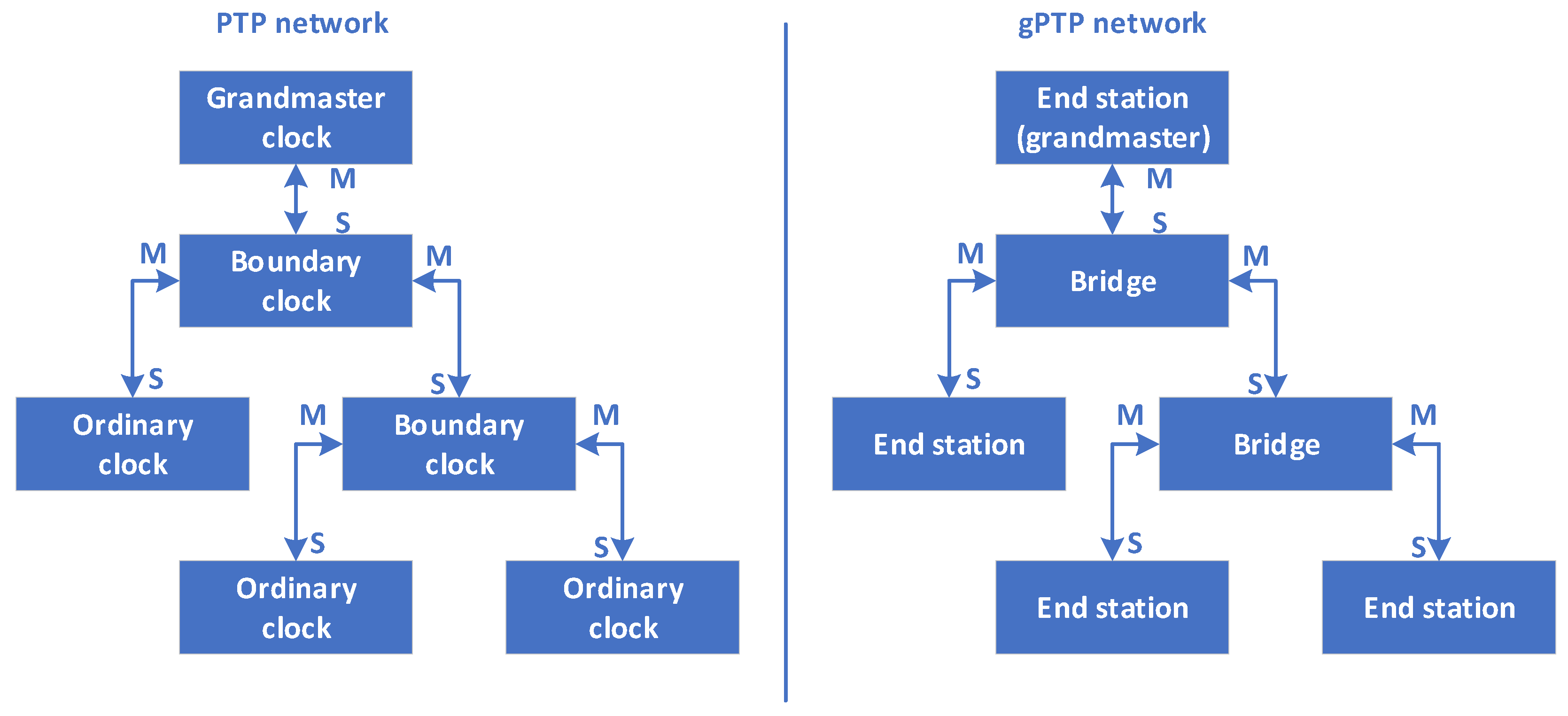
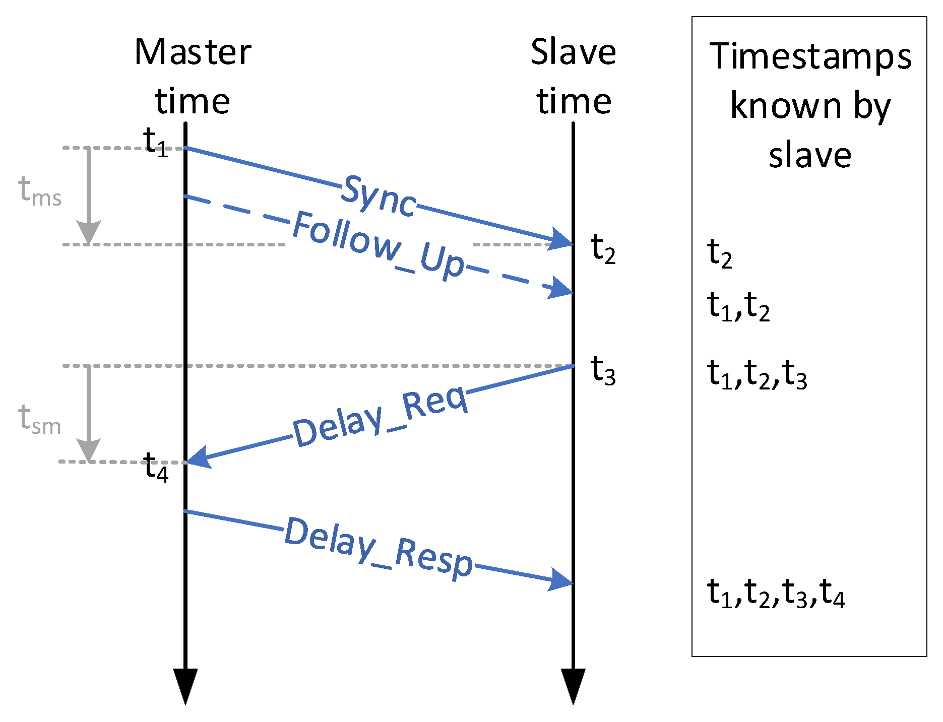
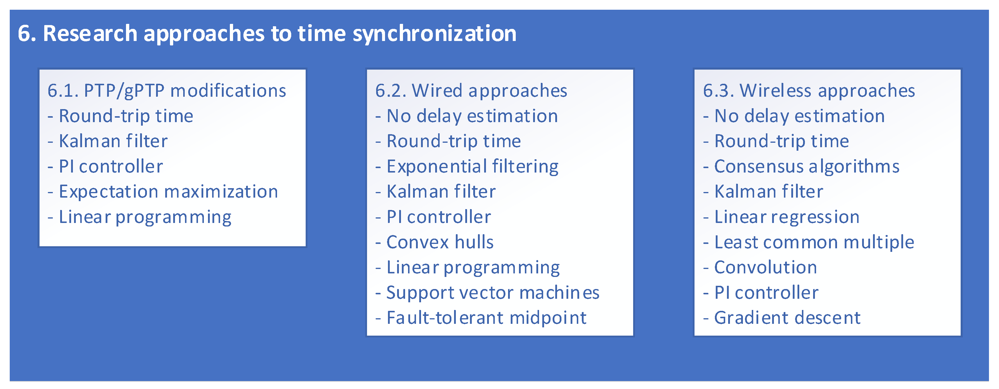
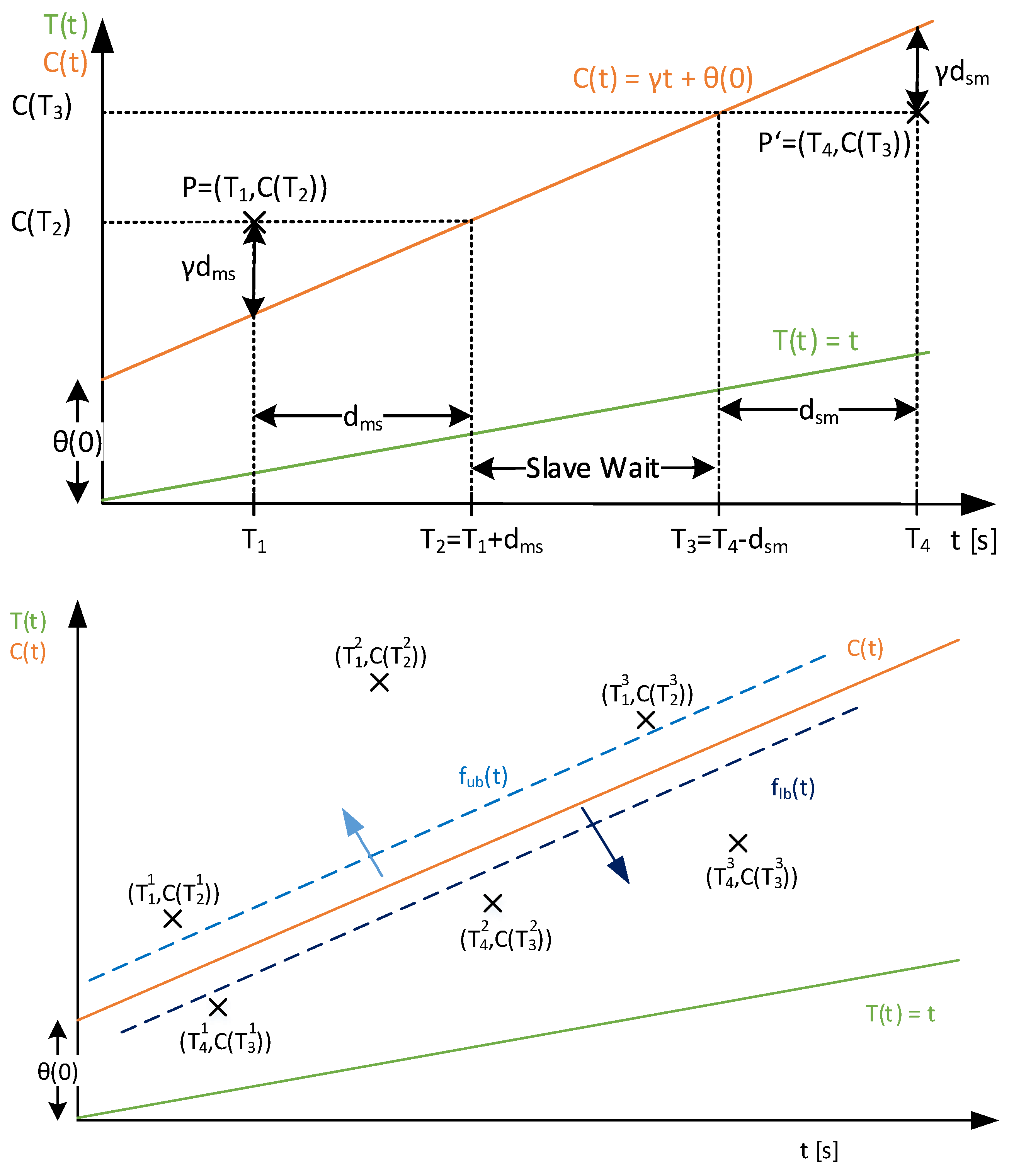
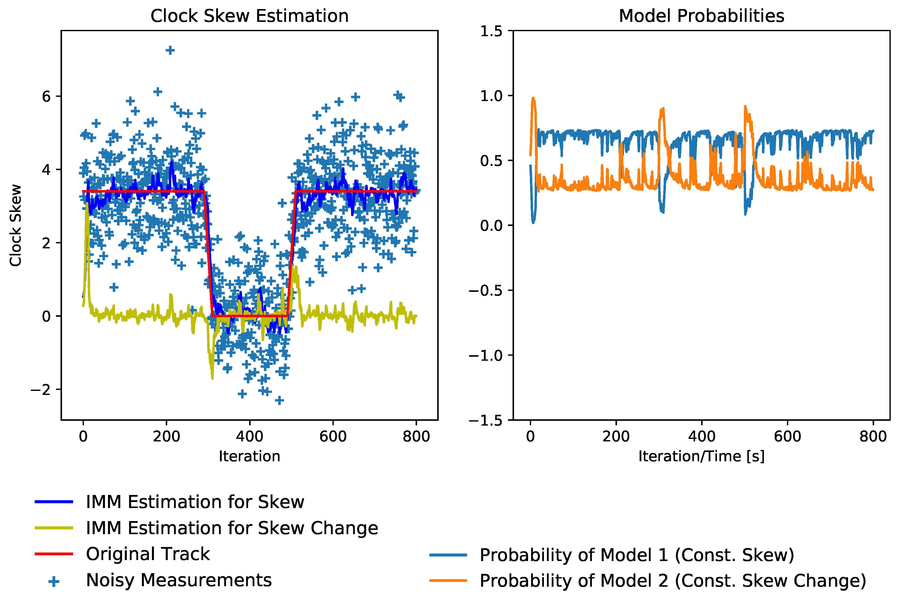
Table 1.
Overview of protocols for time synchronization. It shows their standard compatibility (SC), the estimation method used, the accuracy, as well as conditions and restrictions (MV = mean value, RTT = round-trip time, KF = Kalman filter, and PLL = phase-locked loop).
Table 1.
Overview of protocols for time synchronization. It shows their standard compatibility (SC), the estimation method used, the accuracy, as well as conditions and restrictions (MV = mean value, RTT = round-trip time, KF = Kalman filter, and PLL = phase-locked loop).
| Approach | SC | Estimator | Accuracy | Cond./restr. |
|---|---|---|---|---|
| NTP [47] | Yes | RTT | 1ms | None |
| PTP [48] | Yes | RTT | <1s | Custom HW |
| gPTP [49] | Yes | RTT | <1s | Custom HW |
| PTCP [50,51] | Yes | RTT | <1s | Custom HW |
| PTCP-KF [52] | Yes | KF | 20–200 ns | Eval. with Matlab |
| SyncE [53] | Yes | Offset: MV Freq.: PLL | Freq.: 4 ppm | Custom HW |
| c SyncE + Offset [54] | No | Offset: MV Freq.: PLL | NI Freq.: 4 ppm | Custom HW |
Table 2.
Overview of modifications to PTP or gPTP: The table shows their standard compatibility (SC), the estimation method used, the accuracy, as well as conditions and restrictions (KF = Kalman filter, NI = no information, PLL = phase-locked loop, SAGE = space altering generalized expectation-maximization, RTT = round-trip time, PI = proportional-integral (controller), and LP = linear programming).
| Approach | SC | Estimator | Accuracy | Cond./restr. |
|---|---|---|---|---|
| [67] | Yes (PTP) | RTT (ISR) | 10–100 ns | Testbed |
| [4] | Yes (PTP) | RTT | SW:20 s HW:10 ns–1 s | Analytically |
| [68] | No | RTT | <1 ns | Analytically + Sim. |
| White Rabbit [11,69,70] | Yes (PTP, IEEE 802.1Q, IEEE 802.3) | Offset:RTT Freq.: PLL | 200 ps | Testbed Custom HW |
| ReversePTP [71,72,73] | Yes | RTT | aprox. 8 ms (SW) | Testbed |
| [45] | Yes (PTP) | KF | NI | Sim. |
| [74] | Yes | KF | 100 ns–1 s | Analytically + Sim. |
| [75] | Yes (PTP) | KF | approximately 30 ns | Sim. |
| [76] | NI | KF + PI | 25 μs | Testbed |
| [77] | No | PI | 40–350 ns | Sim. + Testbed |
| [78] | NA | SAGE | NI | Sim. |
| PTP-LP [59] | Yes | LP/LR | approximately 100 ns | Sim. |
Table 3.
Overview of research approaches that primarily target wired scenarios. Their standard compatibility (SC), the estimation method used, the accuracy, as well as conditions and restrictions are shown (NI = no information, KF = Kalman filter, EF = exponential filtering, CH = convex hulls, ATD = averaged time differences, DSR = direct skew removal, SWI = sliding window, MV = mean value, HW-TS = hardware timestamps, GT = Gaussian traffic, ST = self-similar traffic, RTT = round-trip time, SLE = system of linear equations, LP = linear programming, IMM = interacting multiple model Kalman filter, RMSE = root mean square error , PI = proportional integral (controller), SVM = support vector machine, and FTM = fault-tolerant midpoint).
| Approach | SC | Estimator | Accuracy | Cond./Restr. |
|---|---|---|---|---|
| [35,36] | Yes (802.1Qcr) | None | None | Sim. |
| [82] | No | RTT | 11 ns | Testbed (Custom HW) |
| [83] | No | RTT | <7 s | Sim. (Custom HW) |
| DTP [57] | No | RTT | approximately 25 ns | (Custom HW) |
| TTE | ||||
| [84,85] | No | RTT | 10 ns–100 ns | Testbed (Custom HW) |
| PSPI-Sync [86] | No | RTT + SLE | approximately 100 s | Testbed |
| [87] | No | EF | 5–20 s | Analytically + Testbed |
| RADclock [88,89] | Almost (PTP) | EF | approximately 10 s | Testbed |
| [90] | No | KF | approximately 100 s | Testbed |
| [46] | Yes (NTP) | KF/LP/ATD | <30 ms (GT) <0.5 s (ST, LP) <0.75 s (ST, KF) <1.2 s (ST, ATD) | Sim. + Testbed |
| [91] | No | KF | <0.5 s | Sim. |
| [92] | No | KF | <1 s | Sim. |
| [93] | NI | KF | ca. 0.1 s | Sim. |
| [94] | No | KF | <100 s (RMSE) | Sim. |
| [95] | No | PI | 6.4 ns (RMSE) | Sim. |
| [96] | No | KF + PI | <18 ns | Testbed |
| [97] | No | CH | 1–1.6 ms | Sim. |
| [98] | NI | MW/DSR/SWI/CH | NI | Sim. |
| [99] | NI | LP | NI | Sim. |
| [100] | No | LP | NI | Analytically |
| SLMT [101] | No | LP + IMM | approximately 100 ns | Sim. |
| HYGENS [5] | Almost | |||
| (entirely SW) | SVM | approximately 100 ns | Testbed | |
| (HW-TS) | ||||
| [102] | Yes (FlexRay) | FTM | NI | Testbed |
Table 4.
Overview of research approaches that primarily target wireless scenarios: their standard compatibility (SC), the estimation method used, the accuracy, as well as conditions and restrictions are shown (NI = no information, CA = consensus algorithm, MSR = mean subsequence reduced, LCM = least common multiple, EKF = extended Kalman filter, CKF = custom Kalman filter, LR = linear regression, ISR = interrupt service routine, RTT = round-trip time, RMSE = root mean square error, KF = Kalman filter, PI = proportional integral (controller), GD = gradient descent, MA = moving average, DS = de facto standard, CFO = Carrier frequency offset, ECT = electronic counter theory).
| Approach | SC | Estimator | Accuracy | Cond./Restr. |
|---|---|---|---|---|
| FLIGHT [105] | No | None | approximately s | Testbed |
| [106] | No | Difference | <1 ms | Analytically + Sim. |
| RBIS [107] | Yes (802.11) | Difference | 0.2–3 s | Testbed |
| [108] | No | CFO + ECT | approximately 12–5 kHz (RMSE) | Sim. + Testbed |
| Pulsar [109] | NI | RTT | <5 ns | Testbed |
| TPSN [110] | NI | RTT | 16.9 s | Sim. + Testbed |
| GTSP [111] | Almost (entirely SW) | MW | 4–14 s | Sim. + Testbed (HW-TS + ISR) |
| [112] | NI | Sum | 76 s | Sim. + Testbed |
| R-Sync [113] | No | RTT | approximately 50 s | Sim. + Testbed |
| TCTS [104] | No | MW | 100–200 s | Sim. |
| [114] | No | CA+MSR | <100 ms | Sim. |
| [115] | NI | CA | NI | Analytically |
| [116] | Yes | CA | 100–1 ms | Analytically + Sim. |
| [117] | Yes | CA | approximately 1 s | Analytically + Sim. |
| CCS [118] | Yes | CA | NI | Sim. |
| TKDS [119] | NI | KF | NI | Sim. |
| [120] | NI | EKF | 0.5–34 ns | Sim. |
| [121] | NI | CKF | NI | Testbed |
| [66] | No | IMM-KF | <1 s (RMSE) | Sim. |
| EACS [14] | No | IMM-KF | 1 s–1 ms | Sim. + Testbed |
| DISTY [122] | Yes | KF | approximately 8 s | Analytically + Testbed |
| PulseSync [123,124] | NI | LR | approximately 2 s | Sim. + Testbed |
| FTSP [125] | Yes (DS) | LR | 1.48 s | Testbed |
| RBS [126] | Yes (DS, 802.11) | LR | 6.29 s | Sim. + Testbed |
| DualSync [127] | No | LR | <100 s | Sim. + Testbed |
| CESP [128] | Yes | LR/MA | approximately 2–3 s (MAC-TS) approximately 10 s (APP-TS) | Testbed |
| RTSP [7] | No | LR | approximately 0.2–0.3 s | Sim. |
| SPiRT [129] | NI | LCM | NI | Sim. + Testbed |
| WizSync [130] | NI | Convolution | approximately 0.12ms | Testbed |
| TACSC [131] | No | DSC | External: 15 s Internal: 160 s | Analytically + Sim. + Testbed |
| [132] | No | NI | 0.2 ms | Testbed |
| PISync [133] | Yes | PI | 20 s | Analytically + Testbed |
| GraDeS [134] | Yes | GD | <20 s | Analytically + Testbed |
Publisher’s Note: MDPI stays neutral with regard to jurisdictional claims in published maps and institutional affiliations. |
© 2020 by the authors. Licensee MDPI, Basel, Switzerland. This article is an open access article distributed under the terms and conditions of the Creative Commons Attribution (CC BY) license (http://creativecommons.org/licenses/by/4.0/).
Share and Cite
MDPI and ACS Style
Puttnies, H.; Danielis, P.; Sharif, A.R.; Timmermann, D. Estimators for Time Synchronization—Survey, Analysis, and Outlook. IoT 2020, 1, 398-435. https://0-doi-org.brum.beds.ac.uk/10.3390/iot1020023
AMA Style
Puttnies H, Danielis P, Sharif AR, Timmermann D. Estimators for Time Synchronization—Survey, Analysis, and Outlook. IoT. 2020; 1(2):398-435. https://0-doi-org.brum.beds.ac.uk/10.3390/iot1020023
Chicago/Turabian StylePuttnies, Henning, Peter Danielis, Ali Rehan Sharif, and Dirk Timmermann. 2020. "Estimators for Time Synchronization—Survey, Analysis, and Outlook" IoT 1, no. 2: 398-435. https://0-doi-org.brum.beds.ac.uk/10.3390/iot1020023