
ThriftyNets: Convolutional Neural Networks with Tiny Parameter Budget


1
ENS de Lyon, 69342 Lyon, France
2
Montreal Institute for Learning Algorithms (MILA), Montréal, QC H3C 3J7, Canada
3
IMT Atlantique, 29280 Plouzané, France
*
Author to whom correspondence should be addressed.
IoT 2021, 2(2), 222-235; https://0-doi-org.brum.beds.ac.uk/10.3390/iot2020012
Submission received: 29 January 2021
/
Revised: 23 March 2021
/
Accepted: 25 March 2021
/
Published: 30 March 2021
Abstract
:Deep Neural Networks are state-of-the-art in a large number of challenges in machine learning. However, to reach the best performance they require a huge pool of parameters. Indeed, typical deep convolutional architectures present an increasing number of feature maps as we go deeper in the network, whereas spatial resolution of inputs is decreased through downsampling operations. This means that most of the parameters lay in the final layers, while a large portion of the computations are performed by a small fraction of the total parameters in the first layers. In an effort to use every parameter of a network at its maximum, we propose a new convolutional neural network architecture, called ThriftyNet. In ThriftyNet, only one convolutional layer is defined and used recursively, leading to a maximal parameter factorization. In complement, normalization, non-linearities, downsamplings and shortcut ensure sufficient expressivity of the model. ThriftyNet achieves competitive performance on a tiny parameters budget, exceeding 91% accuracy on CIFAR-10 with less than 40 k parameters in total, 74.3% on CIFAR-100 with less than 600 k parameters, and 67.1% On ImageNet ILSVRC 2012 with no more than 4.15 M parameters. However, the proposed method typically requires more computations than existing counterparts.
1. Introduction
Convolutional Neural Networks (CNNs) have revolutionized the field of computer vision, providing consistent state-of-the-art results in a wide range of tasks, from image recognition to semantic segmentation. This increase in performance was accompanied by an increase in the depth, size and overall complexity of the corresponding models. It is not unusual to encounter models with hundreds of layers and tens of millions of parameters. This is even more true in the field of Natural Language Processing where very large models usually lead to the best performance.
There are multiple reasons why it would be desirable to reduce the size of CNNs. For example, for some applications, it is required to deploy systems on resource-constrained hardware (e.g., IoT) or to provide real-time predictions (e.g., assisted surgery, autonomous vehicles…). More generally, deep learning systems are often deployed as black boxes trained on huge available datasets, and are therefore lacking understandability and interpretability: reducing the number of parameters can help in visualizing and explaining decisions. Additionally, datacenters are increasingly used for deep learning, and their impact on the environment is becoming a concern.
For all these reasons, there have been a significant amount of works aiming at reducing the size and computational cost of CNNs. To cite a few, some works propose to prune the connections in deep learning systems so as to reduce their numbers [1]. Other works propose to distillate the knowledge from large architecture to smaller ones [2]. It is also possible to focus on reducing the bit precision of weights and/or activations [3] or to factorize some of the operations [4,5]. Finally, a lot of efforts have been dedicated to finding efficient architectures [6,7,8].
A key difficulty in the field is tied to the fact that there are multiple metrics to act upon, and a lot of possible hardware targets, on which some methods might not be applicable. Throughput, latency, energy, power, flexibility and scalability are among the most discussed ones in the literature. In this work, we focus on reducing the number of parameters of architectures, which is usually strongly connected to the memory usage of the model. In this area, factorizing methods, which identify similar sets of parameters and merge them [4], are particularly effective, in that they considerably reduce the number of parameters while maintaining the same global structure and number of flops. Our contribution can be thought of as a factorization technique.
In this work, we propose to introduce a new factorized deep learning model, in which the factorization is not learned during training, but rather imposed at the creation of the model. We call these models ThriftyNets, as they typically contain a very constrained number of parameters, while achieving top-tier results on standard classification vision datasets. The core idea we introduce consists of recycling the same convolution to be applied a large number of times when processing an input element. In more details, we introduce ThriftyNets, a new family of deep learning models that are designed with a fixed number of parameters and variable depths and flops. To report ThriftyNet perormance, we perform experiments on standard vision datasets and show that we are able to outperform current deep learning solutions for tiny parameters budget. We also design experiments to stress the impact of the hyperparameters of the proposed models on the accuracy and the flops of obtained solutions.
The outline of the paper is as follows. In Section 2 we present related work and discuss the context of our proposed method. In Section 3 we introduce the proposed methodology and discuss the role of hyperparameters on the total number of parameters. In Section 4 we perform experiments using standard vision datasets and compare the proposed method with existing alternative architectures. Section 5 is a conclusion.
2. Related Work
Many different approaches were explored in the field of neural network compression, always with the goal of finding the best trade-off between resource efficiency and model accuracy. Most of those methods are orthogonal to one another, meaning that they can be used all together on the same model. For example, pruning, quantization and distillation methods could be applied to ThriftyNets for even smaller model sizes. In the next paragraphs, we introduce the main contributions to the field, grouped by the type of compression they perform.
2.1. Pruning
Pruning, first introduced by [9], aims at deleting parameters, channels, or parts of a network while preserving the global performance [10]. While setting single parameters to zero induces sparsity in both the intermediate representations and parameter tensors, deleting complete channels is harder to achieve with good performance, yet allows faster inference time and less resource consumption. Pruning can be performed once and for all after training, in order to reduce the model’s size [1,9,11,12], or during training [5,13] to impact training time as well. In the first case, the stress is put on defining a metric for deleting the least useful neurons or channels. In the latter, mechanisms are designed in order to force the network to abandon the use of some of its parameters during training. Pruning can be applied to the proposed ThriftyNets to reduce their number of parameters.
2.2. Quantization
While standard floating-point values have 32 bits of precision, many works have experimentally demonstrated that neural networks do not lose a lot of performance when their parameters are restricted to a small set of possible values [14], up to binary neural networks with only two possible values and one bit storage for each parameter [15]. Reducing precision allows models to be more compact by a great factor, and allows implementation on dedicated low precision hardware [16,17]. Like pruning, quantization can be performed after training through a transformation of the parameters [18,19,20], or during training [3]. Despite the fact quantization can greatly benefit the memory usage of CNNs, it usually does not reduce the number of parameters and is therefore quite different from the aim of this paper.
2.3. Distillation
Distillation techniques consist of training a deep neural network, termed ‘student’, to reproduce the outputs of another model, termed ‘teacher’, with the student being typically smaller than the teacher. While initially only considering the final output of the teacher model [2], methods evolved to take into account intermediate representations [21,22]. Distilling a model into itself, or self-distillation has also proven to be effective when iterated [23]. While individual knowledge distillation focused on the student mimicking the outputs of the teacher, relational knowledge distillation [24,25] made it reproduce the same relations and distances between training examples, yielding a better representation of the latent space for the student, and better generalization capabilities.
2.4. Efficient Scaling
While the diversity of datasets in computer vision does not cease to increase, some works are focused on the re-usability of architectures that perform well on specific tasks. Mainly, the resolution and complexity of the input image play a great role in the minimal number of parameters required to achieve good performance. While it is possible to scale architectures by adding layers (depth increase) [26] or by adding filters (width increase) [6,27], a correct balance between those hyperparameters has been shown to lead to better results [8].
2.5. Factorization
Factorization consists of reusing parameters, channels or whole parts of the network several times, thus effectively reducing its size compared to a counterpart where the repeated parts would be made of distinct elements. Parameters can be grouped by values, and accessed through an indirection table [4], in approaches that are often coupled with quantization [28]. Convolution kernels of great size can be factorized into smaller kernels before training [7,29] or using matrix factorization after training [19]. The proposed architectures can be thought of as heavily factorized CNNs.
2.6. Recurrent Residual Networks as ODE
Since the initial proposal of residual networks [26], many works have studied them theoretically, observing that the forward pass of a residual network resembles the explicit Euler scheme of an ordinary differential equation [30,31,32]. The question of stability, invertibility and reusability of the convolutional filters became central [33,34]. Experiments were conducted on recurrent residual networks with a single filter iterated over time [35]. Those studies provide theoretical insight on why reusing filters at different depths can be effective. The proposed method is highly inspired by those works.
3. Methodology
3.1. Context
CNNs form a family of Deep Neural Networks which parameters are mainly arranged in convolutional layers. Such layers are determined by two tensors and , corresponding to the kernels and biases parameters respectively. Denoting by the number of input channels, the number of output channels, a the kernel width and b the kernel height, the cardinality of can be written as , while has cardinality .
In most cases, architectures become wider in their deep layers, where the spatial dimension of processed signals is reduced. As a consequence, most of the parameters are contained in the deep layers, while the number of operations is almost evenly distributed along the architecture [26]. In an effort to reduce the number of parameters in deep convolutional neural networks, it is therefore usual to target the deep layers in priority. This is in contradiction with the fact that the number of parameters scales quadratically with the depth of the architecture in many models. This is even more problematic since state-of-the-art results often rely on the use of (very) deep neural networks.
In order to remove this dependency, we propose to share kernels between layers, from the input to the output of the considered architecture. Similar ideas were proposed in previous works [35]. As a result, the proposed architectures can be scaled to any depth with little impact on the total number of trainable parameters.
3.2. Thrifty Networks
Consider a problem in which the aim is to associate an input tensor with an output through the network function f. This network function is trained using a variant of the stochastic gradient descent algorithm to minimize a loss function over a dataset .
We propose to define a convolutional layer , parametrized by weights , and to build a deep neural network using only this layer iteratively applied T times on successive latent representations of the input. Note that we do not use convolution with bias in this work.
This architecture, called ThriftyNet, is then defined by the following recursive sequence:
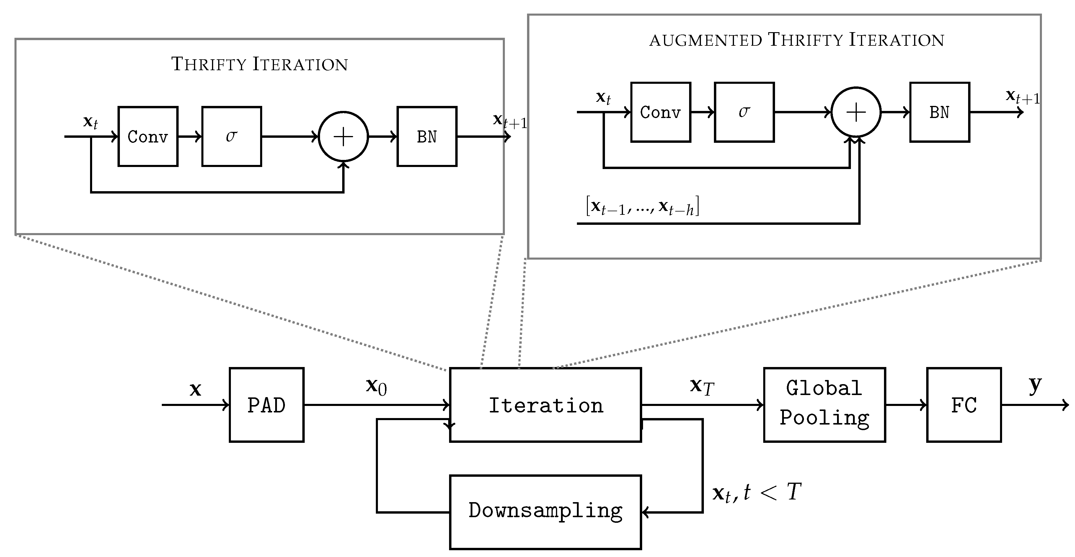
, where PAD creates extra channels filled with constant values to extend the dimension of , BN is a batchnorm layer, is a downsampling operation (typically achieved with strides or pooling) or the identity function, and FC is a final fully connected layer. Note that the PAD function is only used on the input of the network as a mean to adapt the input tensor shape to the convolutional layer. Note that an overview of the proposed method is depicted in Figure 1.
Several classical activation functions were considered in this algorithm. In our case, not only do they break the linearity, they also play an important role in regularizing the norm of the activation tensor. We found that the hyperbolic tangent and ReLU yielded the best results in term of accuracy. However, for the purpose of implementing this algorithm onto specific hardware, we focused on rectified linear units (ReLU).
Note that convolutions can be applied to inputs of any spatial dimensions, which is why we can reduce the spatial dimension of the inputs throughout the process.
3.3. Augmented Thrifty Networks
In order to boost the performance of thrifty networks, we add a shortcut mechanism, where activations from previous iterations can be added from the past. This augmented thrifty network adds parameters on top of a regular thrifty network, with h being a hyperparameter representing how many steps in history are kept in memory when processing a new iteration. They are grouped in a matrix . Those parameters are the coefficients weighting the contribution from past activations at each step. In augmented thrifty nets, Equation (1) is replaced as follows:
, where ◯ denotes the composition operator. Previous activations are added only if .
Adding contributions from the past lead to better performance of the architecture on every task at the expanse of only a handful of additional parameters. However, the cost of computation is slightly increased, as well as the memory requirements to store previous activations. This trade-off will be discussed in the experiments section.
3.4. Pooling Strategy
Pooling has two notables effects: firstly, it diminishes the number of computations made by one iteration which significantly increases the speed of a forward pass in the model. Secondly, it allows the convolutional filter to take effect into larger regions of the initial images. In the augmented thrifty network, pooling is applied to every elements in the history, in order to guarantee size compatibility. The pooling positions are set as hyperparameters, and various strategies are possible and discussed in the experiments.
A key property of convolutional layers is that they are defined independently of the input dimensions. As such, we can reuse the same convolutional on inputs of various dimensions, starting from the full spatial resolution to strongly downscaled representations.
As a consequence, once the hyperparameters of the convolution are fixed, a ThriftyNet is characterized by an integer sequence , where denotes the downsampling that occurs at step t (1 means by convention that no downsampling is performed at this step).
3.5. Grouped Convolutions
In our models, we found that using grouped convolutions can lead to better performance for some tasks. Recall that a group convolution is obtained by splitting the input tensor along the feature maps axis, and performing computations on each resulting slice concurrently with independent kernels. In more details, in some experiments we design convolutions that are obtained by composing two elementary convolutions: the first one uses a kernel-size and as many groups as feature maps in the input. The second one uses kernel-size of 1 and only one group. As a result, the first convolution exploits the spatial structure of the input, but treats each feature maps independently, whereas the second convolution disregards the spatial structure but mixes feature maps. The total number of parameters in the weights of such a convolution is therefore .
3.6. Hyperparameters and Size of the Model
In Table 1 we recap the hyperparameters to define ThriftyNet and their augmented version. These hyperparameters are recalled or defined in the following list:
- The number of filters f in the convolutional layer
- The dimension of the convolution kernel
- The number of iterations T
- The number of steps h to consider when performing shortcuts from previous activations
- The downsampling sequence
3.7. Depth and Abstraction
One could believe that ThriftyNets are not likely to reach top performance, as generic deep neural networks are believed to produce more abstract features as we go deeper in their architectures, whereas ThriftyNets use the same features at any depth. We argue that specialized features would likely occur if objects to recognize would have very similar scales. For challenging vision datasets, it is likely that the scale changes from an image to the next. In this case, it is desirable to retrieve similar features at various depths in the architecture, because increasing depth leads to encompassing increasingly larger local receptive fields. As such, ThriftyNets are likely to yield increased invariance to scale, which probably explains in part its ability to reach good performance despite its few parameters.
4. Experiments
In this section, we explore the performances obtained with various values of hyperparameters, namely the total number of iterations T, the number of downsamplings performed, the history, and the number of filters f, which is directly linked to the number of parameters.
Experiments were performed on CIFAR-10, CIFAR-100, SVHN and ImageNet ILSVRC 2012. CIFAR-10 and CIFAR-100 [36] are datasets of tiny colored images of 32 × 32 pixels. They contain both 50,000 samples for training and 10,000 samples for test. CIFAR-10 is made of 10 classes, whereas CIFAR-100 contains 100 classes. Note that state-of-the-art accuracy is 98.9% on CIFAR-10 and 91.70% on CIFAR-100 using EfficientNet-B7 [8] (64 M parameters). SVHN is a dataset of digit classification from pictures of house numbers. Images are also of size 32 × 32 and present up to three digits in them. The classification task consists in identifying the central digit. The state-of-the-art performance without data augmentation was achieved by a Wide-ResNet-16-8 [27] with 98.46% accuracy. ImageNet ILSVRC 2012 is a dataset containing high resolution images, and made of 1000 classes, where each class contains about 1000 training images and 50 images for test. The state of the art Top 1 accuracy is 88.61% achieved by EfficientNet-L2-475 [37].
We use Stochastic Gradient Descent as an optimizer, and a starting learning rate of and dividing it by 10, usually at epochs 50, 100 and 150, for a total of 200 epochs when considering CIFAR-10, CIFAR100 and SVHN, and a starting learning rate of and dividing it by 10, usually at epochs 30 and 60, for a total of 90 epochs when considering ImageNet ILSVRC 2012.
4.1. Impact of Data Augmentation
In this experiment, we aim at stressing the effect of data augmentation on the accuracy of proposed networks. Note that when we work with tiny networks, regularization techniques like heavy data augmentation, mixup or cutmix, designed to help very expressive networks to achieve better generalization performance, have little to no effect, as observed in our experiments. In Table 2, we report the performance on test sets we obtained when using an augmented ThriftyNet with 40 k parameters and 20 iterations trained on CIFAR-10 as described in Section 4. We observe very little impact in using more advanced techniques of data augmentation. We hypothesize that thrifty architectures are less likely to cause overfitting because of the very constrained number of parameters. On SVHN, a 20 k parameter ThriftyNet, trained with Auto Augment [38] and Cutout of size 8 [39] achieves 97.25% accuracy, compared to the 96.59% of the same architecture trained on the raw dataset.
As a result, and to fairly compare the proposed method with other state-of-the-art solutions, we use in the following experiments standard augmentation consisting of horizontal flips (for CIFAR only) and random crops. Note that when considering ImageNet ILSVRC 2012, we use standard data augmentation defined in [42].Note that int the following experiments, the same data augmentation is used for all methods.
4.2. Comparison with Standard Architectures
We then compare in Table 3 and Table 4 the performance of the proposed ThriftyNet architectures to standard ones found in the literature, resp. on CIFAR-10 and CIFAR-100. Note that Macs refers to the number of multiplications required to process one input and classify it.
The first observation that we can draw from Table 3 and Table 4 is that ThriftyNets present competitive results with the literature for a tiny parameter budget. The augmented ThriftyNet we use on CIFAR-10 achieves up to 91% accuracy while using less than 40 K parameters in total. The only size-comparable architecture we found is the one introduced in [35], but its accuracy is significantly lower than that of the ThriftyNets. Since it is not completely fair to compare architectures that target different accuracies, we run an additional experiment in which we scale down DenseNet-BC and Resnet so that they contain a comparable number of parameters. More precisely, we proportionally reduce the number of feature maps of every single convolutional layer in the considered architectures until reaching the targeted number of parameters. We obtain that DenseNet-BC achieves 87.91% accuracy, and Resnet 86.72% accuracy. Again, we observe a significant drop in accuracy compared to ThriftyNets. We conclude that for the same parameter budget, The proposed architecture achieves better accuracy than other counterparts.
To perform comparisons on ImageNet ILSVRC 2012, we had to adapt the proposed ThriftyNets. Indeed, since inputs are typical of high resolutions, the first filters require too many computations. We thus used a combination of a Resnet18 for processing the first layers of the architecture with a ThriftyNet for the last ones, when the spatial resolution has significantly reduced. We compared with a scaled-down Resnet18 (small-Resnet18). Table 5 shows that when replacing the last B building blocks by ThriftyNet, we achieve comparable accuracy to the Resnet baselines while considerably reducing the number of parameters. Note that this gain in the number of parameters comes with the disadvantage of a significant increase in the number of multiplications.
What we draw from these experiments is that when the parameter budget is very constrained, ThriftyNets appear as an interesting choice. For CIFAR-100, the proposed augmented ThriftyNet architecture achieves 74.37% accuracy, which is competitive regarding its 600 k parameters in total, and for ImageNet, it achieves 67.1% accuracy while requiring only 4.15 M parameters.
However, let us point out that this performance comes at the expense of the number of operations performed by the network. Since ThriftyNets apply the same convolutional filter at each iteration, first iterations using both the full depth of the filter and the full resolution of images are very costly. We investigate this limitation later in this section. In brief, we can say that ThriftyNets represents an efficient solution when considering the number of parameters to be constrained, but it is outperformed by other state-of-the-art architectures when considering complexity (i.e., number of operations).
4.3. Factorization and Filter Usage
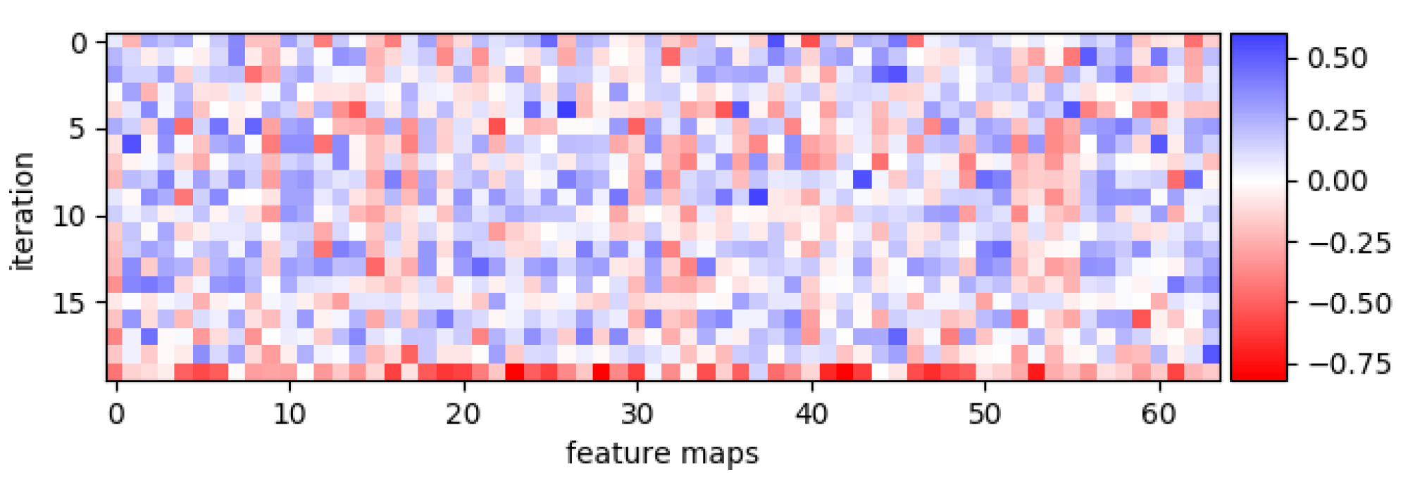
Iterating over the same convolutional filter on a ThriftyNet that presents downsamplings means that the architecture is offered the possibility to reuse filters over different spatial resolutions of the inputs. One could then imagine that the optimization scheme would associate some filters with wide spatial representations and some with deeper iterations in the network. In Figure 2, we plot the mean activation of the filters over the training set of CIFAR-10 for each iteration, for a trained augmented ThriftyNet with 64 filters and 20 iterations. We observe that no clear pattern appears in the activation of the filters, from which we deduce that they are being consistently used at every iteration.
4.4. Efficient ThriftyNets
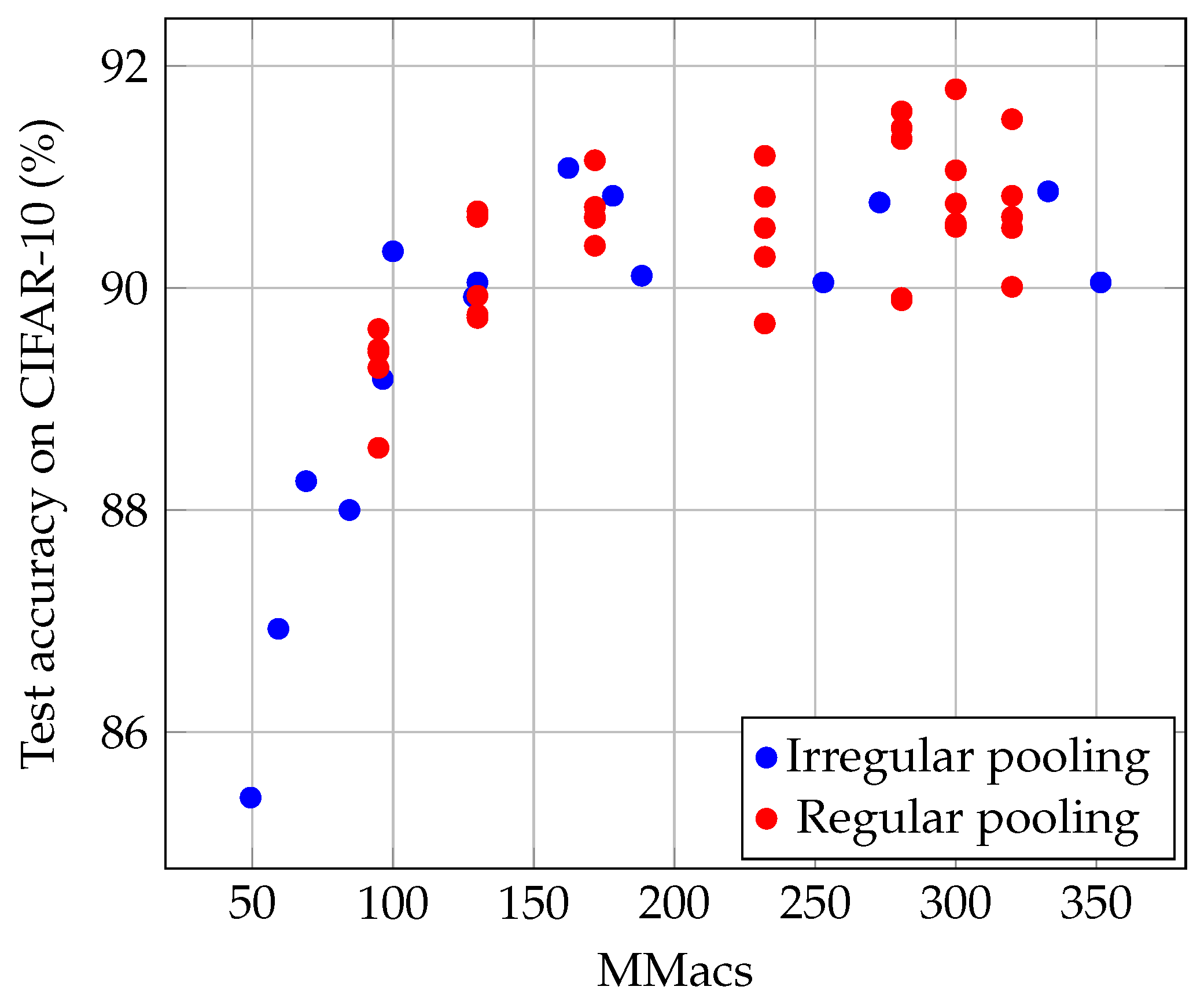
In an effort to reduce the impact of the computational cost of the first iterations, it can be beneficial to perform downsamplings sooner than later. In the last experiments, we used a regular spacing of downsamplings. However, here we consider performing them at any iteration. On CIFAR-10, we were able to obtain an accuracy of 85.35% for a total of 49 M Macs, while the regular pooling version achieves a mean of 90.15% for 130 M Macs.
This sheds light on a trade-off in neural network architectures, where a small number of parameters can be compensated by a large number of computations. In Figure 3, we illustrate this phenomenon by plotting the final test accuracy on CIFAR-10 for various ThriftyNets as a function of their Mac count, for a fixed number of parameters (40 k). We distinguish two possibilities: in blue, we depict what happens when performing irregularly spaced downsamplings and in orange what happens when the total number of iterations varies but downsamplings are regularly spaced.
Interestingly, the two solutions we compare to reduce the number of operations seem to lead to similar behaviors in terms of the trade-off between Macs and accuracy. While irregular downsamplings may lead to more iterations for the same Macs budget, we hypothesize that reducing the number of iterations on high-resolution intermediate representations can lead to significant drops in accuracy.
4.5. Effect of the Number of Iterations
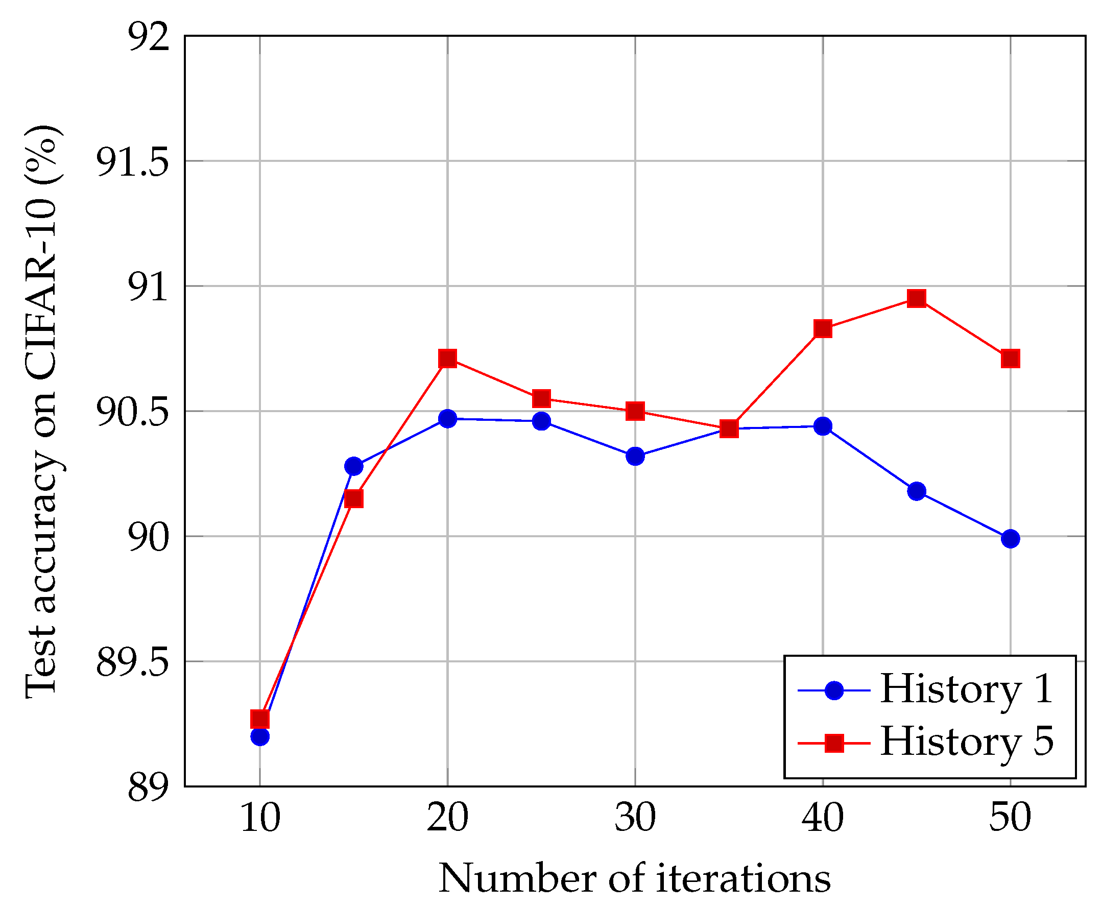
Another important hyperparameter to design ThriftyNets is the number of iterations we use. Normally, this hyperparameter directly influences the number of parameters in the architecture (c.f. Table 1). As a consequence, it is difficult to analyze the influence of T. In Figure 4, we report the test-set accuracy of ThriftyNets and augmented ThriftyNets when varying the number of iterations T, but for a fixed parameters budget of 40 k that we reach by tuning the number of feature maps f accordingly.
First, let us point out that extreme values of T would necessarily lead to poor performance. Indeed, choosing would lead to a shallow network with poor generalization abilities. Choosing a too-large T would cause the number of filters to become too small to expect good performance. What we observe in the experiments is that the choice of T could be more tightly restricted since in the case of ThriftyNets, and lead to poorer performance than values in between. Yet, in the range , we observe that tuning the number of iterations for a given parameters budget has little influence on overall performance.
4.6. Effect of the Number of Filters
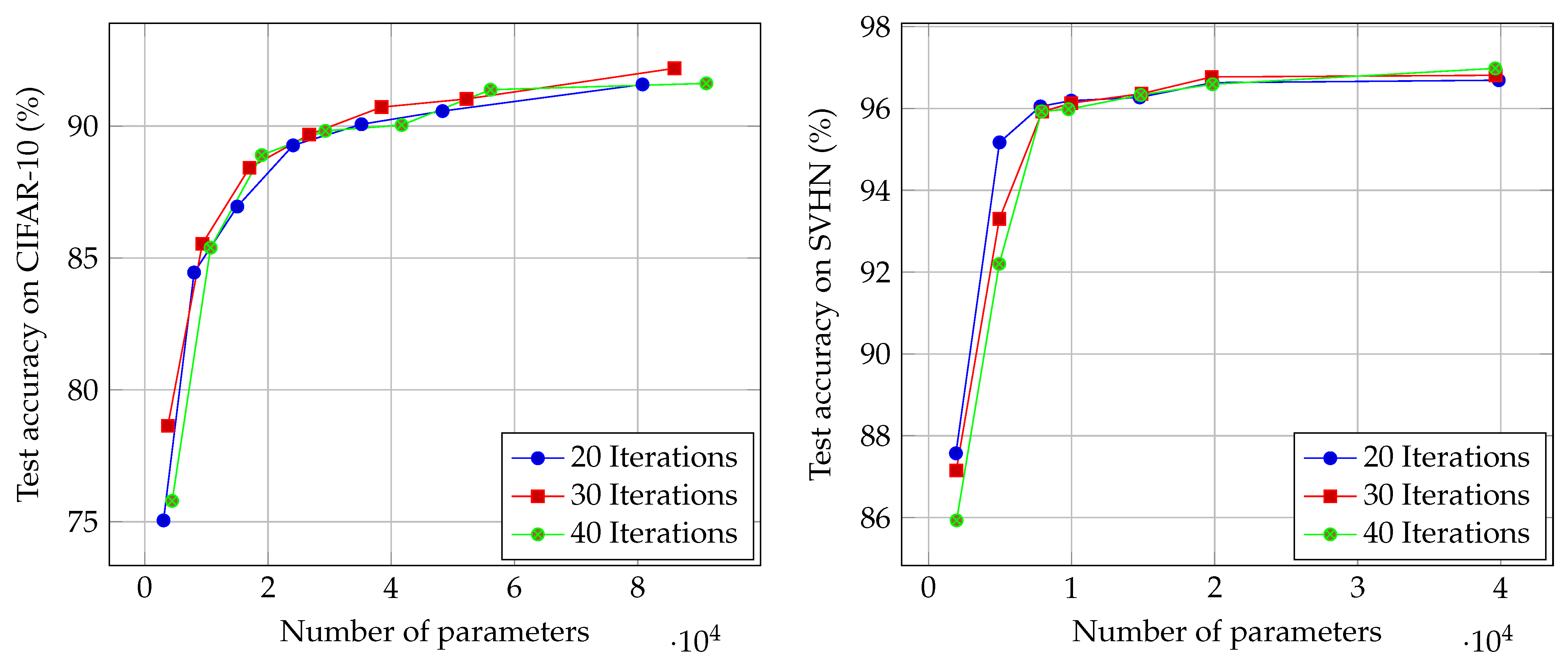
Next, we investigate the evolution in accuracy when the number of filters f increases. Of course, increasing the number of filters leads to more parameters, as shown in Table 1. Figure 5 shows the evolution of accuracy for CIFAR-10 and SVHN as a function of the number of parameters, obtained when varying f. In both cases, we observe that the trade-off between the number of parameters and accuracy is not linear: reaching 1% extra accuracy can be very costly in terms of the required number of parameters, if the accuracy is already high. This trade-off is even sharper in the case of SVHN where we observe a two-step phenomenon, where accuracy is first increased quickly but then saturates. We think that this is a consequence of the difficulty of considered datasets: achieving 93% accuracy on CIFAR-10 is significantly harder than in the case of SVHN.
4.7. Effect of the Number of Downsamplings
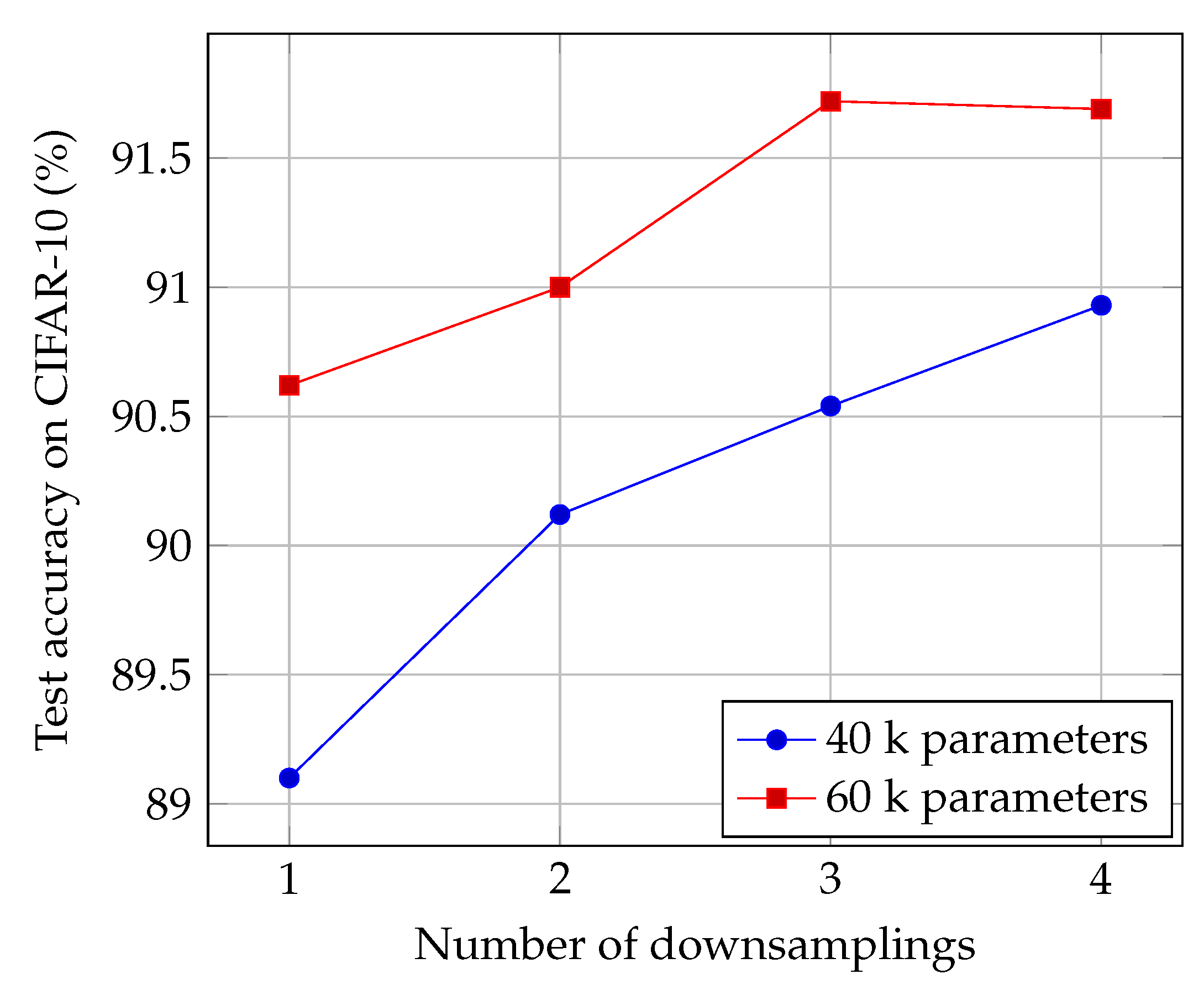
Then, we perform an ablation experiment for investigating the importance of pooling in our architecture. We fix the number of parameters and number of iterations, and we report in Figure 6 the evolution of the accuracy as a function of the number of downsamplings. Without surprise, we observe that the more downsamplings, the better the accuracy.
Interestingly, increasing the number of downsamplings has a decreasing consequence on the number of operations that are performed. So contrary to what we reported in Figure 3, here increasing the number of downsamplings is beneficial to both computational complexity and accuracy.
4.8. Freezing the Shortcut Parameters in an Augmented ThriftyNet
In most modern architectures, shortcut mechanisms consist in adding previous activations to the current one, thus bypassing some of the layers. While they are often fixed and involve only one past activation, we designed augmented ThriftyNets to take into account the h last activations, weighted by parameters . This is designed with the hope that the optimization of leads ThriftyNet into finding the most efficient architectures, and avoid the introduction of additional hyperparameters and user priors.
To demonstrate this phenomenon, we perform an ablation experiment. We train an augmented ThriftyNet with an additional loss , designed to make the shortcut parameters converge to 0 or 1. More precisely:
We perform 150 epochs of training, with being multiplied by after every forward and backward pass of a batch (500 batches per epoch, , ). Parameters are then binarized using a threshold at 0.5. From this, we train for 150 additional epochs:
- (a)
- The same model without resetting the other parameters
- (b)
- The same model starting from the same initialization
- (c)
- The same model starting from another (random) initialization
Table 6 sums up the results obtained on CIFAR-10 for this experiment. We observe that the baseline gives the best results. This was expected since shortcuts remain free parameters that can take values other than 0 or 1. Once shortcuts have been fixed and binarized, training from the same initialization is what ranks next. In our experiments, it evens outperforms fine-tuning, as the binarization step has a dramatic effect on the accuracy. Training from scratch with random initialization and the same shortcuts leads to a drop of about 1% accuracy.
5. Conclusions
We introduced ThriftyNet, a convolutional neural network architecture that explores the limits of layer factorization and the efficacy of architectures with tiny parameter count. Based around a single convolutional layer, ThriftyNets iterate over this layer, alternating convolution operations with non-linear activation, batch normalization, downsampling through pooling operations and weighted sums with results from previous iterations. This leads to a very compact architecture that achieves competitive results regarding the trade-off between the total number of parameters and accuracy. Such a solution would be beneficial to memory-constrained systems. Moreover, since the introduced architecture uses sequentially the same layer, it may ease the hardware implementation of DNNs when considering limited resources embedded systems that have to use the same hardware sequentially to compute different operations. In future work, we consider investigating other strategies to mitigate the large computational cost of ThriftyNets.
Author Contributions
Conceptualization and methodology: G.C., G.B.H. and V.G.; Software: G.C.; Supervision: V.G. Writing: G.C. and V.G.; Review and Editing: G.B.H. All authors have read and agreed to the published version of the manuscript.
Funding
This research received no external funding.
Institutional Review Board Statement
Not applicable.
Informed Consent Statement
Not applicable.
Data Availability Statement
The Cifar10 and Cifar100 datasets are provided by the university of Toronto https://www.cs.toronto.edu/~kriz/cifar.html (accessed on 30 March 2021). The ImageNet dataset is available online http://image-net.org/ (accessed on 30 March 2021). No other data was used in this work.
Conflicts of Interest
The authors declare no conflict of interest.
References
- Han, S.; Pool, J.; Tran, J.; Dally, W. Learning both weights and connections for efficient neural network. In Proceedings of the Advances in Neural Information Processing Systems, Montreal, QC, Canada, 7–10 December 2015; pp. 1135–1143. [Google Scholar]
- Hinton, G.; Vinyals, O.; Dean, J. Distilling the knowledge in a neural network. arXiv 2015, arXiv:1503.02531. [Google Scholar]
- Courbariaux, M.; Bengio, Y.; David, J.P. Binaryconnect: Training deep neural networks with binary weights during propagations. In Proceedings of the Advances in Neural Information Processing Systems, Montreal, QC, Canada, 7–10 December 2015; pp. 3123–3131. [Google Scholar]
- Wu, J.; Wang, Y.; Wu, Z.; Wang, Z.; Veeraraghavan, A.; Lin, Y. Deep k-Means: Re-Training and Parameter Sharing with Harder Cluster Assignments for Compressing Deep Convolutions. arXiv 2018, arXiv:1806.09228. [Google Scholar]
- Han, S.; Mao, H.; Dally, W.J. Deep compression: Compressing deep neural networks with pruning, trained quantization and huffman coding. arXiv 2015, arXiv:1510.00149. [Google Scholar]
- Howard, A.G.; Zhu, M.; Chen, B.; Kalenichenko, D.; Wang, W.; Weyand, T.; Andreetto, M.; Adam, H. Mobilenets: Efficient convolutional neural networks for mobile vision applications. arXiv 2017, arXiv:1704.04861. [Google Scholar]
- Iandola, F.N.; Han, S.; Moskewicz, M.W.; Ashraf, K.; Dally, W.J.; Keutzer, K. SqueezeNet: AlexNet-level accuracy with 50x fewer parameters and <0.5 MB model size. arXiv 2016, arXiv:1602.07360. [Google Scholar]
- Tan, M.; Le, Q.V. Efficientnet: Rethinking model scaling for convolutional neural networks. arXiv 2019, arXiv:1905.11946. [Google Scholar]
- LeCun, Y.; Denker, J.S.; Solla, S.A. Optimal brain damage. In Proceedings of the Advances in Neural Information Processing Systems, Denver, CO, USA, 26–29 November 1990; pp. 598–605. [Google Scholar]
- Blalock, D.; Ortiz, J.J.G.; Frankle, J.; Guttag, J. What is the State of Neural Network Pruning? arXiv 2020, arXiv:2003.03033. [Google Scholar]
- Li, H.; Kadav, A.; Durdanovic, I.; Samet, H.; Graf, H.P. Pruning filters for efficient convnets. arXiv 2016, arXiv:1608.08710. [Google Scholar]
- Luo, J.H.; Wu, J.; Lin, W. Thinet: A filter level pruning method for deep neural network compression. In Proceedings of the IEEE International Conference on Computer Vision, Venice, Italy, 22–29 October 2017; pp. 5058–5066. [Google Scholar]
- Hacene, G.B.; Lassance, C.; Gripon, V.; Courbariaux, M.; Bengio, Y. Attention based pruning for shift networks. arXiv 2019, arXiv:1905.12300. [Google Scholar]
- Gupta, S.; Agrawal, A.; Gopalakrishnan, K.; Narayanan, P. Deep learning with limited numerical precision. In Proceedings of the International Conference on Machine Learning, Lille, France, 6–11 July 2015; pp. 1737–1746. [Google Scholar]
- Hubara, I.; Courbariaux, M.; Soudry, D.; El-Yaniv, R.; Bengio, Y. Binarized neural networks. In Proceedings of the Advances in Neural Information Processing Systems, Barcelona, Spain, 5–10 December 2016; pp. 4107–4115. [Google Scholar]
- Merolla, P.A.; Arthur, J.V.; Alvarez-Icaza, R.; Cassidy, A.S.; Sawada, J.; Akopyan, F.; Jackson, B.L.; Imam, N.; Guo, C.; Nakamura, Y.; et al. A million spiking-neuron integrated circuit with a scalable communication network and interface. Science 2014, 345, 668–673. [Google Scholar] [CrossRef]
- Farabet, C.; Martini, B.; Corda, B.; Akselrod, P.; Culurciello, E.; LeCun, Y. Neuflow: A runtime reconfigurable dataflow processor for vision. In Proceedings of the CVPR 2011 Workshops, Colorado Springs, CO, USA, 20–25 June 2011; pp. 109–116. [Google Scholar]
- Gong, Y.; Liu, L.; Yang, M.; Bourdev, L. Compressing deep convolutional networks using vector quantization. arXiv 2014, arXiv:1412.6115. [Google Scholar]
- Denton, E.L.; Zaremba, W.; Bruna, J.; LeCun, Y.; Fergus, R. Exploiting linear structure within convolutional networks for efficient evaluation. In Proceedings of the Advances in Neural Information Processing Systems, Montreal, QC, Canada, 8–13 December 2014; pp. 1269–1277. [Google Scholar]
- Choi, Y.; El-Khamy, M.; Lee, J. Towards the limit of network quantization. arXiv 2016, arXiv:1612.01543. [Google Scholar]
- Romero, A.; Ballas, N.; Kahou, S.E.; Chassang, A.; Gatta, C.; Bengio, Y. Fitnets: Hints for thin deep nets. arXiv 2014, arXiv:1412.6550. [Google Scholar]
- Koratana, A.; Kang, D.; Bailis, P.; Zaharia, M. Lit: Block-wise intermediate representation training for model compression. arXiv 2018, arXiv:1810.01937. [Google Scholar]
- Furlanello, T.; Lipton, Z.C.; Tschannen, M.; Itti, L.; Anandkumar, A. Born again neural networks. arXiv 2018, arXiv:1805.04770. [Google Scholar]
- Park, W.; Kim, D.; Lu, Y.; Cho, M. Relational knowledge distillation. In Proceedings of the IEEE Conference on Computer Vision and Pattern Recognition, Long Beach, CA, USA, 16–20 June 2019; pp. 3967–3976. [Google Scholar]
- Lassance, C.; Bontonou, M.; Hacene, G.B.; Gripon, V.; Tang, J.; Ortega, A. Deep geometric knowledge distillation with graphs. arXiv 2019, arXiv:1911.03080. [Google Scholar]
- He, K.; Zhang, X.; Ren, S.; Sun, J. Deep residual learning for image recognition. In Proceedings of the IEEE Conference on Computer Vision and Pattern Recognition, Las Vegas, NV, USA, 27–30 June 2016; pp. 770–778. [Google Scholar]
- Zagoruyko, S.; Komodakis, N. Wide residual networks. arXiv 2016, arXiv:1605.07146. [Google Scholar]
- Chen, W.; Wilson, J.; Tyree, S.; Weinberger, K.; Chen, Y. Compressing neural networks with the hashing trick. In Proceedings of the International Conference on Machine Learning, Lille, France, 6–11 July 2015; pp. 2285–2294. [Google Scholar]
- Chollet, F. Xception: Deep learning with depthwise separable convolutions. In Proceedings of the IEEE Conference on Computer Vision and Pattern Recognition, Honolulu, HI, USA, 21–26 July 2017; pp. 1251–1258. [Google Scholar]
- Zhang, L.; Schaeffer, H. Forward Stability of ResNet and Its Variants. J. Math. Imaging Vis. 2020, 62, 328–351. [Google Scholar] [CrossRef] [Green Version]
- Avelin, B.; Nyström, K. Neural ODEs as the Deep Limit of ResNets with constant weights. arXiv 2019, arXiv:1906.12183. [Google Scholar] [CrossRef] [Green Version]
- Chen, T.Q.; Rubanova, Y.; Bettencourt, J.; Duvenaud, D.K. Neural ordinary differential equations. In Proceedings of the Advances in Neural Information Processing Systems, Montreal, QC, Canada, 3–8 December 2018; pp. 6571–6583. [Google Scholar]
- Jacobsen, J.H.; Smeulders, A.; Oyallon, E. i-revnet: Deep invertible networks. arXiv 2018, arXiv:1802.07088. [Google Scholar]
- Behrmann, J.; Grathwohl, W.; Chen, R.T.; Duvenaud, D.; Jacobsen, J.H. Invertible residual networks. arXiv 2018, arXiv:1811.00995. [Google Scholar]
- Liao, Q.; Poggio, T. Bridging the gaps between residual learning, recurrent neural networks and visual cortex. arXiv 2016, arXiv:1604.03640. [Google Scholar]
- Krizhevsky, A.; Hinton, G. Learning Multiple Layers of Features from Tiny Images. 2009. Available online: http://citeseerx.ist.psu.edu/viewdoc/download?doi=10.1.1.222.9220&rep=rep1&type=pdf (accessed on 30 March 2020).
- Foret, P.; Kleiner, A.; Mobahi, H.; Neyshabur, B. Sharpness-Aware Minimization for Efficiently Improving Generalization. arXiv 2020, arXiv:2010.01412. [Google Scholar]
- Cubuk, E.D.; Zoph, B.; Mane, D.; Vasudevan, V.; Le, Q.V. Autoaugment: Learning augmentation policies from data. arXiv 2018, arXiv:1805.09501. [Google Scholar]
- DeVries, T.; Taylor, G.W. Improved regularization of convolutional neural networks with cutout. arXiv 2017, arXiv:1708.04552. [Google Scholar]
- Zhang, H.; Cisse, M.; Dauphin, Y.N.; Lopez-Paz, D. mixup: Beyond empirical risk minimization. arXiv 2017, arXiv:1710.09412. [Google Scholar]
- Yun, S.; Han, D.; Oh, S.J.; Chun, S.; Choe, J.; Yoo, Y. Cutmix: Regularization strategy to train strong classifiers with localizable features. In Proceedings of the IEEE International Conference on Computer Vision, Thessaloniki, Greece, 23–25 September 2019; pp. 6023–6032. [Google Scholar]
- Krizhevsky, A.; Sutskever, I.; Hinton, G.E. Imagenet classification with deep convolutional neural networks. In Proceedings of the Advances in Neural Information Processing Systems, Lake Tahoe, NV, USA, 3–6 December 2012; pp. 1097–1105. [Google Scholar]
- Paupamah, K.; James, S.; Klein, R. Quantisation and Pruning for Neural Network Compression and Regularisation. arXiv 2020, arXiv:2001.04850. [Google Scholar]
- Huang, G.; Liu, Z.; Van Der Maaten, L.; Weinberger, K.Q. Densely connected convolutional networks. In Proceedings of the IEEE Conference on Computer Vision and Pattern Recognition, Honolulu, HI, USA, 21–26 July 2017; pp. 4700–4708. [Google Scholar]
- Zhu, M.; Chang, B.; Fu, C. Convolutional neural networks combined with runge-kutta methods. arXiv 2018, arXiv:1802.08831. [Google Scholar]
Figure 1.
Flow diagram of our algorithm (bottom). The typical three-channeled input is first padded with zeros to match a predetermined number of filters. Then, ThriftyNet performs a user-defined amount of iterations T, consisting of a convolution with the filter, a non-linear activation, a shortcut and a Batch Normalization (left box). Alternatively, an augmented ThriftyNet performs the same operation, as well as a weighted sum of this result with previous iterations before the normalization step (right box). In both cases, the final tensor is fed into a global max pooling, extracting one feature per filter, and into a fully connected layer, connecting it to the output classes. The resulting architecture contains very few parameters mostly determined by the number of feature maps in the convolutional layer.

Figure 2.
Visualization of the mean activation of each convolutional filter at every iterations.

Figure 3.
Accuracy on CIFAR-10 of various ThriftyNets of 40 k parameters, as a function of the number of Macs they perform. In blue, the points are obtained by considering the irregular spacing of downsamplings. In red, the points are obtained by varying the number of iterations, while maintaining a regular spacing between downsamplings.

Figure 4.
Accuracy on CIFAR-10 as a function of the number of iterations. The number of parameters is fixed at 40 k, and pooling is evenly spaced in order to be performed 4 times, plus one last time in the end. Experiments were performed 5 times and the mean accuracy is plotted.
Figure 4.
Accuracy on CIFAR-10 as a function of the number of iterations. The number of parameters is fixed at 40 k, and pooling is evenly spaced in order to be performed 4 times, plus one last time in the end. Experiments were performed 5 times and the mean accuracy is plotted.

Figure 5.
Accuracy on CIFAR-10 (left) and SVHN (right) as function of the number of parameters. Experiments were performed for different numbers of iterations (T) of an augmented ThriftyNet. h=5. Pooling was performed every T/5 iterations. The number of filters varied from 32 to 256 by increments of 32.

Figure 6.
Accuracy on CIFAR-10 as function of the number of downsamplings. We performed 30, and downsamplings are evenly spaced, with a global max pooling at the very end.
Figure 6.
Accuracy on CIFAR-10 as function of the number of downsamplings. We performed 30, and downsamplings are evenly spaced, with a global max pooling at the very end.


Table 1.
Summary of the number of parameters of the proposed models, as functions of the hyperparameters.
Table 1.
Summary of the number of parameters of the proposed models, as functions of the hyperparameters.
| Model | Convolutions | Size |
|---|---|---|
| ThriftyNet | Classical | |
| ThriftyNet | Grouped | |
| augmented ThriftyNet | Classical | |
| augmented ThriftyNet | Grouped |
Table 2.
Impact of the chosen data augmentation technique on the test sets accuracy when training augmented ThriftyNets with 40 k parameters and 20 iterations trained on CIFAR-10.
Table 2.
Impact of the chosen data augmentation technique on the test sets accuracy when training augmented ThriftyNets with 40 k parameters and 20 iterations trained on CIFAR-10.
| Data Augment | Test Accuracy |
|---|---|
| Standard (crops and horizontal flips) | 90.64% |
| Standard + auto augment [38] | 91.00% |
| Standard + cutout size 8 [39] | 90.40% |
| Standard + mixup [40] | 88.09% |
| Standard + cutmix [41] | 88.47% |
Table 3.
Comparative results on CIFAR-10. Experiments were performed 5 times and the interval is the observed standard deviation.
Table 3.
Comparative results on CIFAR-10. Experiments were performed 5 times and the interval is the observed standard deviation.
| Model | Parameters | Macs | Test Accuracy |
|---|---|---|---|
| Resnet-110 [26] | 1.7 M | 250 M | 93.57% |
| FitNet [21] | 1.6 M | - | 91.10% |
| SANet [13] | 980 k | <42 M | 95.52% |
| Pruned ShuffleNets [43] | 879 K | <4 M | 93.05% |
| DenseNet-BC [44] | 800 k | 129 M | 95.49% |
| Pruned MobileNet [43] | 671 K | <7.8 M | 91.53% |
| Wide-ResNet [27] | 564 K | 84.3 M | 93.15% |
| IRKNets [45] | 320 k | - | 92.82% |
| Resnet-20 [26] | 270 k | 40 M | 91.25% |
| 3-state Recurrent Resnet [35] | 121 K | - | 92.53% |
| Fully Recurrent Resnet [35] | 39.7 K | - | 87% |
| Tiny Resnet (ours) | 43.6 K | 6.8 M | 86.72% |
| Tiny DensetNet-BC (ours) | 39.6 K | 6 M | 87.81% |
| ThriftyNet h = 5, T = 15 (ours) | 39.6 K | 130 M | 90.15 ± 0.42% |
| ThriftyNet h = 5, T = 45 (ours) | 39.6 K | 300 M | 90.95 ± 0.45% |
Table 4.
Comparative results on CIFAR-100.
| Model | Parameters | Macs | Test Accuracy |
|---|---|---|---|
| FitNet [21] | 2.5 M | - | 64.96% |
| ResNet-164 [26] | 1.7 M | 257 M | 75.67% |
| IRKNets [45] | 1.4 M | - | 79.15% |
| SANet [13] | 1.01 M | 42 M | 77.39% |
| DenseNet-BC [44] | 800 k | 129 M | 77.73% |
| Wide-ResNet [27] | 600 k | 84.3 M | 69.11% |
| ThriftyNet h = 5, T = 40 (ours) | 600 k | 2740 M | 74.37% |
Table 5.
Comparative results on ImageNet ILSVRC 2012, considering Top 1 Accuracy (Top1A), Top 5 Accuracy (Top5A), number of parameters and number of operations (Macs).
Table 5.
Comparative results on ImageNet ILSVRC 2012, considering Top 1 Accuracy (Top1A), Top 5 Accuracy (Top5A), number of parameters and number of operations (Macs).
| Model | Parameters | Macs | Top1A | Top5A |
|---|---|---|---|---|
| Resnet18 | 11.6 M | 1816 M | 69.7% | 89.8% |
| small-Resnet18 | 6.7 M | 1044 M | 66.7% | 87.5% |
| Resnet18-ThriftyNet h = 1, T = 3, B = 2 (ours) | 6.84 M | 1810 M | 68.4% | 88.7% |
| Resnet18-ThriftyNet h = 1, T = 7, B = 4 (ours) | 4.15 M | 4347 M | 67.1% | 87.5% |
Table 6.
Shortcut freezing experiment on CIFAR-10.
| Model | Test Accuracy |
|---|---|
| Baseline accuracy | 91.08% |
| After binarization and fine tuning (a) | 88.50% |
| After training from the same initialization (b) | 90.47% |
| After training from another initialization (c) | 89.98% |
Publisher’s Note: MDPI stays neutral with regard to jurisdictional claims in published maps and institutional affiliations. |
© 2021 by the authors. Licensee MDPI, Basel, Switzerland. This article is an open access article distributed under the terms and conditions of the Creative Commons Attribution (CC BY) license (https://creativecommons.org/licenses/by/4.0/).
Share and Cite
MDPI and ACS Style
Coiffier, G.; Boukli Hacene, G.; Gripon, V. ThriftyNets: Convolutional Neural Networks with Tiny Parameter Budget. IoT 2021, 2, 222-235. https://0-doi-org.brum.beds.ac.uk/10.3390/iot2020012
AMA Style
Coiffier G, Boukli Hacene G, Gripon V. ThriftyNets: Convolutional Neural Networks with Tiny Parameter Budget. IoT. 2021; 2(2):222-235. https://0-doi-org.brum.beds.ac.uk/10.3390/iot2020012
Chicago/Turabian StyleCoiffier, Guillaume, Ghouthi Boukli Hacene, and Vincent Gripon. 2021. "ThriftyNets: Convolutional Neural Networks with Tiny Parameter Budget" IoT 2, no. 2: 222-235. https://0-doi-org.brum.beds.ac.uk/10.3390/iot2020012