
Attacks and Defenses for Single-Stage Residue Number System PRNGs


Hume Center for National Security and Technology, Virginia Polytechnic Institute and State University, Blacksburg, VA 24061, USA
*
Author to whom correspondence should be addressed.
IoT 2021, 2(3), 375-400; https://0-doi-org.brum.beds.ac.uk/10.3390/iot2030020
Submission received: 13 May 2021
/
Revised: 9 June 2021
/
Accepted: 15 June 2021
/
Published: 25 June 2021
Abstract
:This paper explores the security of a single-stage residue number system (RNS) pseudorandom number generator (PRNG), which has previously been shown to provide extremely high-quality outputs when evaluated through available RNG statistical test suites or in using Shannon and single-stage Kolmogorov entropy metrics. In contrast, rather than blindly performing statistical analyses on the outputs of the single-stage RNS PRNG, this paper provides both white box and black box analyses that facilitate reverse engineering of the underlying RNS number generation algorithm to obtain the residues, or equivalently key, of the RNS algorithm. We develop and demonstrate a conditional entropy analysis that permits extraction of the key given a priori knowledge of state transitions as well as reverse engineering of the RNS PRNG algorithm and parameters (but not the key) in problems where the multiplicative RNS characteristic is too large to obtain a priori state transitions. We then discuss multiple defenses and perturbations for the RNS system that fool the original attack algorithm, including deliberate noise injection and code hopping. We present a modification to the algorithm that accounts for deliberate noise, but rapidly increases the search space and complexity. Lastly, we discuss memory requirements and time required for the attacker and defender to maintain these defenses.

1. Introduction
The purpose of encryption is to secure information from reverse-engineering attacks, which attempt to recreate the plaintext by analyzing the ciphertext. Every cipher has the potential to be reversed through brute force, though most applications are so large that such an attack would require too much time or resources to be worthwhile. Thus, many attacks aim to reduce the search space of a brute-force attack. Attacks with malicious intentions remain a threat to modern-day cryptosystems, and much work is carried out to ensure that a cipher is resistant to such attacks. In 1972, the U.S. Department of Commerce initiated a program to create the Data Encryption Standard (DES) in response to the Brooks Act, which required a new set of standards for Federal government computers [1]. Many attacks on DES have been published, the most notable being in 1999 by the Electronic Frontier Foundation and distributed.net. Their DES cracker was able to attain a DES key in 22 h, a much quicker proposition given today’s computing resources [2]. To replace the DES, the National Institute of Standards and Technology (NIST) reviewed data from two rounds, conferences, and public opinion to declare the algorithm Rijndael, created by the Belgian cryptographers Vincent Rijmen and Joan Daemen, as the Advanced Encryption Standard (AES) [3]. The algorithm had low time and memory requirements, and it was one of the easiest algorithms to protect against attacks at the time [4]. Though attacks now exist for AES (such as side-channel attacks and biclique attacks [5,6]), it is still deemed secure enough to encrypt top-secret information in the U.S. federal government [3,7].
Though secure in many implementations, AES is not a viable solution to every application. Hardware constraints may prevent use of cryptographic algorithms such as AES due to speed or energy consumption, and thus other algorithms must be considered. The Internet of Things (IoT), which leverages communication between physical objects without human interaction, is becoming increasingly popular with modern devices used in everyday applications such as smart devices and healthcare that require a minimal level of security [8]. For example, wireless sensor networks (WSNs) are small sensors used to record physical conditions such as pressure, temperature, and audio. WSNs are used in a variety of applications that span from medical implants to devices used to prevent natural disasters [8,9]. Another application of security solutions to low-cost devices is in smart devices, in which technology advancements are being made in securing stored personal information, such as credit card data and personal information. Given their larger internet connectivity, confidentiality is becoming a concern for the general public [10]. In these two scenarios of smart devices and WSNs, devices are limited in memory storage and spell out CPU power and are often implemented in remote areas, meaning that traditional security mechanisms are not suitable for these devices [11]. In response to the increasing need for information security in hardware-constrained devices such as the ones previously listed, the term lightweight cryptography describes algorithms and methods that optimize security in low-cost devices. In particular, lightweight primitives describe the building blocks in the methods to protect information on resource-constrained devices.
Securing resource-constrained devices is challenging due to the increased vulnerability of lightweight primitives to cryptographic backdoors, or attacks [12]. A popular example of such a backdoor was an attack in 2013 on the Dual Elliptic Curve Deterministic Random Bit Generator, or DUAL_EC_DRBG, which was deemed secure by NIST as CSPRNG [13,14,15,16]. Backdoors have also targeted hashing algorithms: for example, Albertini et al. created a backdoor on SHA 1, a variation of the Secure Hashing Algorithm (SHA), which was designated as RFC 3174 standard by NIST [17]. Bannier and Filial also published a backdoor on the BEA-1 algorithm, a simpler version of AES [18]. There is an increased initiative for security researchers to study lightweight backdoors, and in 2018, NIST announced a call for algorithms for a lightweight cryptography standardization process [19]. The target devices that the candidate algorithms will be applied to are embedded systems and sensor networks, especially RFID tags such as the EPCGlobal Gen2 [20] and the ISO/IEC 18000-63 [21]. Thus, lightweight cryptography is a new and important objective in security, and much work is being carried out to prevent attacks on lightweight primitives. This paper focuses on the pseudorandom number generator (PRNG), a type of lightweight primitive that provides a source of randomness in applications; in particular, our primary use case is that of transmission security in wireless sensor networks, where additive noise (discussed later) typically corrupts an attacker’s observation of the signals, although the same PRNG may be a viable compromise as a building block for some low-power cryptographic applications without the resources to employ more complex algorithms. A variety of systems and algorithms rely on random number generation to provide an element of uncertainty or security within their chosen applications. Random number generators (RNG) generally bifurcate into categories for True RNGs, which rely on naturally occurring entropy sources (e.g., temperature variations [22], oscillator time variations [23], quantum parameter observations [24], or ambient RF noise [25]) for their random generation, and PRNGs, which employ deterministic algorithms to calculate sequences of pseudorandom numbers.
TRNGs offer truly non-repeatable random bit streams, yet can be severely limited in their rate of production due to the entropy of the underlying physical process [22,26]. While a few higher throughput approaches [27] have been identified, TRNG outputs cannot be replicated at a secondary location, requiring key transfer mechanisms [28] or alternate methods when applying to a coherent application such as cryptography or digital communications. As a result, PRNGs are more commonly used in practice: these algorithms can be exceedingly simple, such as an irreducible polynomial calculation with a random seed [29], or exceedingly complex, such as an output of the Advanced Encryption Standard (AES) algorithm in cipher block chaining feedback mode [30]. Specific designs for PRNGs range from combining cellular automata of different dimensions [31], linear feedback shift registers (LFSR) [32,33], calculations produced from the chaotic Hénon map [31,34], residue number system (RNS) arithmetic combined with the Chinese Remainder Theorem (CRT) [35], and large matrix operations [36]. Composite PRNGs with variational processes such as precession have also been constructed for increased security as used in the Global Positioning System (GPS) [35]; these combining process employ techniques such as bit-wise XORs, Galois extension fields [37], the CRT, or hashing functions [38]. This paper focuses primarily on the class of PRNGs that compose small polynomial computations over mutually prime rings, which are subsequently combined into a single multi-bit PRNG output word, via the CRT.
Given the vast quantity of RNGs [39,40], some PRNGs are better suited than others for specific applications. RNGs in transmission security (TRANSEC) [41,42], cryptography [43,44], spread spectrum [45], steganography [46], and other types of secure communications require high-quality RNGs that can be coherently duplicated and synchronized at a distant end, or coupled with computationally expensive side channel methods for key exchange [28]. The vulnerability in these security-oriented applications is a risk to the underlying data being processed, stored, or transmitted, which may be obtain if the RNG can be duplicated [47] or reverse engineered [48]. The rate of entropy required for these secure communications applications can be many Gigabits per second, eliminating most TRNGs. Applications of RNGs in non-security arenas, such as Monte Carlo simulation parameters [49] and lattice-based field theory [50], need only adhere to good statistical behaviors, consistent with the tests provided by the NIST RNG test suite [51] and FSU DIEHARD suite [52].
Beyond statistical measures, the quality of a PRNG is also determined by the susceptibility to attacks used to reverse engineer its operation. A PRNG involved in a cryptographic algorithm does not add to its system’s security if the generator can be reverse engineered in reasonable time. Further, the attacks and methods to reverse engineer the [usually known] deterministic PRNG process often arise after the PRNG is in place, impacting the security of all previous data transported via the system [53]; even our best algorithms [54] possess identified vulnerabilities as future computing methods become available [55]. A variety of reverse-engineering attacks have been developed to target the underlying PRNGs used in various systems. Attempts to reverse engineer LFSR structures proved successful as early as the 1980s [56,57]. Attacks on the GPS Civilian/Acquisition (C/A) code are routinely taught using the Berlekamp–Massey algorithm [53]. Other attacks and protections have been devised for the use of PRNGs in semi-coherent processing, merging the efforts of deterministic cryptographic processing with noisy signal processing [58]. Additional statistical tests can also be expanded by maps involving the Kolmogorov-Sinai entropy of a system [59] to translate time sequences of outputs into conditional probabilities between output states. Reverse-engineering techniques are also used to attack other systems of varying designs and applications. For example, insertion attacks applied to ANSI X9 standards that employ DES and AES algorithms have been proven effective under certain conditions [60]. Another attack developed for a Vernam cipher, a steganalytic approach to hide messages in images, combines a brute-force search with parallel programming to extract and later reconstruct hidden information [61].
After a reverse-engineering technique is established, one may try to strengthen a system against this attack through harder-to-implement encryption techniques, such as RSA or Elliptic Curve Cryptography (ECC). A potentially simpler solution involves deliberately introducing noise in the output values that the system creates. Noise derived from natural occurrences can affect output values to the point of over-complicating reverse-engineering algorithms. Deliberately introducing noise in ciphertexts and classic cryptosystems such as DES has already been discussed in both the cases in which noise is added before (extrinsically) or after (intrinsically) the encryption process [62,63]. Intentionally injecting noise into PRNG systems specifically has been explored and implemented for a signal [58,64,65]. In this paper, we apply this technique to strengthen a PRNG system from a certain reverse-engineering attack.
In this paper, we develop a specifically tailored reverse-engineering attack on the single-stage RNS-based PRNG [66] that incorporates a modified version of the CRT (mCRT) as well as a surjective modulo map to obfuscate outputs from reverse engineering. A definition of the system parameters and PRNG construction are provided in Section 2. In Section 2.4, we extend the basic concept of a Kolmogorov entropy metric to create a multi-dimensional frequency analysis and state mapping under which we are able to reverse engineer the initial state (i.e., key) of the PRNG efficiently provided knowledge of the overall system’s state transitions. This discrete “corner-turning” approach uses joint frequencies that sufficiently reduce the search space required in the reverse-engineering process. We demonstrate these techniques through white box attacks on a toy example and Matlab simulations for an Internet of Things (IoT)-caliber RNS generator to gauge the improvement over brute-force attacks in Section 3.2, prior to presenting a reverse-engineering approach that permits identification of RNS parameters (but not key) efficiently in black box testing for arbitrarily large RNS constructions. It should be noted that, while this reverse-engineering attack succeeds at the RNS generator described in [66], the associated vulnerability has already been addressed via dynamic behavior of the RNS structure as shown in [67]. In Section 3.4, we explore defenses for the RNS-based PRNG. First, we introduce how noise, in the form of slight changes in output values, affects the efficiency of the attack technique. We then modify the reverse-engineering algorithm to adapt to the presence of noise by proposing fallback options when errors are introduced. Following this, we explore time and code hopping: common signal protection techniques that can be applied to the PRNG for further security. This discussion sets up simple and large examples of the PRNG and demonstrates the deterministic reverse-engineering algorithm. Overall conclusions and extensions to future work are then provided in Section 4.
2. Materials and Methods
The PRNG we investigate involves a series of steps that utilize several mathematical tools, mainly a modified CRT step and modulo arithmetic. These mathematical tools are described in Section 2.3. To support these discussions, we define a mathematical model of the RNS construction and underlying assumptions as presented in [66] to better offer a context for the reverse-engineering process involving the RNS-based PRNG.
2.1. System Description
The described algorithm is based on a single-stage RNS-based digital chaotic circuit previously defined using Galois field arithmetic [66]. This system does not rely on any higher-level algebraic techniques and will be described through simple mappings and permutations.
A set of pre-determined primes
with multiplicative characteristic
are utilized in a series of steps throughout the algorithm.
For each prime, , the vector permutes the elements of . The resulting sequences are used to define a state at time index i, denoted as a vector of length where
and .
Next, we apply a step similar to the Chinese Remainder Theorem (see Section 2.3 for a discussion of the mathematical tools) that combines the values within each state vector. This step, called the modified Chinese Remainder Theorem step (mCRT), creates the vector of length M, where
The modified version of the CRT eliminates the additional calculations of rotational constant that is utilized in the original Chinese Remainder Theorem, while maintaining the security of the overall process. Combined, the vector values of form an exhaustive permutation of .
The final step is a surjective mapping process that implements a modular reduction in the values in to a field of much smaller size . We assume that consists only of odd primes, ensuring that M is not divisible by 2. The final output is a vector of size M, where
A depiction of this RNS process, where each prime field is represented by a distinct gear in a composite set that rotates in unison over time, and subsequently aggregated via the mCRT process into an observable output sequence is shown in Figure 1, with a consolidated summary of mathematical operations shown in Table 1.
2.2. Assumptions and Goals
The PRNG’s resilience to potential attacks that are designed to reverse engineer the system is an important measure of its quality. An algorithm that successfully reverse engineers the PRNG state could significantly influence the value of this system in any application. In this analysis, we aim to construct such a process. A reverse-engineering attack on this PRNG relies on some core assumptions. First, we assume that we have complete knowledge of the system’s process and parameters as outlined in the previous section for a white box system attack. Understanding the system description, especially the map , allows us to utilize expected frequency data in the proposed technique. We also assume knowledge of the set of primes , the permutations ’s, and the output vector . In Section 3.3, we relax this assumption significantly and demonstrate how to extract a rotated version of such information from a black box attack. Additionally, we assume a priori knowledge of expected L-dimensional frequency data, i.e., the amount of transitions of the form for an integer value L. While this list of assumptions may sound extreme, the underlying assumption for IOT-caliber devices is that an attacker has, or will gain, physical access to a unit that can only afford to protect the key. While practical to obtain such data using brute-force techniques for , which covers many IoT applications, and subsequently use to efficiently reverse any newly chosen key value, larger RNS constructions (e.g., ) can be reduced to significantly less than brute-force searches using these techniques.
The goal of the reverse-engineering process is to determine the initial state . Since the states are determined by the known permutations , identifying any state at a specific index l is sufficient to successfully reverse engineer the entire system. It is also important to note that the CRT step is easily reversible since it is a bijection on . Thus, the main goal of the present analysis is in reversing , i.e., identifying one pair in which .
There are exactly M potential values that the function maps to any given vector value of , allowing for brute-force attacks utilizing as the search space. Most applications of this system, however, are resilient to these attacks due to the time required to test every value of for large M. Expected frequencies of output range , calculated from the surjective map and permutations , potentially give enough insight to reduce this search space. Our proposed attack outlined in Section 3 explains how examining multi-dimensional frequencies can reduce the brute-force search space to reverse engineer the PRNG efficiently.
2.3. Mathematical Tools
In this section, we focus on the constraint on state index l. With each passing time step, the lth component of accesses the value of the th component of . One can view this changing of values as a rotation of a gear whose teeth are labelled in the order of its corresponding -characteristic permutation. Considering every component of as l varies, we envision the components of shifting in tandem. In our analogy, the gears representing each prime also turn in lock step with every passing time value. However, their different sizes guarantee that the aggregate gear construction does not repeat until the least common multiple of , which is equal to M since have no common divisors. Figure 2 provides a visual of this alignment. If the gears originally align at , the gears will realign after M cycles, the least common multiple of the primes, rotations. We thus attain periodicity of values, as , or generally .
We also consider the reversibility of the calculations involved in the system description. The first of these steps, generating for , is simply reversed by computing each permutation’s inverse. The reversibility of this initial step allows some leniency in an attack, as isolating any state , regardless of l, is enough to reverse engineer the PRNG. Equation (2) is a modification of the original Chinese Remainder Theorem, defined by
The above equation is easily reversible by computing its output modulo each prime. Equation (2) modifies the CRT by removing the operation of multiplying inverses . Removing this operation also transfers this step to the calculation used to reverse Equation (2): given output , we determine the corresponding by
The original CRT applied to every combination of n components, each chosen from , produces every element of uniquely once. Thus, applying this formula to calculate produces a permutation of . Replacing this formula with Equation (2) creates a different permutation of , as the inverses are bijective rotational factors that scramble the permutation on M elements generated by Equation (4). This scrambling is trivial to reverse. In Section 3, we shift our focus to reversing the final surjective mapping —we create a mathematical model of a potential attack utilizing expected frequencies of component values.
Measures of Randomness
Shannon entropy [68] is used to describe the amount of uncertainty in a variable’s potential outputs. This metric has been used to analyze entropy in various disciplines, including thermodynamics, data compression, and cryptography. The Shannon definition of entropy quantifies the memoryless predictability in an event. In particular, the Shannon entropy of a random variable with a finite number of values is defined by
where is the probability of the event , The Shannon entropy provides a randomness evaluation assuming that there is no relationship between output values. An adaptation of this metric is the Kolmogorov entropy [69], which conditions probability based on knowledge of prior outputs. This entropy is defined by
In this equation, and are finite random variables, and is the conditional probability . The Kolmogorov entropy will be referenced throughout the paper when a quantitative description of entropy is needed.
2.4. RNS-Based PRNG Attacks
The attack on relies on expected frequencies of component values. The frequencies of elements in can be generated without knowledge of the initial state by successively “stacking” the values of into bins according to their value mod . Each bin represents the preimage of an element of ’s codomain , i.e., the brute-force search space of each component value in . Since cannot divide M, this one-dimensional frequency analysis produces a “near uniform” distribution in which some elements of appear at a frequency of one higher than others [70].
When conducting a brute-force attack on small systems, one would benefit from this analysis: the brute-force search space for some components of is slightly smaller than that of others. For large values of M, the difference between these search spaces is insignificant, and a one-dimensional frequency analysis is unhelpful in an attack. In a two-dimensional frequency analysis, we calculate frequencies of conditioned transitions from to . The resulting histogram is not uniform, and we hope to extract more information from this mapping exploiting this non-uniformity. In particular, any transition with a frequency of one uniquely identifies the resulting state since there is only one state capable of following that pattern. Unfortunately, for larger M values, it is unlikely that any transition appears exactly once in a two-dimensional analysis. If uniformly distributed, we anticipate a per-bin two-dimensional density of ≈. Extending this approach, we then examine L-dimensional frequencies, which calculate frequencies of transitions of , to , etc., up to . We continue performing multi-dimensional analyses until we arrive at a bin with a small enough transitional frequency for a brute-force search in reasonable time. The expected density (if uniform) of the L-dimensional bin is thus ≈, corresponding to a string of L successive output observations. Once we have isolated a state, and thus successfully reversed , we can easily translate to a chosen number of states in the past or future to obtain the initial state.
To visualize this analysis for larger dimensions, we envision this process as a corner-turning algorithm, in which every corner turn represents a higher-dimensional frequency analysis, cumulatively representing a data structure of size . The contents of each hallway behind each door value make up the brute-force search space represented by the corresponding transition. Figure 3 illustrates the one-dimensional (L = 1) frequency analysis, which is essentially a histogram on with base axis represented by the doors in the main, darker hallway. At this point of the analysis, we know the contents behind each door, but we do not have access to their placements within the lighter hallways.
Suppose the number of values behind each door, i.e., the size of the brute-force search space, was too large. Figure 4 shows an example of a two-dimensional analysis in which we focus on transitions , therefore turning the corner represented by Door “0” in the previous dimension. Thus, we are now aware of the search space corresponding to transitions , where
Conducting a three-dimensional analysis is analogous to turning a second corner. Figure 5 presents an example in which we enter the hallway labeled . This corner turn illuminates the search space corresponding to transitions , where . Utilizing the corner-turning illustrations allows us to visualize the frequency analyses and known search spaces for higher dimensions. Under the assumption of near-uniformity over , each dimension crossed (or corner turned) reduces the brute-force search space by a factor of . Even for large examples, each corner turn is expected to greatly reduce the amount of time required to reverse engineer the system. We test this hypothesis in the next section, in which we apply this method onto two tangible examples.
3. Results
In this section, we detail the experimental results of applying the reverse-engineering process in concrete examples. We first implement the proposed attack on a toy example () to provide a better understanding of the system and reverse-engineering process. We then conduct the reverse-engineering algorithm with a larger simulation to illuminate the effectiveness of the proposed attack on scale of many IoT devices (i.e., 32 bit keys); that approach is reasonable to extend to sizes on the order of , at which point memory and processing constraints of a brute-force search exceed bounds of present day hardware. Using the approach on larger examples can be used to reduce the space of a brute-force search by the similar to .
3.1. Toy Example
First consider an example with a small set of primes, , , and , where the overall output is reduced to a 3 bit value, . The arbitrarily selected permutations, , are
The initial state of this system is , and the states , , are tabulated in Table 2. The states of the system are also represented visually by the gears in Figure 2. Table 2 also tabulates intermediate calculations (applying Equations (2) and (4)) in the CRT output and columns. The final mapping process utilizes the function , where
The output values of this mapping are tabulated in the last column of Table 2.
We have successfully set up the PRNG with the given initial state and permutations. Next, we reconstruct the initial state given the assumptions described in Section 3.
3.1.1. Toy Example: Implementing the Attack
Reverse-engineering this system assumes knowledge of , all permutations , the mapping process , and output vector . As explained in Section 2.3, we focus on determining a pair in which .
The modular setup of the surjective mapping process allows us to construct a histogram of one-dimensional frequency data of coordinate values from output vector . Creating this histogram is analogous to placing each element of into 8 bins (columns) corresponding to its value modulo 8, shown in Figure 6. Each bin therefore represents the brute-force search space for each element of .
This histogram is not uniform, as does not divide ; three of the search spaces are smaller by one value. From this one-dimensional analysis, we find that three of the brute-force search spaces are smaller than the others. We can also visualize the one-dimensional analysis in terms of the corner-turning algorithm. In this case, the bins are represented by hallways branching off the main, one-dimensional hallway shown in Figure 7.
Though any of the bins are small enough to administer a brute-force attack on any vector value of , values labelled 5, 6, or 7 have somewhat smaller search spaces. However, we have not yet isolated a single state, so we implement a two-dimensional frequency analysis.
A two-dimensional analysis evaluates the frequencies of transitions of vector values to . We display these frequencies via the joint histogram in Figure 8, where, for example, the bin in position 3 along axis n and position 2 along axis m represents the amount of transitions represents the amount of transitions .
Observing the histogram, there are several transitions of frequency one, highlighted in dark blue. We focus on the bin representing the transition . Since this transition only happens once, the transition corresponds with the vector value 30, and we have successfully reversed . Conducting the two-dimensional analysis represents a corner turn. Since we focus on the transition , we turn the corner labelled “0”. Turning this corner reveals a hallway with doors with occupancy one-specifically, the door labelled “0”, representing the isolated transition corresponding to the vector value 30. Figure 9 provides a visual of the second corner turn.
Since we have isolated a single state, we have successfully reversed and therefore reversed the PRNG example once that output sequence is observed. Even in the scenario where the number of corner turns chosen does not result in a single unique element, the remaining set of elements represent a significantly pruned search space for subsequent trials; we will revisit this reverse-engineering approach, which assumes a priori knowledge of the state transitions, after discussing a larger example.
3.1.2. Analysis of Toy Example Attack
Reverse engineering the toy example system is feasible via an exhaustive search over elements due to its simplicity. Our reverse-engineering algorithm, however, allows us to reverse engineer any initial condition within 2–3 observations of the PRNG output. In the next section, we show how our attack even further reduces the time required for an exhaustive search on a larger, more realistic system.
3.2. Implementing PRNG on IOT-Caliber Example
To expand upon that analysis, we explore the approach on a larger example, using a four-prime RNS sequence generator that has a repetition period of approximately :
and
In this example, rather than arbitrary permutations, we replace the bijective maps with irreducible digital chaotic polynomials with generating functions . To further simplify the discussion and show applicability, we choose to use the same irreducible chaotic polynomials used in [66]. The functions
generate the bijective maps for this example. We set the initial state as . State generation and mCRT steps are then calculated to produce , and the final mapping
We then used a script to calculate all M iterations of the sequence generator. Prior to this, look-up tables were generated for each prime, based on the polynomials above, to reduce computation time by exploiting the known repetitions of the -adic polynomial calculations, similar to the gears depiction of Figure 2. An -dimensional data structure, with each dimension sized , was created before the sequence is generated. Overall, this data structure is of size . This structure has no effect on computation time, but represents how much storage space is used to retain L-dimensional histograms, each consisting of bins. As the script iterates through the sequence generator, it maintains a sliding window of size L and increments the corresponding coordinate in the L-dimensional structure. Depending on the choice of L for the script, the structure can keep track of L turns at a time. This can also be viewed in context of the corner-turning example from the toy example. Figure 10 provides a visual of the sliding window and corner-turning method used in the script. The last 4 outputs of the sequence generator are reported as . The script then traverses through the four-dimensional structure as depicted with the corner turns, and increments this state to represent a known state that achieves that output state transition pattern.
The larger example was run with and . While the initial run-time of the algorithm requires ≈30 h to brute-force compute all states with 33.7 bits. Once the conditional states are catalogued (a one-time investment) using one core of an Intel processor, the structure generated by the script, which was 57 GB, reduces the search time for any individually observed 4-state sequence by , requiring approximately 18 s. The only trade-off is the storage space required to maintain this data structure. Furthermore, by examining a single-state, one can maintain a record of each iteration for which that state was incremented (i.e., retaining a linked list of the elements on rather than just tallying a count), and be able to calculate subsequent turns without increasing the variable L in the script. By knowing the iteration number and the prime polynomials, one can then compute subsequent numbers generated to further prune the search space. For example, the state is incremented first at iteration 85,375 of the sequence generator. From this, the current location in each prime’s LUT can be found as , respectively. The next value of the sequence generator is then found to be 14, giving us insight into the next state to be incremented as well as the next corner turned for the current state. Given a specific sequence such as the one used above, we can begin to isolate the initial condition by calculating further values and pruning the states from the structure that do not take the same turns. For each additional turn, m, calculated, the search space is reduced by a factor of . As shown in Figure 11, the sequence chosen to isolate is . Initially, the conditional entropy measured is ≈. After the first 2 turns, displayed in the first graph, the bins are uniformly distributed, revealing no information about the initial state, but the entropy has decreased substantially to . The next 2 turns, shown in the second graph, reduces the search space by , and begins to display slight variation in the distribution amongst the bins, but the conditional entropy has decreased to a fraction of what it was at the start. An additional 2 steps has reduced the overall search space to 887 items, which can be brute-force searched quickly, but there is a trade-off with processing time and memory storage. The last two steps have reduced our search space to find a single state that will produce the given sequence, shown in the last graph. We have isolated the one and only sequence starting index capable of achieving the observed output pattern, and thus have found the unique pair that maps to , and therefore have the initial state/key of the PRNG. Equation (10) sums up the above analysis for reducing the overall search space. Given a structure of size and , we only need an additional m to reduce our search space to a unique solution. With a change in k and L, we would only need to change our the number of m steps taken to find a unique solution.
3.3. Extending to Even Larger Examples
The previous examples make a significant, though often unrealistic, simplification in that we assumed prior knowledge and tabulation of the state transitions. Such an assumption is likely feasible for an RNS system where , yet the efficiently scalable design of the RNS generator makes it far easier to expand to , at which point exhaustive analysis is infeasible. Our bounding at is based on the lengths an attacker is to go to if the one-time brute-force attack is extensible to all other devices using that PRNG, effectively amortizing its cost. Further, observation of the output limits our visibility into the component outputs ; we turn to the reverse engineering of those component values first and subsequently address the larger reverse-engineering problem.
As a variation on a chosen plaintext attack, consider a scenario where we have physical access to the RNS generator, can choose the input state, and can observe the aggregate output state , but have no insight to the individual component values . We may set the input state value to all zeros (), at which point, we will receive an output observation . By incrementing a single input state component, which is equivalent to making a leap forward in code space of steps if incrementing the ith input, i.e.,
we may obtain the additive offsets of each component value by subtracting the baseline output .
Repeating this operation for all primes, , results in a total of chosen plaintext inputs to map out the entirety of the RNS lookup tables. Even without prior knowledge of the primes , observation of the repeating pattern will enable derivation of the sub-cycle lengths and subsequent calculation of all RNS system parameters (). To simplify the discussion, consider a re-formatted series of (11) with dual indices indicating which prime i is in use followed by element within that series, where
The collection of these vectors then are direct outputs of the entries in the lookup tables and/or the component contributions to the overall composite output , and thus we have reverse engineered . Further, the unknown initial state of the system under test (returning to the operational RNS system where only the aggregate output is observable), , may be represented in each of these -length component vectors as a rotation in the states.
Recognizing that these sequences repeat in time, this permits transforming the previously discussed corner-turning algorithm into a series of L equations (all calculated modulo ) that may have multiple solutions, equating to all valid states producing a length L string of observed outputs for ; when only one unique solution to the series of equations exists (increasing L incrementally), then the unique origin state has been identified.
3.4. RNS-Based PRNG Defenses and Perturbations
In this section, we discuss two techniques to defend against the reverse-engineering method in the previous section: (1) purposefully injecting noise and (2) redesigning the system to include code hopping. These low-cost defense strategies further complicate the attack method and increase the computation time required to implement an attack. We also briefly consider the phenomena of time hopping, which is ultimately shown to present little additional security against an attack.
3.4.1. Noise
This subsection discusses a practical defense for this system: the intentional application of noise. Two types of deliberate noise in modern cryptographic systems have been explored in [63]: intrinsic and extrinsic. The former is noise applied prior to encryption and the latter is noise applied post-encryption. In this case, we analyze the effects of intrinsic noise. Though it does not completely defeat the attack described above, it can increase complexity and computation time when reverse engineering to the point where it is no longer worth attacking. While there are naturally occurring cases of noise in encryption systems; such as bit corruption or signal noise during transmission, this paper discusses deliberate modification of the sequence’s outputs to interfere with reverse-engineering attempts. In this context, noise is defined as a adjustment to the output, . From the intended receiver’s perspective, there exists a few cases from which they would have knowledge of the noise and be able to recover the correct outputs. The first is knowledge of the initial state used in the sequence generator by the transmission device. The receiver could then calculate outputs as well and compare those with the ones received, fixing any noise as needed. While this would require additional computation from the receiving device, the sequence generating algorithm is efficient and would not consume many resources. An addendum to this is strict knowledge of the PRNG used to apply the noise. The receiver would synchronize their PRNG to the transmitting device with a session key. After receiving data they would perform the inverse operation to the received sequence to remove any noise as shown in Figure 12.
Consider the case when the receiver does not know the algorithm, but knows the probability of noise being applied to an output. In this case, the receiver must implement the attack algorithm to find the initial state of the sequence generator. In this case, they would need to maintain a sliding window of outputs that would be used to reverse engineer the original state. However, in this scenario, they would not have to attempt to remove the noise and increase the number of reverse-engineering attempts to a maximum of . Given a small enough probability and large enough window size, they could confidently recapture L outputs and rerun the algorithm assuming noise had not been applied. For example, given a probability of and a window size of 10 outputs, if the receiver does not get the correct state, they can just record 10 more outputs and recalculate. The chance of noise being applied in the next 10 outputs is slim enough that it is more efficient to recapture a set of values instead of attempting to search and rectify the noise themselves. In the event of a single error, as shown in Figure 13, with a low probability, the attacker could implement the same strategy mentioned above. However, with a high enough probability, such as given a window size, L, of 10, the attacker would need to modify the deterministic attack algorithm (Section 2.4). The receiver would need to have knowledge of the sequence generator’s initial state and noise PRNG to efficiently receive and decrypt messages.
To further increase complexity, consider the case when the sender introduces multiple errors in close proximity, the attack algorithm would then need to be adjusted to account for these. One solution is to brute force every possible value, deterministic and stochastic, in each dimension L. Depending on the value of k, this substantially decreases the search space. Given a value of and the noise offset at , with the potential of multiple errors, the adjusted attack algorithm requires the attacker to examine 3 values at each dimension L instead of 16. If the range of noise increases while the value of k stays the same, the search space dramatically increases. The intended receiver would need to know the initial state and the strength of noise, or the algorithm for applying noise to the outputs.
3.4.2. Code Hopping
A second potential perturbation that can challenge the attacker’s efforts is “code hopping”, in which the designer periodically changes the permutation parameter of the system during its implementation. In the current PRNG, this technique can be thought of as executing r original systems (as described in Section 2.1), . Each of these systems are defined with the same parameters with the exception of different permutations for each prime, where u ranges from 0 to r, and i continues to range from 0 to . The permutations that distinguish each of the r systems from each other can be determined through the Fischer-Yates shuffle [71,72] on each of the original prime permutations involved. The designer then selects discrete time values to partition the integer values 0 through M into time intervals designated for each system, with default value . Between the time steps and , the results from system will be recorded as output values. Each change in prime permutations during a jump from to represents a distinct code hop. Figure 14 illustrates an example of a code hopping system with . Note that the “right hand side" of the drawing is unchanged from Figure 1, illustrating that the change lies only in the permutation parameters.
The reverse-engineering assumptions expand those stated in Section 2.2. We assume that the attacker has access to all the system’s parameters (excluding the initial condition), as well as the permutations for each system and the time values of the code hops . The attack described in Section 3 is not altered when restricted to any of the output values for one particular system . However, when performing the reverse-engineering process on the entire M output values, the attacker must repeat the up front brute-force algorithm for every one of the r systems implemented.
Adding a code hopping component to the RNG algorithm increases the computational complexity on the attacker’s end without costing as much time for the designer. To determine the time required for the RNG designer to implement a system, we profiled the code for the RNG system (using the Fisher–Yates shuffle to generate the required permutations) as a first order estimate of the maximum number of clock cycles required for external memory access.
The code profiling process reveals that inserting code hops into the PRNG introduces an additional Fisher–Yates loop embedded into the code for the RNG system that is re-implemented each code hop. The original system implementation, with a linear time complexity in each of n (number of primes), (number of elements in each RNS component), is now repeated times to account for r code hops. Total processing scales with
is brought up to polynomial time by introducing a code hopping component. To put the this into perspective, we calculate the required number of clock cycles used to implement the realistic example presented in Section 3.2. Implementing 100 code hops on a system with four primes requires clock cycles, showing that adding the code hopping component does not greatly increase the time required to implement the RNG.
Along with time complexity, we must also quantify how much memory consumption a code hop consumes from both the attacker’s and designer’s perspectives. When implementing the original PRNG system, represents the amount of bits needed to store the largest of the permutations . Unlike the analysis for time complexity, however, the memory component needed to store information does not depend on the number of code hops: in fact, the memory needed for a system with multiple code hops needs only twice the amount of memory: for the current set of permutations and the new set. Since the total number of permutations necessary to store is , the number of bits of memory required to implement a system S with r code hops is
In Section 3.6, we also quantify the time complexity and memory requirements for an attacker to reverse engineer a code hopping system.
3.4.3. Time Hopping
Another perturbation that could add complexity to the PRNG is time hopping. In this case, the defender would simply reset the PRNG at a different initial state, overwriting to . Unlike code hopping, this does not modify the permutations of the individual primes, but just modifies the current position in the sequence. This perturbation is visualized in Figure 15. While simple to compute for the defender, it would not be worth implementing as the defender would need to hop frequently. Based on the attack algorithm described above, the attacker only needs to capture a window of values to reverse engineer the initial state. Even if the defender hopped at a period of at least 1 less than the window size, the attacker would have reduced the search space sufficiently that completing the reverse-engineering efforts would be trivial. Although, coupled with the other perturbations in a complete system, it could add another layer of complexity.
3.5. Modified RNS Attack to Account for Noise
With the addition of noise, the attack algorithm described in Section 3 does not obtain the true initial state of the sequence generator every time. This section discusses the changes required for the algorithm to account for single and multiple errors, as well as the validation process demonstrated in Algorithm 1.
| Algorithm 1: Modified RNS Attack for a Single Error |
 |
This description discusses in greater depth the algorithm shown in Figure 16, the modified RNS attack when a single error is present. On the start of the algorithm, L is set to . When L is ≈1, this is the lowest dimension or last output value recorded that is required to reverse engineer . On the first iteration of the for-loop, since this is the lowest dimension, the deterministic case is tested. The algorithm calculates without applying any offset to an output. Following, it executes a validation subroutine where it seeds their sequence generator with the calculated state, then compares n additional outputs with the calculated to a desired assurance. Given a single wrong output, the calculated state is wrong. Following, it attempts to find the error by inverting the offset. It does not matter which path is tested first, but for this algorithm, a offset is tested first. The algorithm then calculates given an adjusted output and performs the same validation subroutine. Given a wrong state, the algorithm then tests a offset. If neither of these result in the correct state, the algorithm steps up a dimension to the previous output and repeats the offset tests. Refer to Figure 13 for a visual of the single-error output possibilities. If found to be false, the algorithm steps up another dimension L and repeats these steps until it reach the highest dimension. This always return the correct initial state.
In the deterministic case, the search space at any dimension L can be calculated as . Based on the modifications to the attack algorithm, the addition of noise triples the search space for every dimension at and below the modified output in the sliding window. A maximum of outputs must now be considered. In the case of multiple errors per window, the attack algorithm must be modified again. As depicted in Figure 17, as each output has the possibility of a offset applied, so do each of these branches. In this case, the algorithm described above would not always guarantee the correct answer. In this example, it could be a ternary tree with height L, giving us a maximum of cases to check.
The defender can adjust a variety of parameters to increase the complexity of reverse-engineering attempts. The strength of noise, m, can also be increased. In a single-error, case the attacker would need to check sets, in the multi-error case. As k decreases, capturing additional outputs have less of an effect on reducing the overall search space, requiring the attacker to increase L and observe additional values, v, to validate the output.
The result can be validated by calculating additional sequence outputs past the window captured and comparing them with the received. The accuracy of each additional output can be treated as an independent event as the sequence generator has maximal entropy. The attacker can seed their sequence generator with the calculated initial state and generate their own outputs, comparing them with the received. After observing v additional outputs that equal theirs, the accuracy is .
3.6. Analysis of RNS-Based PRNG Defenses
We aim to measure the effectiveness of the code hopping PRNG defense technique introduced in Section 3.4. The attack presented in Section 3 is altered by the change in permutations during a code hop, and we cannot use the traditional Kolmogorov entropy to determine the quality of a code-hopping RNS system. Therefore, we revert to other methods to quantify the quality of a RNS system with code hops. In this section, we establish formulae that measure the effectiveness of a code hopping RNS system against the reverse-engineering attack in Section 2.4 in terms of time complexity and memory.
We first compare the time complexity for the designer to that of the attacker (). This is carried out by a ratio of the implementation times for both perspectives. The benefit of implementing a RNG system with r code hops is therefore represented by
A small ratio reveals that the computation complexity required to attack the system far exceeds the complexity required to create such a system, and thus this describes an efficient code hopping implementation in preventing the attack described in Section 2.4. Simply by increasing the number of primes in , the computation burden shifts significantly towards the attacker, since they can no longer amortize a one time search over all operations.
Next, we quantify the quality of an RNS system based on memory requirements on the designer vs. attacker. The memory requirement for the designer is given by in Section 3.4.2. On the other hand, maintaining the structure of the reverse-engineering process for the attacker requires
Thus, the efficiency of the memory requirement benefits for the system designer is a ratio of the attack vs. defense memory requirements, given by
We test this ratio on three examples. The results of this analysis are displayed in Table 3. The first example is based on the toy example in Section 3.1. Since the primes were small and not many primes were used, the memory requirements of the attacker and designer are both relatively low. The example with is based on the example in Section 3.2 with four larger prime values. Increasing the values of the primes raises the memory requirement of the attacker. However, when generated, the attacker only needs 18 additional seconds of computation to find the initial state of the seq. generator. We finally test the system on a more realistic implementation with 16 large prime values. The memory requirement is much larger as opposed to the small increase in , and decreases to almost zero. This implies that small increases in n and lead to large decreases in , and the memory requirement of the attacker far exceeds the slight increase in memory required for a designer to implement a system with r code hops.
We have shown in this analysis that the time complexity and memory requirement for the attacker exceeds that of the designer. Though the smaller examples, such as those demonstrated previously, do not show much difference between the attacker’s and designer’s time and memory specifications, larger realistic examples show that the attacker requires much more memory and time to reverse engineer a system than a designer requires to implement it. As the designer of an RNS system, the best strategy is to employ a large number of small primes in addition to code hopping. Executing code hops can be utilized as a method of complicating the reverse-engineering process introduced in Section 3, and therefore this defense technique has the potential to deter an attacker from attempting the attack.
4. Conclusions and Future Work
Through this paper, we introduced a PRNG, based on a residue number system construction, with applications in TRANSEC, cryptography, and other types of secure communications. Examples show a non-uniform distribution of conditional output frequency data, highlighting vulnerabilities in the system. We use these frequencies to model an attack to reverse engineer the PRNG, assuming system knowledge and access to output data. Due to the multi-dimensional nature of this attack, we explain this attack as a corner-turning algorithm, in which each turn represents a higher dimension reached and a large reduction in the search space. Multiple examples were implemented to clarify this process.
Though the attack makes strong assumptions about the candidate attacker’s knowledge of the underlying RNS generation methods, such an approach is consistent with hands-on exploitation of a hardware system implementing the RNS algorithm. The reverse-engineering method reduces the brute-force search space by a factor of with every higher dimension reached within the algorithm. Trade-offs are presented based on RNS size (one-time brute-force processing increasing with M, stored memory allocations on the order of ) and associated processing time for initial and subsequent reverse engineering of newly programmed states. We validated this phenomenon by implementing the attack on a >32 bit example, which is representative of keys in use with many IoT applications.
Work is continuing to identify better ways to solve this series of equations, with the potential for reduced resolution sequences (small k, large L) expected to offer a rapid method for reducing the search of potentially valid initial states. One such concept is a quantum computer that can search these offsets simultaneously, while others are being further explored. In general, we anticipate each increase in L to reduce the overall search space by , suggesting a residual search space of size ≈. While quantum computers are not currently sophisticated enough to attack the the single-stage system faster than conventional computers, we anticipate that the properties of quantum superposition could likely be used to efficiently derive intermediate outputs equivalent to the multi-dimensional histogram discussed in this paper, yielding a faster path towards reverse engineering the initial state of the RNS PRNG. However, if future work demonstrates that a quantum computer is required to efficiently attack an IoT device, and that computation on the quantum computer must be repeated once per code-hop, the system likely wins the cost analysis/computational analysis for the forseeable future. Future work also includes utilizing these techniques in the presence of noise or with multi-stage RNS generators [67]. Noise, or uncertainty in outputs, obscures expected frequency data and places a limit on the dimensions available in our analysis. Even the natural occurrence of noise can restrict our view of the sequence generator output, consequently impairing reverse-engineering attempts.
Author Contributions
Conceptualization, A.V., K.G. and A.M.; methodology, A.V., K.G. and A.M.; software, K.G.; writing—original draft preparation, A.V. and K.G.; writing—review and editing, A.M.; visualization, A.V. and K.G. and A.M.; supervision, A.M. All authors have read and agreed to the published version of the manuscript.
Funding
This research was funded, in part, by the Office of Naval Research under award N00014-18-1-2411, Vertically Integrated Projects at Virginia Tech.
Institutional Review Board Statement
Not applicable.
Acknowledgments
We wish to thank Gretchen Matthews.
Conflicts of Interest
The authors declare no conflict of interest.
References
- Smid, M.E.; Branstad, D.K. Data Encryption Standard: Past and future. Proc. IEEE 1988, 76, 550–559. [Google Scholar] [CrossRef] [Green Version]
- distributed.net. DES Code Cracked in Record Time. Available online: http://www.distributed.net/images/7/7e/19990120_-_PR-_nmfusion.pdf (accessed on 4 February 2021).
- NIST CNSS Policy No. 15, Fact Sheet No. 1. National Policy on the Use of the Advanced Encryption Standard (AES) to Protect National Security Systems and National Security Information. June 2003. Available online: https://csrc.nist.gov/csrc/media/projects/cryptographic-module-validation-program/documents/cnss15fs.pdf (accessed on 13 May 2021).
- NIST. Report on the Development of the Advanced Encryption Standard (AES). J. Res. Natl. Inst. Stand. Technol. 2001, 106, 511–577. [Google Scholar] [CrossRef]
- Bogdanov, A. Improved Side-Channel Collision Attacks on AES; Springer: Berlin/Heidelberg, Germany, 2007; pp. 84–95. [Google Scholar]
- Bogdanov, A.; Khovratovich, D.; Rechberger, C. Biclique Cryptanalysis of the Full AES. In Advances in Cryptology—ASIACRYPT 2011; Lee, D.H., Wang, X., Eds.; Springer: Berlin/Heidelberg, Germany, 2011; pp. 344–371. [Google Scholar]
- Dworkin, M.J.; Barker, E.B.; Nechvatal, J.R.; Foti, J.; Bassham, L.E.; Roback, E.; Dray, J.F. Announcing the Advanced Encryption Standard (AES). NIST Publication Series Report. 2001. Available online: https://www.nist.gov/publications/advanced-encryption-standard-aes (accessed on 15 June 2021).
- Kulkarni, A.; Sathe, S. Healthcare Applications of the Internet of Things: A Review. Int. J. Comput. Sci. Inf. Technol. 2014, 5, 6229–6232. [Google Scholar]
- Chen, D.; Liu, Z.; Wang, L.; Dou, M.; Chen, J.; Li, H. Natural Disaster Monitoring with Wireless Sensor Networks: A Case Study of Data-intensive Applications upon Low-Cost Scalable Systems. Mobile Netw. Appl. 2013, 18, 651–663. [Google Scholar] [CrossRef]
- Rolfes, C.; Poschmann, A.; Leander, G.; Paar, C. Ultra-Lightweight Implementations for Smart Devices—Security for 1000 Gate Equivalents. In Smart Card Research and Advanced Applications; Grimaud, G., Standaert, F.X., Eds.; Springer: Berlin/Heidelberg, Germany, 2008; pp. 89–103. [Google Scholar]
- Patel, S.T.; Mistry, N.H. A survey: Lightweight cryptography in WSN. In Proceedings of the 2015 International Conference on Communication Networks (ICCN), Gwalior, India, 19–21 November 2015; pp. 11–15. [Google Scholar] [CrossRef]
- Easttom, C. A Study of Cryptographic Backdoors in Cryptographic Primitives. In Proceedings of the Iranian Conference on Electrical Engineering (ICEE), Mashhad, Iran, 8–10 May 2018; pp. 1664–1669. [Google Scholar] [CrossRef]
- Barker, E.B.; Kelsey, J.M. Recommendation for Random Number Generation Using Deterministic Random Bit Generators (Revised); US Department of Commerce, Technology Administration, National Institute of Standards and Technology, Computer Security Division, Information Technology Laboratory: Gaithersburg, MD, USA, 2012.
- Landau, S. Highlights from Making Sense of Snowden, Part II: What’s Significant in the NSA Revelations. IEEE Secur. Priv. 2014, 12, 62–64. [Google Scholar] [CrossRef]
- Schneier, B.; Fredrikson, M.; Kohno, T.; Ristenpart, T. Surreptitiously Weakening Cryptographic Systems. IACR Cryptol. ePrint Arch. 2015, 2015, 97. [Google Scholar]
- Amin, M.; Afzal, M. On the Vulnerability of EC DRBG. In Proceedings of the 2015 12th International Bhurban Conference on Applied Sciences and Technology (IBCAST), Islamabad, Pakistan, 13–17 January 2015; pp. 318–322. [Google Scholar] [CrossRef]
- Albertini, A.; Aumasson, J.P.; Eichlseder, M.; Mendel, F.; Schläffer, M. Malicious Hashing: Eve’s Variant of SHA-1. In Proceedings of the Selected Areas in Cryptography—SAC 2014, Montreal, QC, Canada, 14–15 August 2014; Joux, A., Youssef, A., Eds.; Lecture Notes in Computer Science. Springer: Cham, Switzerland, 2014; Volume 2. [Google Scholar]
- Bannier, A.; Filiol, E. Mathematical backdoors in symmetric encryption systems—Proposal for a backdoored AES-like block cipher. arXiv 2017, arXiv:1702.06475. [Google Scholar]
- McKay, K.; Bassham, L.; Turan, M.S.; Mouha, N. NISTIR 8114: Report on Lightweight Cryptography. 2017. Available online: https://nvlpubs.nist.gov/nistpubs/ir/2017/NIST.IR.8114.pdf (accessed on 25 April 2021).
- Park, J.; Na, J.; Kim, M. A Practical Approach for Enhancing Security of EPC global RFID Gen2 Tag. In Proceedings of the IEEE Future Generation Communication and Networking (FGCN 2007), Jeju, Korea, 6–8 December 2007; Volume 1, pp. 436–441. [Google Scholar] [CrossRef]
- ISO, ISO/IEC 18000-63:2015. Information Technology—Radio Frequency Identification for Item Management—Part 63: Parameters for Air Interface Communications at 860 MHz to 960 MHz Type C. 2015; Available online: https://www.iso.org/standard/63675.html (accessed on 25 April 2021).
- Bucci, M.; Germani, L.; Luzzi, R.; Trifiletti, A.; Varanonuovo, M. A high-speed oscillator-based truly random number source for cryptographic applications on a smart card IC. IEEE Trans. Comput. 2003, 52, 403–409. [Google Scholar] [CrossRef]
- Şarkışla, M.A.; Ergün, S. An Area Efficient True Random Number Generator Based on Modified Ring Oscillators. In Proceedings of the 2018 IEEE Asia Pacific Conference on Circuits and Systems (APCCAS), Chengdu, China, 26–30 October 2018; pp. 274–278. [Google Scholar]
- Stipčević, M. Quantum random number generators and their applications in cryptography. In Advanced Photon Counting Techniques VI; International Society for Optics and Photonics: Bellingham, WA, USA, 2012; Volume 8375, pp. 1474–1479. Available online: https://spie.org/Publications/Proceedings/Paper/10.1117/12.919920?SSO=1 (accessed on 15 June 2021).
- Gong, L.; Zhang, J.; Liu, H.; Sang, L.; Wang, Y. True Random Number Generators Using Electrical Noise. IEEE Access 2019, 7, 125796–125805. [Google Scholar] [CrossRef]
- Holman, W.T.; Connelly, J.A.; Dowlatabadi, A.B. An integrated analog/digital random noise source. IEEE Trans. Circuits Syst. I Fundam. Theory Appl. 1997, 44, 521–528. [Google Scholar] [CrossRef]
- Li, D.; Lu, Z.; Zhou, X.; Liu, Z. PUFKEY: A High-Security and High-Throughput Hardware True Random Number Generator for Sensor Networks. Sensors 2015, 15, 26251–26266. [Google Scholar] [CrossRef] [Green Version]
- Sathyanarayana, S.V.; Lavanya, R. Group Diffie Hellman key exchange algorithm based secure group communication. In Proceedings of the 3rd International Conference on Applied and Theoretical Computing and Communication Technology, Tumkur, Karnataka, India, 21–23 December 2017; pp. 281–289. [Google Scholar]
- Cagigal, N.P.; Bracho, S. Algorithmic determination of linear-feedback in a shift register for pseudorandom binary sequence generation. IEEE Proc. G Electron. Circuits Syst. 1986, 133, 191–194. [Google Scholar] [CrossRef]
- Dey, S. SD-C1BBR: SD-count-1-byte-bit randomization: A new advanced cryptographic randomization technique. In Proceedings of the IEEE World Congress on Information and Communication Technologies, Las Vegas, NV, USA, 27–29 April 2012; pp. 236–241. [Google Scholar]
- Shin, S.-H.; Yoo, K.-Y. An Improved PRNG Based on the Hybrid between One- and Two- Dimensional Cellular Automata. In Proceedings of the 2009 Sixth International Conference on Information Technology: New Generations, Chennai, India, 3–5 April 2018. [Google Scholar] [CrossRef] [Green Version]
- Saha, S.; Karsh, R.K.; Amrohi, M. Encryption and decryption of images using secure linear feedback shift registers. In Proceedings of the IEEE 2018 International Conference on Communication and Signal Processing (ICCSP), Kansas City, MO, USA, 20–24 May 2018; pp. 295–298. [Google Scholar]
- Jumaa, N. Digital Image Encryption using AES and Random Number Generator. Iraqi J. Electr. Electron. Eng. 2018, 14. [Google Scholar] [CrossRef]
- Hobincu, R.; Datcu, O. A novel chaos based prng targeting secret communication. In Proceedings of the 2018 International Conference on Communications (COMM), Bucharest, Romania, 14–16 June 2018; pp. 459–462. [Google Scholar]
- Kwan, P. Interface Specification IS-GPS-200. 2019. Available online: https://navcen.uscg.gov/pdf/gps/IS_GPS_200K_Mar19.pdf (accessed on 15 June 2021).
- Aguirre, J.V.; Álvarez, R.; Tortosa, L.; Zamora, A. Fast pseudorandom generator based on packed matrices. In Proceedings of the 6th WSEAS International Conference on Information Security and Privacy, Tenerife, Spain, 14–16 December 2007. [Google Scholar]
- Michaels, A.J.; Meadows, M.; Ernst, J. PRNG sequence combination techniques via galois extension fields. In Proceedings of the MILCOM 2017—2017 IEEE Military Communications Conference (MILCOM), Baltimore, MD, USA, 23–25 October 2017; pp. 841–845. [Google Scholar]
- Manjula, G.; Mohan, H.S. Improved dynamic S-box generation using hash function for AES and its performance analysis. In Proceedings of the IEEE 2018 Second International Conference on Green Computing and Internet of Things (ICGCIoT), Karnataka, India, 16–18 August 2018; pp. 109–115. [Google Scholar]
- Tsoi, K.H.; Leung, K.H.; Leong, P.H.W. Compact FPGA-based true and pseudo random number generators. In Proceedings of the 11th Annual IEEE Symposium on Field-Programmable Custom Computing Machines, Napa, CA, USA, 9–11 April 2003; pp. 51–61. [Google Scholar]
- Salmon, J.K.; Moraes, M.A.; Dror, R.O.; Shaw, D.E. Parallel random numbers: As easy as 1, 2, 3. In Proceedings of the 2011 International Conference for High Performance Computing, Networking, Storage and Analysis, New York, NY, USA, 12–18 November 2011; pp. 1–12. [Google Scholar]
- Kaur, A.; Verma, H.K.; Singh, R.K. 3D—Playfair cipher using LFSR based unique random number generator. In Proceedings of the Sixth International Conference on Contemporary Computing (IC3), Noida, India, 8–10 August 2013; pp. 18–23. [Google Scholar]
- Jessa, M. Data transmission with adjustable security exploiting chaos-based pseudorandom number generators. In Proceedings of the IEEE International Symposium on Circuits and Systems, Phoenix-Scottsdale, AZ, USA, 26–29 May 2002; Volume 3, p. III. [Google Scholar]
- Paul, B.; Trivedi, G.; Jan, P.; Němec, Z. Efficient PRNG Design and Implementation for Various High Throughput Cryptographic and Low Power Security Applications. In Proceedings of the 29th International Conference Radioelektronika, Pardubice, Czech Republic, 16–18 April 2019; pp. 1–6. [Google Scholar]
- Gonzalez-Diaz, V.R.; Pareschi, F.; Setti, G.; Maloberti, F. A Pseudorandom Number Generator Based on Time-Variant Recursion of Accumulators. IEEE Trans. Circuits Syst. II Express Briefs 2011, 58, 580–584. [Google Scholar] [CrossRef]
- Visan, D.A.; Lita, I.; Jurian, M.; Gherghe, M. Pseudorandom sequence generator for spread spectrum communications. In Proceedings of the 2018 10th International Conference on Electronics, Computers and Artificial Intelligence (ECAI), Iasi, Romania, 28–30 June 2018; pp. 1–4. [Google Scholar]
- Gutiérrez-Cárdenas, J.M. Secret key steganography with message obfuscation by pseudo-random number generators. In Proceedings of the 2014 IEEE 38th International Computer Software and Applications Conference Workshops, Vasteras, Sweden, 21–25 July 2014; pp. 164–168. [Google Scholar]
- Chernyshev, M.; Valli, C.; Johnstone, M. Revisiting Urban War Nibbling: Mobile Passive Discovery of Classic Bluetooth Devices Using Ubertooth One. IEEE Trans. Inf. Forensics Secur. 2017, 12, 1625–1636. [Google Scholar] [CrossRef]
- Buchovecká, S.; Hlaváč, J. Frequency injection attack on a random number generator. In Proceedings of the IEEE 16th International Symposium on Design and Diagnostics of Electronic Circuits & Systems, Karlovy Vary, Czech Republic, 8–10 April 2013; pp. 128–130. [Google Scholar]
- Ferrenberg, A.; Landau, D.P.; Wong, Y.J. Monte Carlo Simulations: Hidden Errors from ‘‘Good’’ Random Number Generators. Phys. Rev. Lett. 1992, 69, 3382–3384. [Google Scholar] [CrossRef] [PubMed]
- Lüscher, M. A Portable High-Quality Random Number Generator for Lattice Field Theory Simulations. Comput. Phys. Commun. 1994, 71, 100–110. [Google Scholar] [CrossRef] [Green Version]
- Rukhin, A.; Soto, J.; Nechvatal, J.; Smid, M.; Barker, E. A Statistical Test Suite for Random and Pseudorandom Number Generators for Cryptographic Applications. 2000. Available online: http://repository.root-me.org/Cryptographie/EN%20-%20NIST%20statistical%20test%20suite%20for%20random%20and%20pseudorandom%20number%20generators.pdf (accessed on 15 June 2021).
- Marsaglia, G. DIEHARD: A Battery of Tests of Randomness. 1995. Available online: https://ci.nii.ac.jp/naid/10026040317/#cit (accessed on 15 June 2021).
- Nighswander, T.; Ledvina, B.; Diamond, J.; Brumley, R.; Brumley, D. GPS software attacks. In Proceedings of the 2012 ACM Conference on Computer and Communications Security, Raleigh, NC, USA, 16–18 October 2012. [Google Scholar]
- Adrian, D.; Bhargavan, K.; Durumeric, Z.; Gaudry, P.; Green, M.; Halderman, J.A.; Heninger, N.; Springall, D.; Thomé, E.; Valenta, L.; et al. Imperfect Forward Secrecy: How Diffie-Hellman Fails in Practice. In Proceedings of the 22nd ACM SIGSAC Conference on Computer and Communications Security (CCS ’15), Denver, CO, USA, 12–16 October 2015; pp. 5–17. [Google Scholar]
- Chouhan, N.; Saini, H.K.; Jain, S.C. A novel technique to modify the SHOR’S algorithm—Scaling the encryption scheme. In Proceedings of the Second International Conference on Electrical, Computer and Communication Technologies (ICECCT), Coimbatore, India, 20–22 February 2019; pp. 1–4. [Google Scholar]
- Imamura, K.; Yoshida, W. A simple derivation of the Berlekamp-Massey algorithm and some applications. IEEE Trans. Inf. Theory 1987, 33, 146–150. [Google Scholar] [CrossRef]
- Feng, G.; Tzeng, K.K. A generalization of the Berlekamp-Massey algorithm for multisequence shift-register synthesis with applications to decoding cyclic codes. IEEE Trans. Inf. Theory 1991, 37, 1274–1287. [Google Scholar] [CrossRef]
- McGinthy, J.M.; Michaels, A.J. Semi-coherent transmission security for low power IoT devices. In Proceedings of the 2018 IEEE International Conference on Internet of Things (iThings) and IEEE Green Computing and Communications (GreenCom) and IEEE Cyber, Physical and Social Computing (CPSCom) and IEEE Smart Data (SmartData), Halifax, NS, Canada, 30 July–3 August 2018; pp. 170–177. [Google Scholar]
- Jessa, M.; Walentynowicz, M. Statistical properties of number sequences generated by 1D chaotic maps considered as a potential source of pseudorandom number sequences. In Proceedings of the 8th IEEE International Conference on Electronics, Circuits and Systems, Malta, 2–5 September 2001; Volume 1, pp. 449–455. [Google Scholar]
- Inayah, K.; Sukmono, B.E.; Purwoko, R.; Indarjani, S. Insertion attack effects on standard PRNGs ANSI X9.17 and ANSI X9.31 based on statistical distance tests and entropy difference tests. In Proceedings of the International Conference on Computer, Control, Informatics and Its Applications (IC3INA), Jakarta, Indoneisia, 19–20 November 2013; pp. 219–224. [Google Scholar]
- Bhowal, S.; Dutta, S.; Mitra, S. An efficient reduced set brute force attack technique for a particular steganographic tool using Vername algorithm. In Proceedings of the 2017 Fourth International Conference on Image Information Processing (ICIIP), Shimla, India, 21–23 May 2017; pp. 1–4. [Google Scholar]
- Khiabani, Y.S.; Wei, S.; Yuan, J.; Wang, J. Enhancement of Secrecy of Block Ciphered Systems by Deliberate Noise. IEEE Trans. Inf. Forensics Secur. 2012, 7, 1604–1613. [Google Scholar] [CrossRef] [Green Version]
- Willett, M. Deliberate noise in a modern cryptographic system (Corresp.). IEEE Trans. Inf. Theory 1980, 26, 102–104. [Google Scholar] [CrossRef]
- Vilela, J.P.; Bloch, M.; Barros, J.; Mclaughlin, S.W. Wireless Secrecy Regions With Friendly Jamming. IEEE Trans. Inf. Forensics Secur. 2011, 6, 256–266. [Google Scholar] [CrossRef]
- Anand, S.A.; Saxena, N. Vibreaker: Securing vibrational pairing with deliberate acoustic noise. In Proceedings of the 9th ACM Conference on Security & Privacy in Wireless and Mobile Networks—WiSec 16, Darmstadt, Germany, 18–20 July 2016. [Google Scholar] [CrossRef]
- Michaels, A.J. A maximal entropy digital chaotic circuit. In Proceedings of the IEEE International Symposium of Circuits and Systems (ISCAS), Rio de Janeiro, Brazil, 15–18 May 2011; pp. 717–720. [Google Scholar]
- Michaels, A. Improved RNS-based PRNGs. In Proceedings of the 13th International Conference on Availability, Reliability and Security (ARES 2018), Hamburg, Germany, 27–30 August 2018. [Google Scholar]
- Ho, S.W. On the relation between the Shannon entropy and the von Neumann entropy. Master’s Thesis, The Chinese University of Hong Kong, Hong Kong, China, 2004; pp. 1–116. [Google Scholar]
- Zhang, F.; Ai, Y.; Liu, F. Typical Fault Mode Determination for Rotor Test Rig Based on Correlation Dimension and Kolmogorov Entropy. In Proceedings of the Sixth International Conference on Fuzzy Systems and Knowledge Discovery, Tianjin, China, 14–16 August 2009; pp. 484–488. [Google Scholar]
- Michaels, A.J.; Lau, C. Quantization Effects in Digital Chaotic Communication Systems. In Proceedings of the 2013 IEEE Military Communications Conference (MILCOM), San Diego, CA, USA, 18–20 November 2013; pp. 1564–1569. [Google Scholar]
- Fisher, R.A.; Yates, F. Statistical Tables for Biological, Agricultural and Medical Research, 3rd ed.; Oliver & Boyd: London, UK, 1938; pp. 26–27. [Google Scholar]
- Sattolo, S. An algorithm to generate a random cyclic permutation. Inf. Process. Lett. 1986, 22, 315–317. [Google Scholar] [CrossRef]
Figure 1.
A visualization of the RNS PRNG computations.

Figure 2.
A visualization of permutations , and as gears. At each time increment, the gears turn clockwise by one tooth. After iterations, the initial value (2,0,1) realigns.
Figure 2.
A visualization of permutations , and as gears. At each time increment, the gears turn clockwise by one tooth. After iterations, the initial value (2,0,1) realigns.

Figure 3.
A one−dimensional () frequency analysis is visualized as one “hallway” in the corner-turning process.
Figure 3.
A one−dimensional () frequency analysis is visualized as one “hallway” in the corner-turning process.

Figure 4.
The two-dimensional () analysis represents turning a corner. We are lead into a hallway that distributes the search space into smaller batches.
Figure 4.
The two-dimensional () analysis represents turning a corner. We are lead into a hallway that distributes the search space into smaller batches.

Figure 5.
Three-dimensional (L = 3) visual of the corner-turning process, assuming the turns .

Figure 6.
Labelled histogram.

Figure 7.
A one-dimensional visualization of reverse engineering the toy example.

Figure 8.
Expected two-dimensional transitional frequency data of toy example outputs, shown through a surface plot histogram.
Figure 8.
Expected two-dimensional transitional frequency data of toy example outputs, shown through a surface plot histogram.

Figure 9.
A two−dimensional frequency analysis of toy example output component values.

Figure 10.
A visualization of the sliding window and respective current state used in the large example.
Figure 10.
A visualization of the sliding window and respective current state used in the large example.

Figure 11.
A visualization of the pruned search as it converges on a single state.

Figure 12.
A communication system block diagram of the transmit-receive devices generating an RNS sequence and applying/removing noise to the outputs.
Figure 12.
A communication system block diagram of the transmit-receive devices generating an RNS sequence and applying/removing noise to the outputs.

Figure 13.
Fishbone diagram displaying a visual of the possible output branching when a single error occurs.
Figure 13.
Fishbone diagram displaying a visual of the possible output branching when a single error occurs.

Figure 14.
An example of code hopping with three different sets of parameters, where , and represent the top clockwise orderings , etc.
Figure 14.
An example of code hopping with three different sets of parameters, where , and represent the top clockwise orderings , etc.

Figure 15.
An example of time hopping, where and represent the original counterclockwise orderings etc. The original permutations are not modified during a time hop, but each permutation is essentially rotated, as shown by the gears.
Figure 15.
An example of time hopping, where and represent the original counterclockwise orderings etc. The original permutations are not modified during a time hop, but each permutation is essentially rotated, as shown by the gears.

Figure 16.
A flow diagram showing the modified RNS attack algorithm when a single error is present.

Figure 17.
Multi−error case.


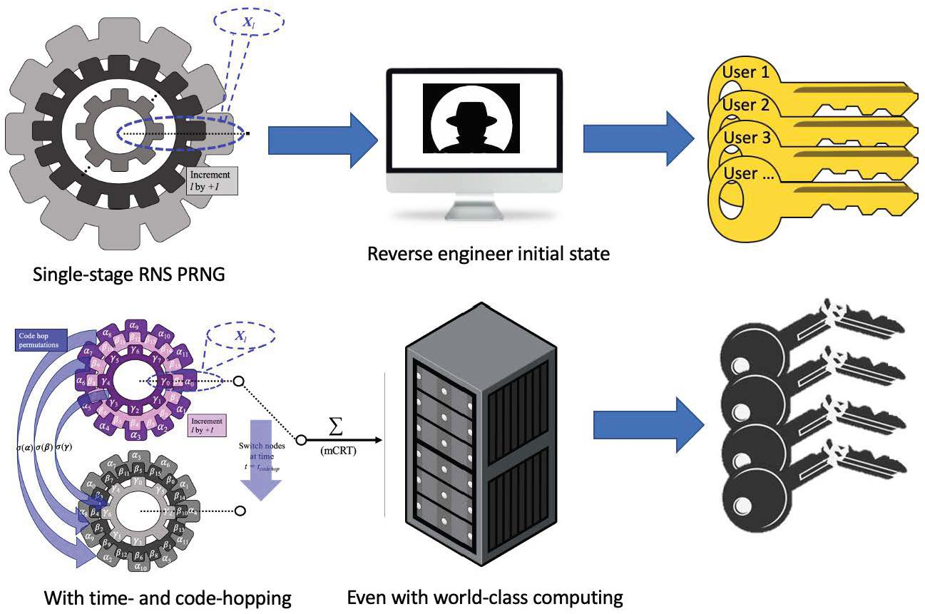
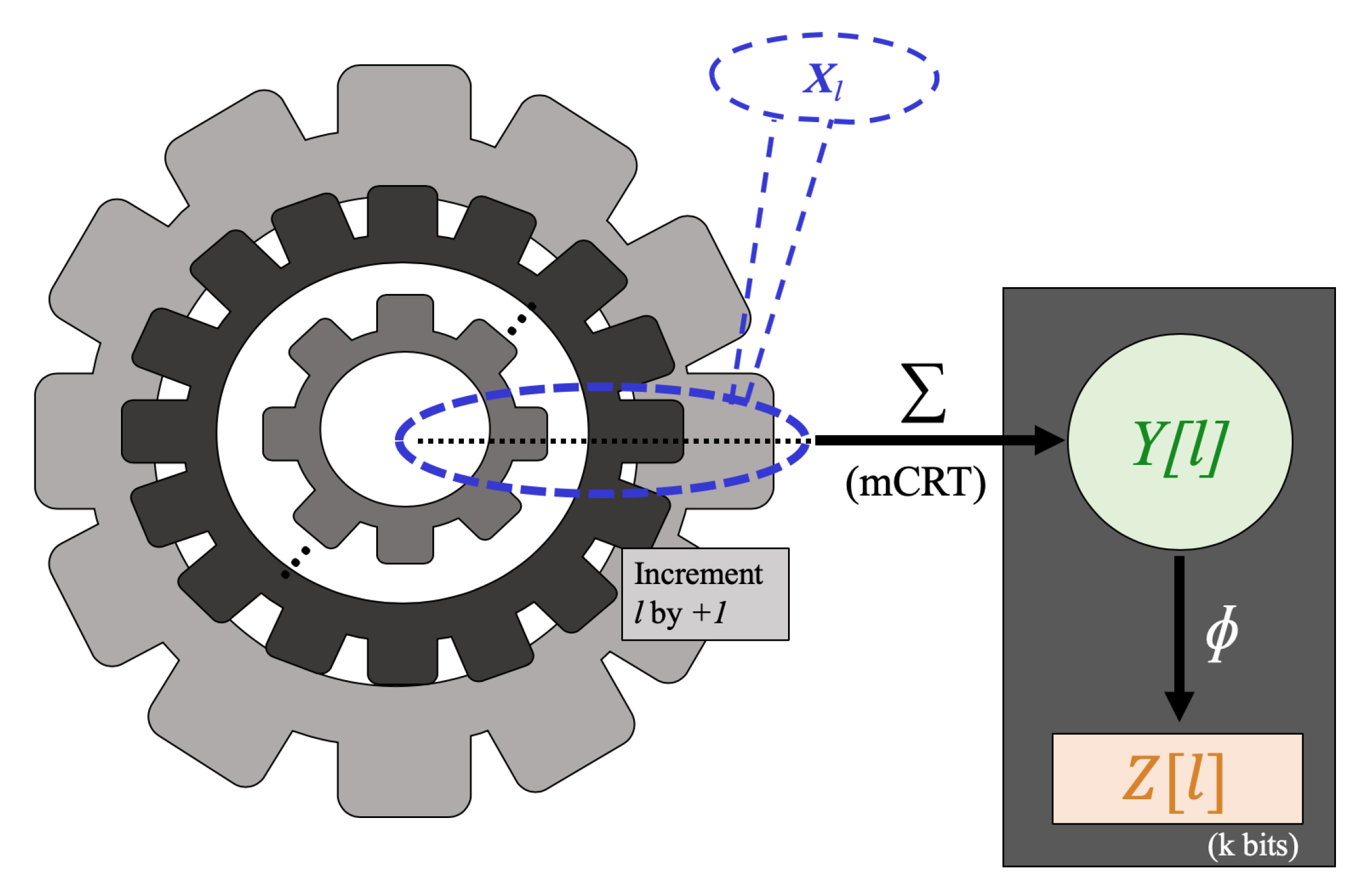
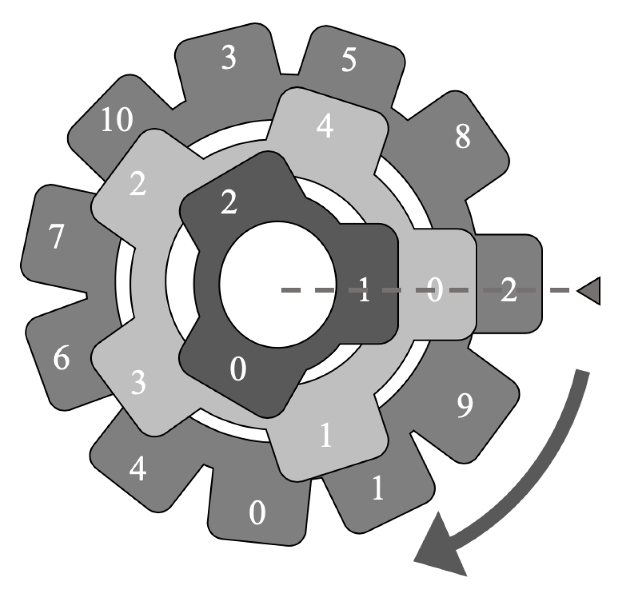
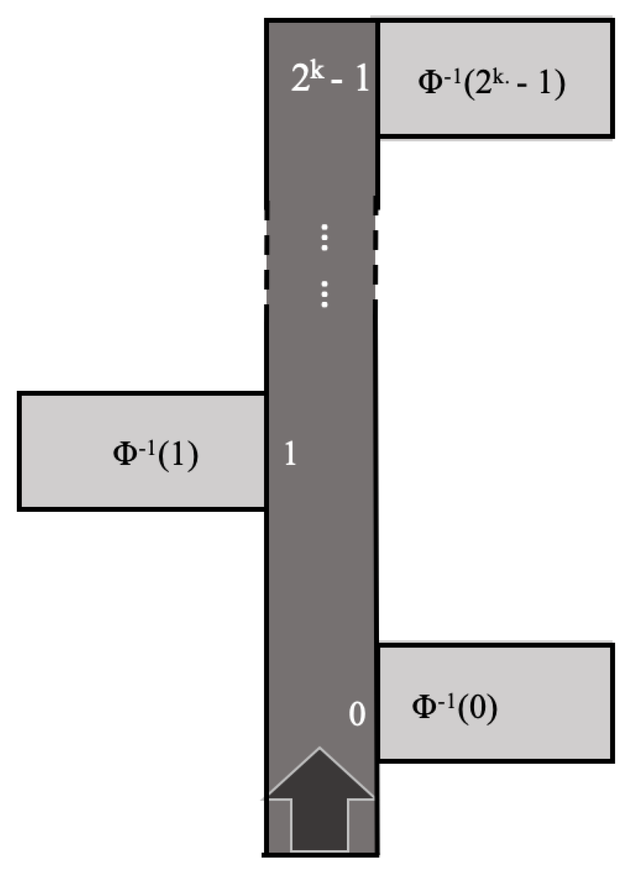
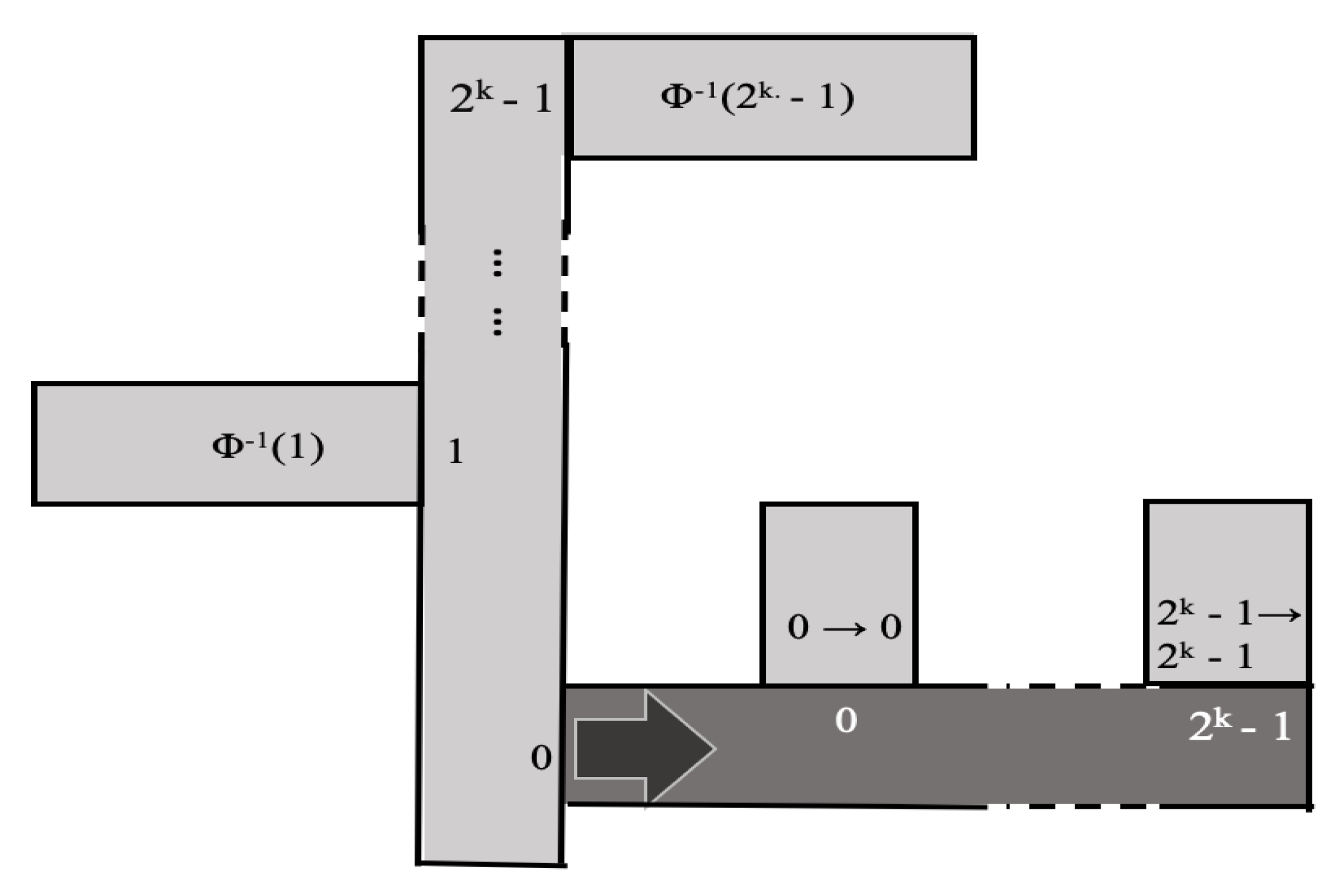
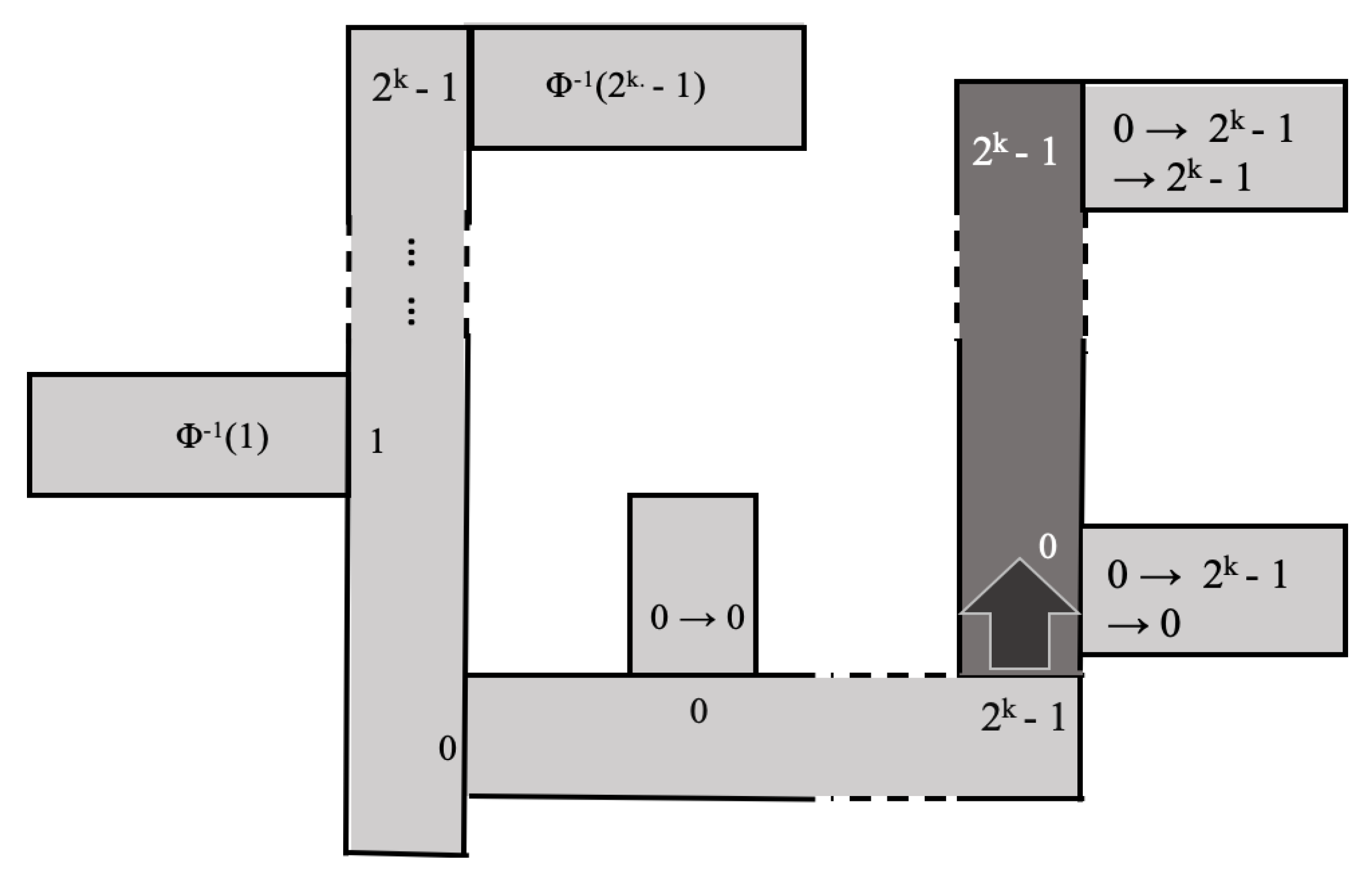
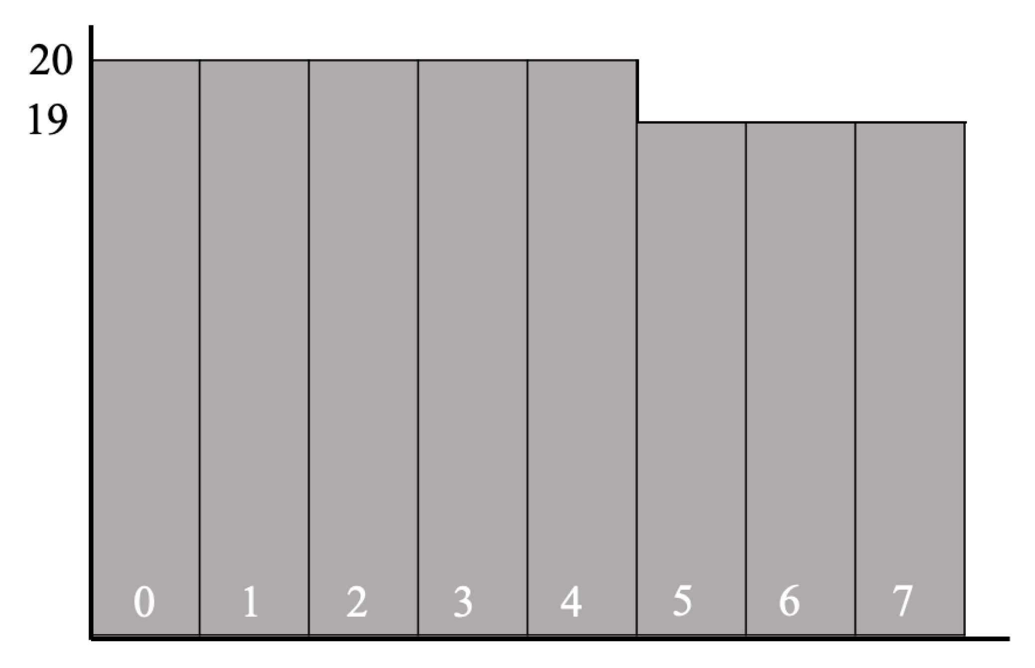
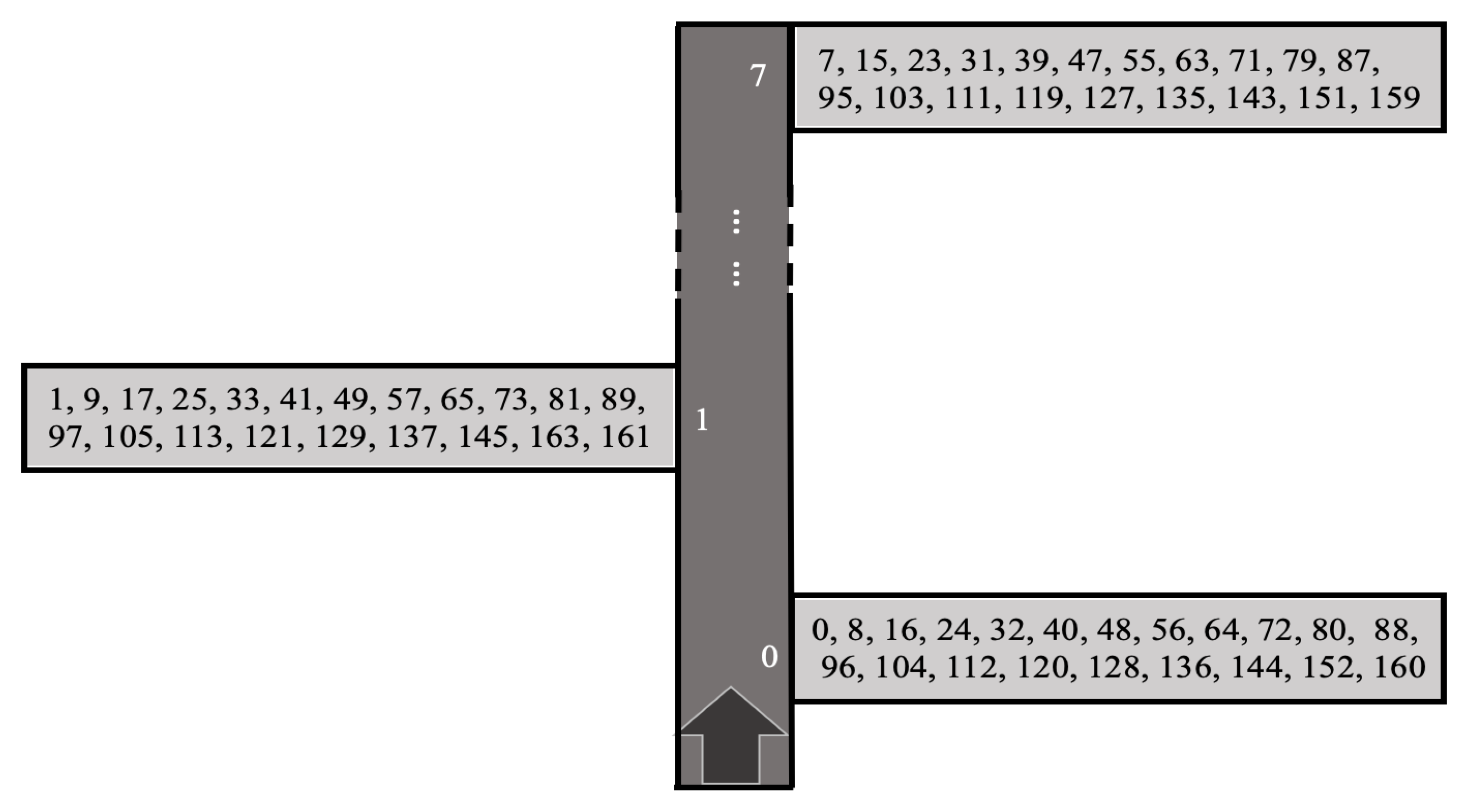
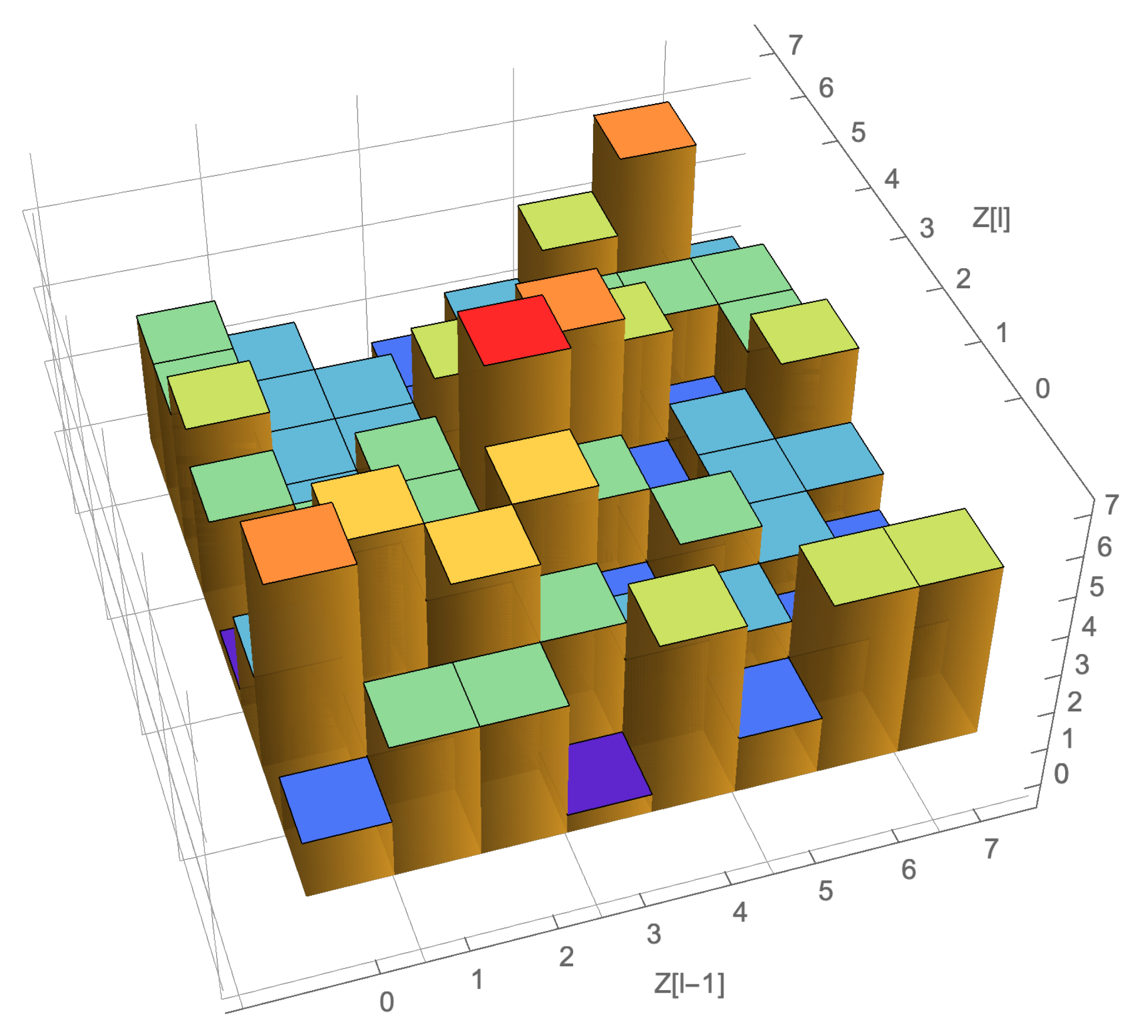
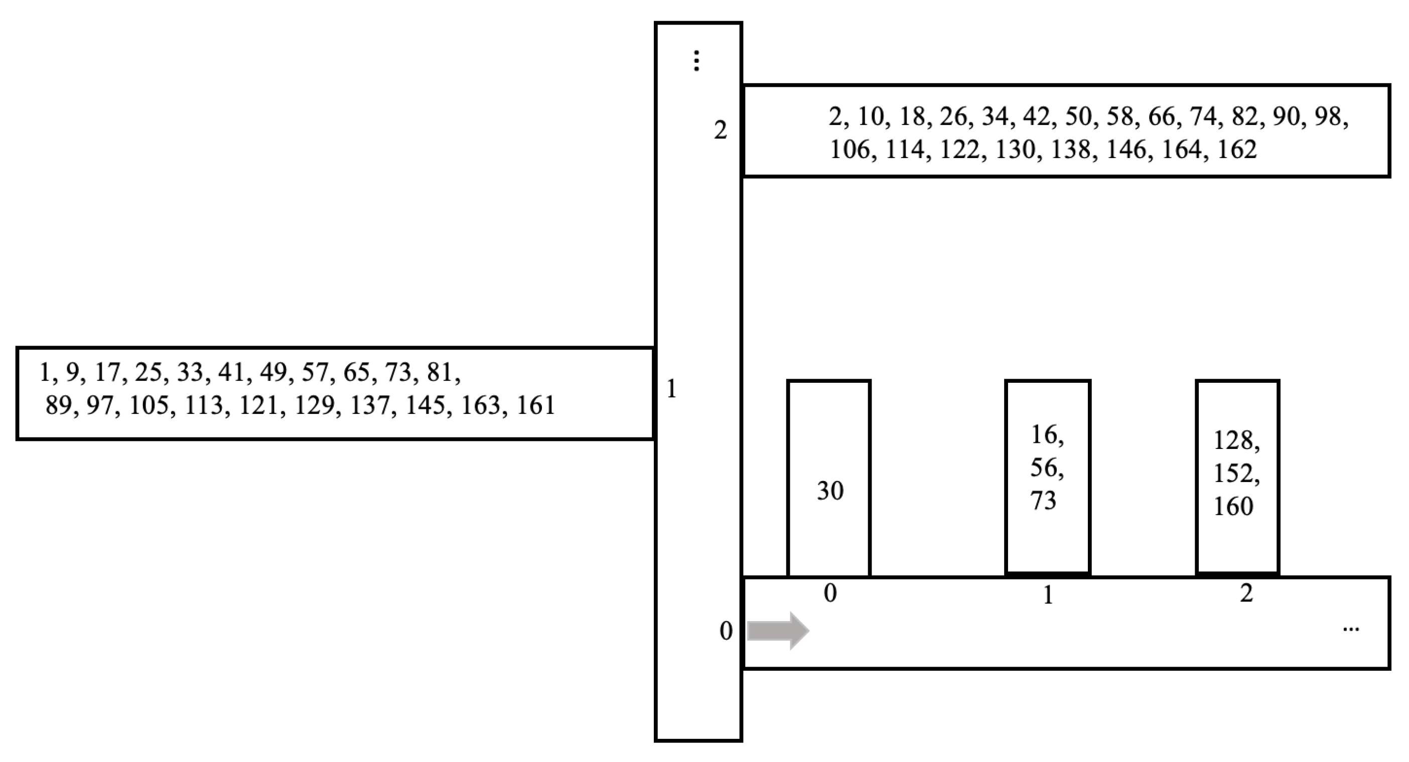
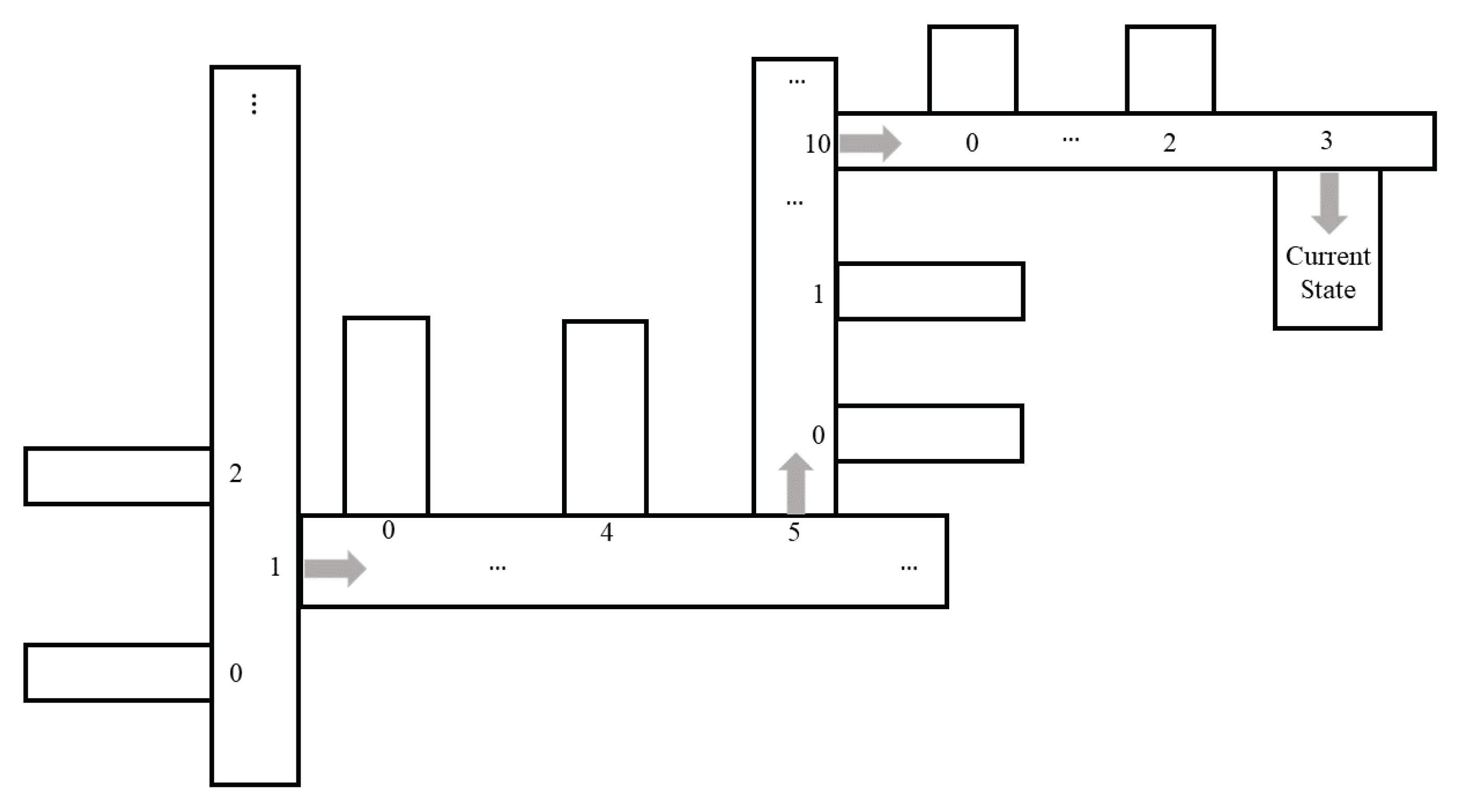
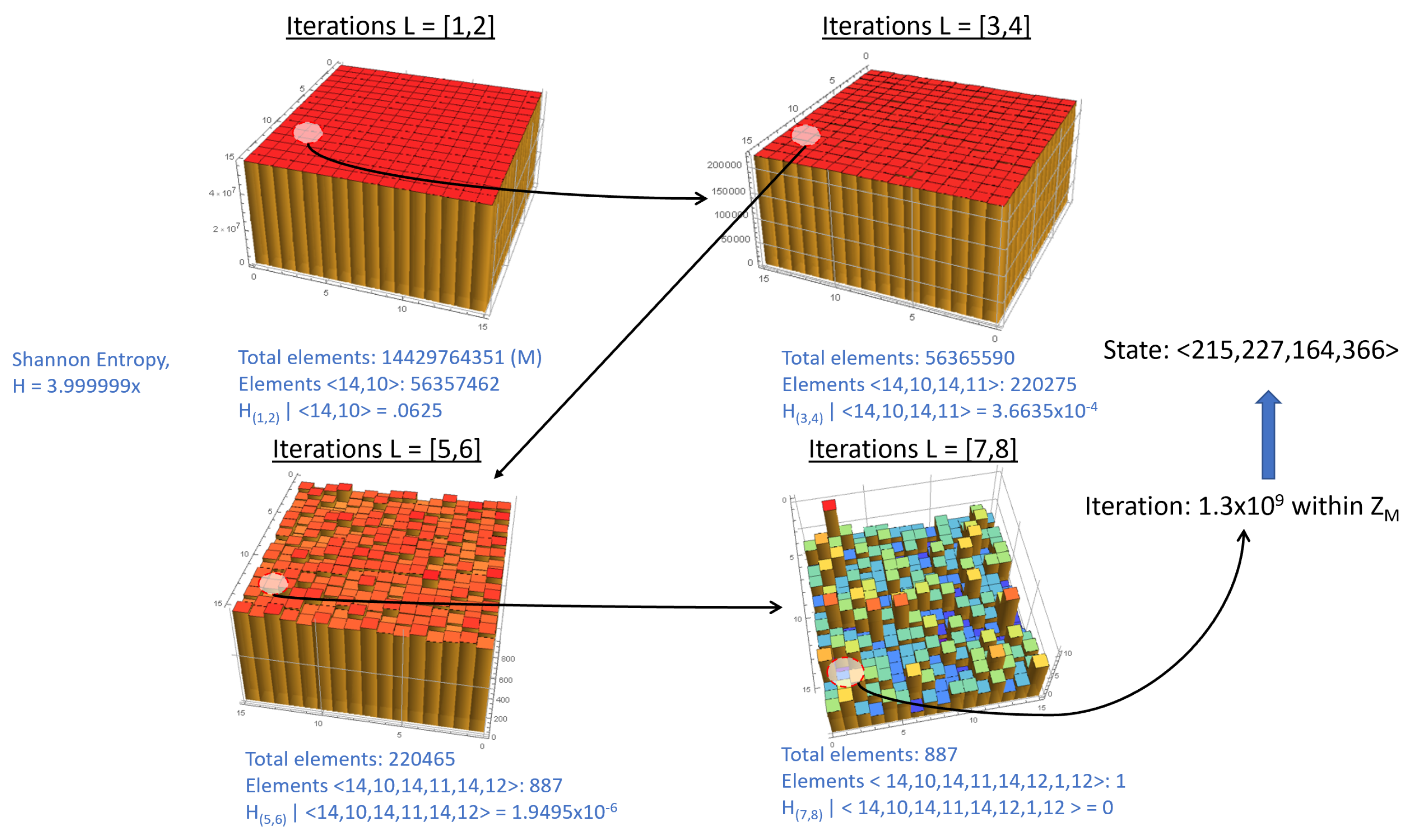
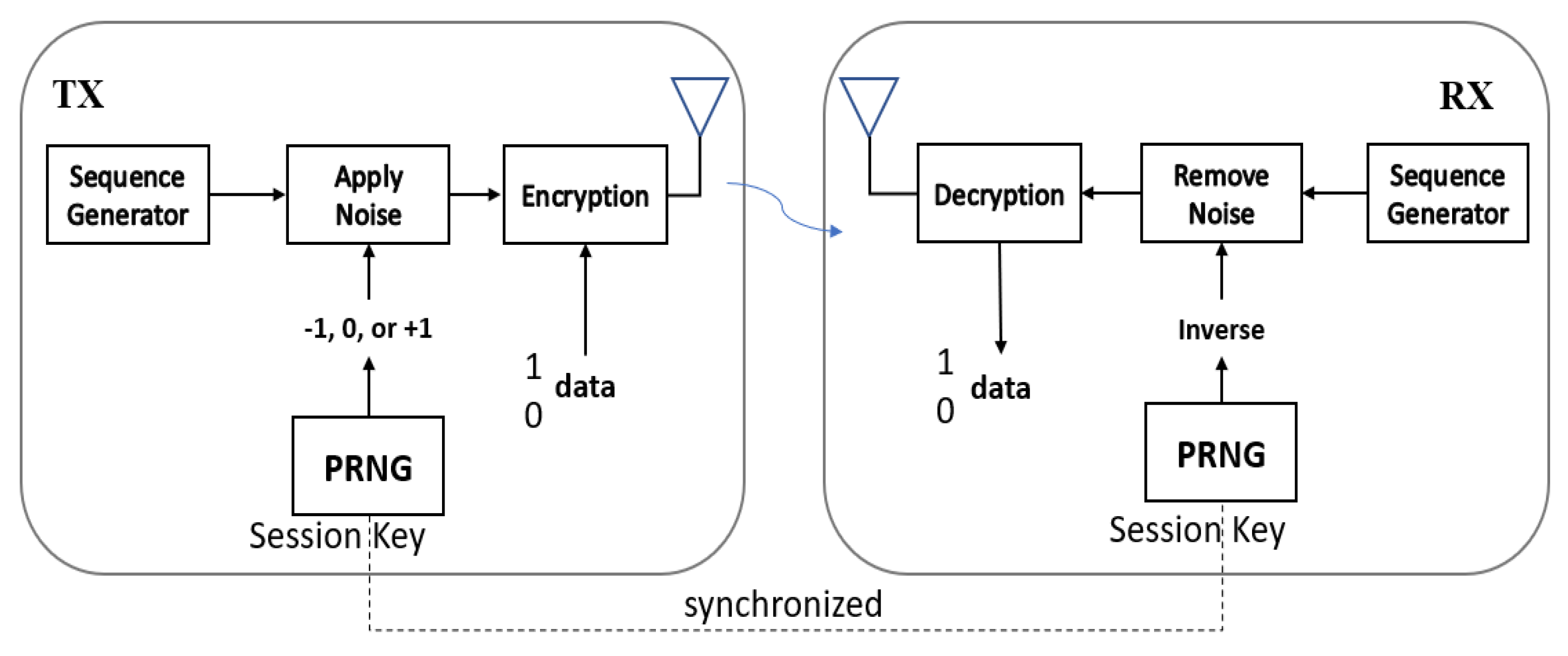
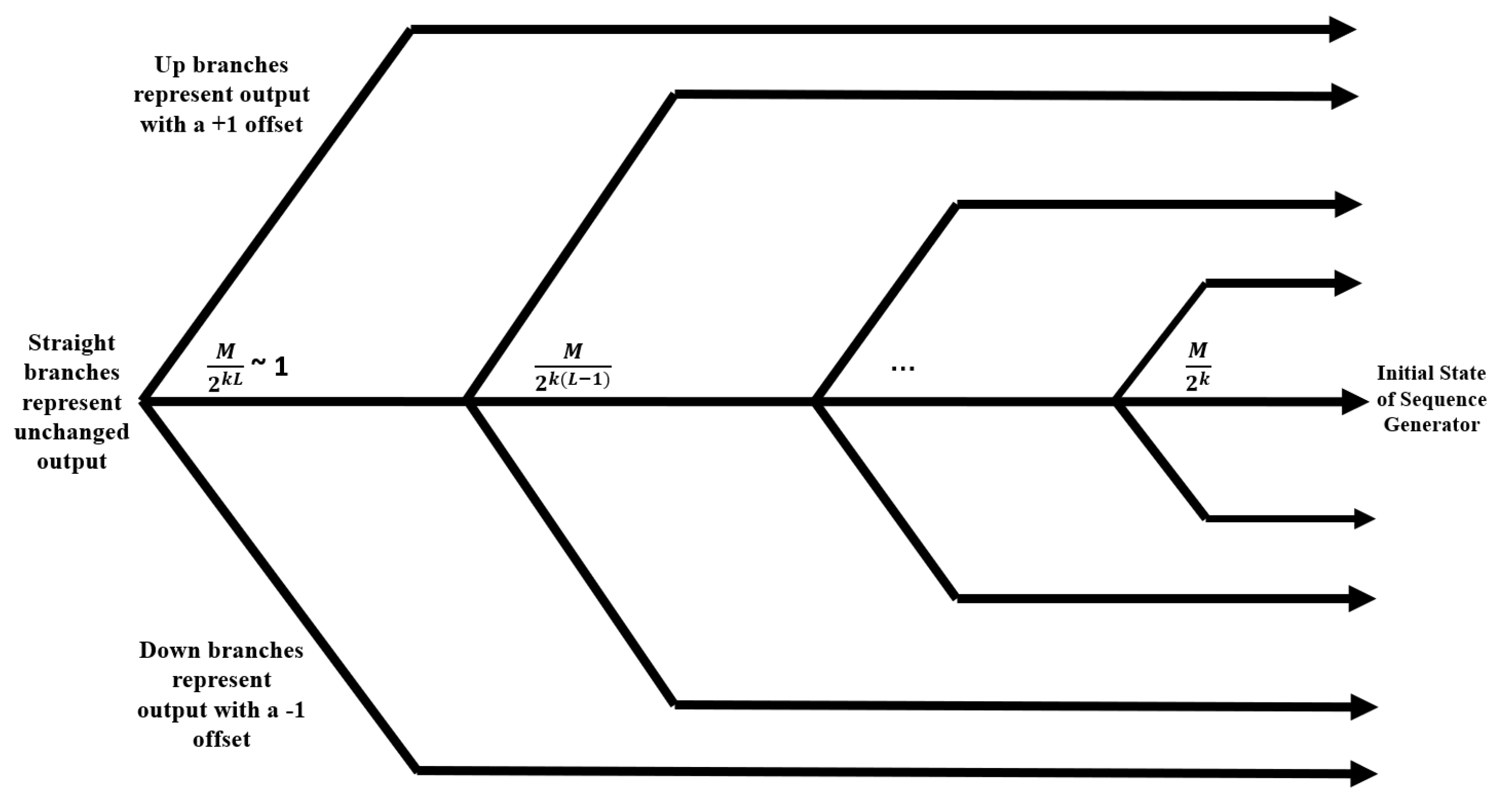
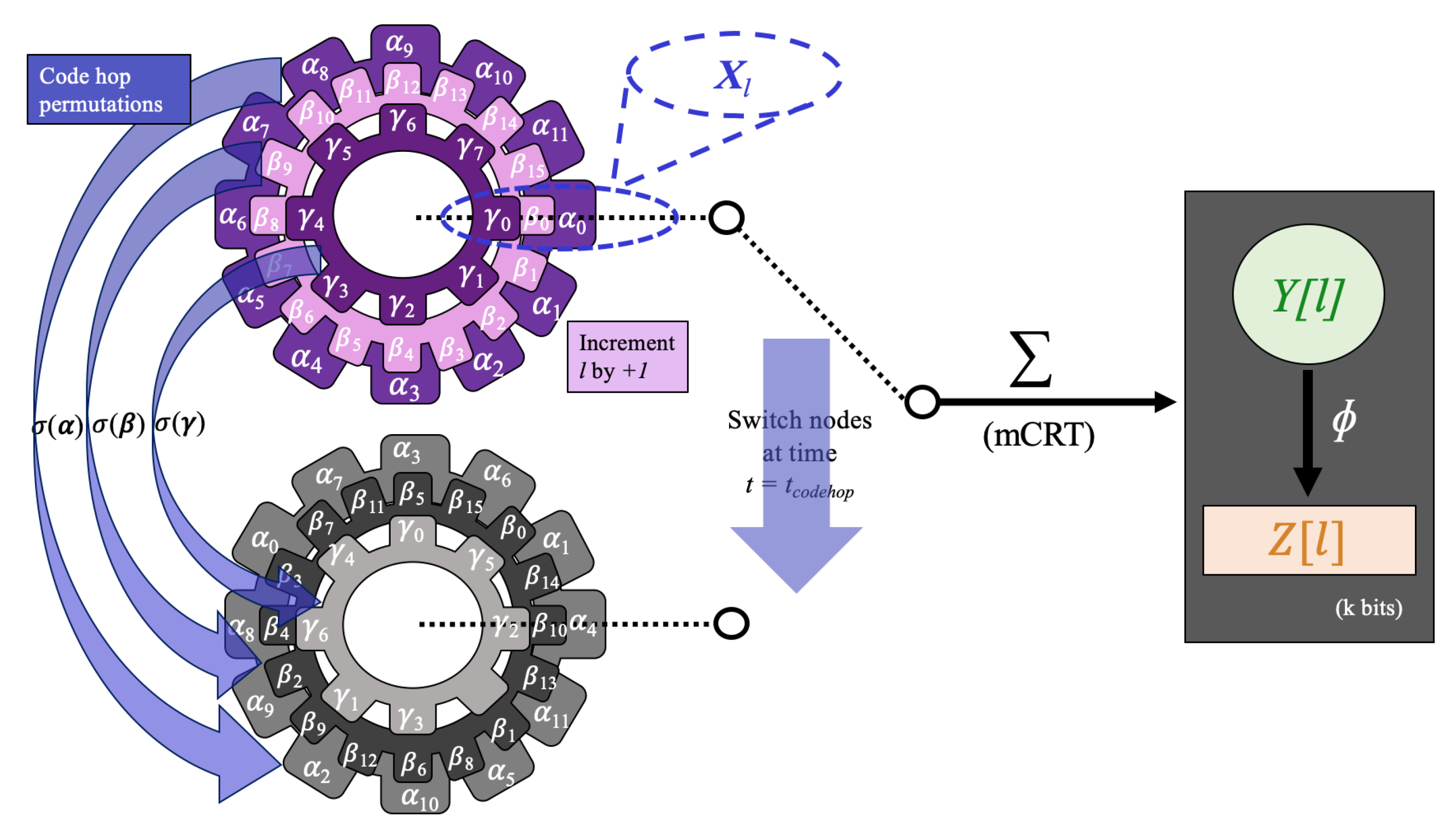
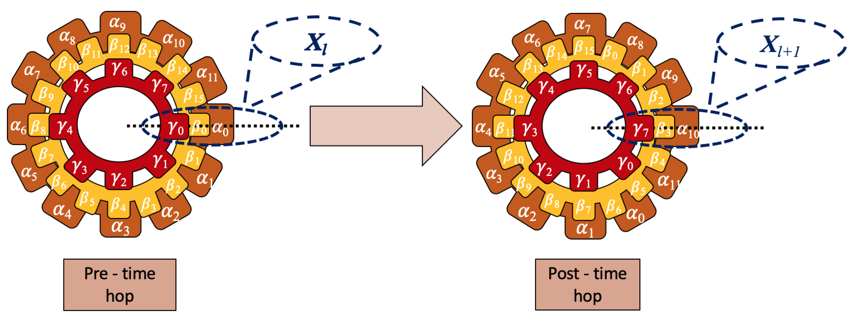
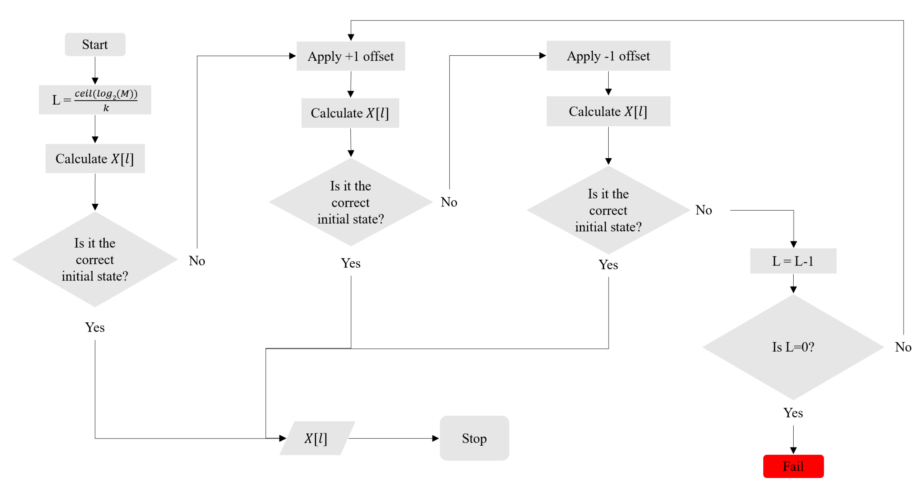
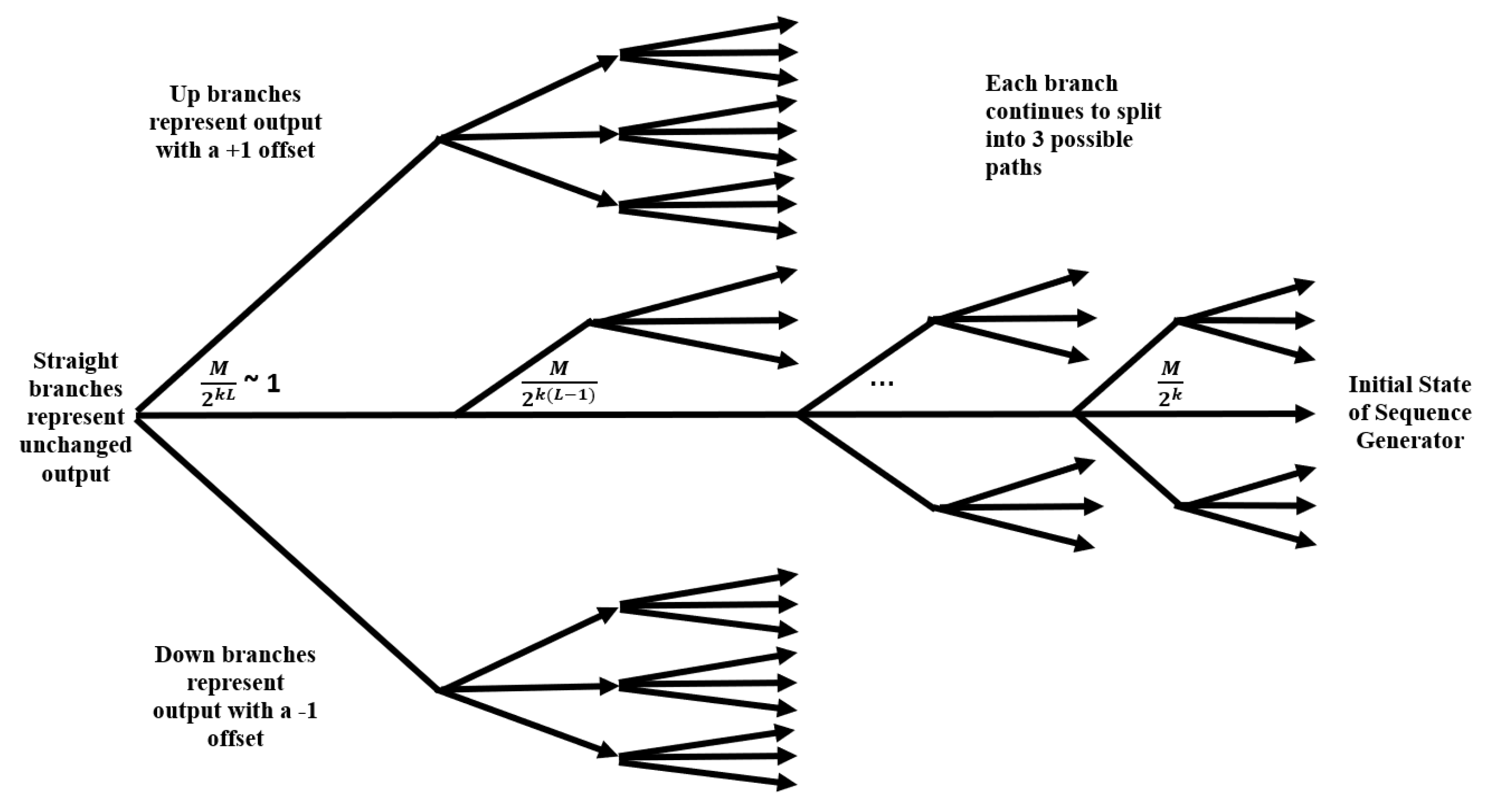
Table 1.
Descriptions of the mathematical computations in Figure 1.
Table 1.
Descriptions of the mathematical computations in Figure 1.
| Label | Description |
|---|---|
| mCRT | |
| Surjective mapping |
Table 2.
Data from the toy example.
| l | CRT Output | |||
|---|---|---|---|---|
| 0 | 145 | 85 | 5 | |
| 1 | 141 | 3 | 3 | |
| 2 | 23 | 59 | 3 | |
| ⋮ | ⋮ | ⋮ | ⋮ | ⋮ |
| 163 | 27 | 141 | 5 | |
| 164 | 74 | 32 | 0 |
Table 3.
Analysis of time and memory requirements of varying sizes of RNS.
| n | |||||
|---|---|---|---|---|---|
| 3 | 11 | 132 | 1216 | 0.1 | ≈20.2 |
| 4 | 479 | 25,893 | ≈ | ||
| 16 | 1021 | 242,038 | ≈ | ||
| 24 | 2003 | 126,229 | ≈ |
Publisher’s Note: MDPI stays neutral with regard to jurisdictional claims in published maps and institutional affiliations. |
© 2021 by the authors. Licensee MDPI, Basel, Switzerland. This article is an open access article distributed under the terms and conditions of the Creative Commons Attribution (CC BY) license (https://creativecommons.org/licenses/by/4.0/).
Share and Cite
MDPI and ACS Style
Vennos, A.; George, K.; Michaels, A. Attacks and Defenses for Single-Stage Residue Number System PRNGs. IoT 2021, 2, 375-400. https://0-doi-org.brum.beds.ac.uk/10.3390/iot2030020
AMA Style
Vennos A, George K, Michaels A. Attacks and Defenses for Single-Stage Residue Number System PRNGs. IoT. 2021; 2(3):375-400. https://0-doi-org.brum.beds.ac.uk/10.3390/iot2030020
Chicago/Turabian StyleVennos, Amy, Kiernan George, and Alan Michaels. 2021. "Attacks and Defenses for Single-Stage Residue Number System PRNGs" IoT 2, no. 3: 375-400. https://0-doi-org.brum.beds.ac.uk/10.3390/iot2030020