Robust Haebara Linking for Many Groups: Performance in the Case of Uniform DIF

Abstract

The comparison of group means in item response models constitutes an important issue in empirical research. The present article discusses a slight extension of the robust Haebara linking approach of He and Cui by proposing a flexible class of robust Haebara linking functions for comparisons of many groups. These robust linking functions are robust against violations of invariance. In this article, we investigate the performance of robust Haebara linking in the presence of uniform DIF effects. In an analytical derivation, it is shown that the robust Haebara linking approach provides unbiased estimates of group means in the limiting case $p=0$. In a simulation study, it is demonstrated that the proposed variant of the Haebara linking approach outperforms existing implementations of Haebara linking to some extent. In an empirical application using PISA data, it is illustrated that country means can be sensitive to the choice of linking functions.

1. Introduction

One primary goal of empirical studies in psychology and education is to compare cognitive outcomes across many groups. For example, the programme for international student assessment (PISA; [1]) provides international comparisons of student performance for a large group of countries (72 countries in PISA 2015). A major obstacle to these comparisons is that cognitive tests often show differential item functioning (DIF; [2]).

In this article, we investigate robust variants to the originally proposed Haebara linking method [3] for many groups. We study a slight extension of robust Haebara linking that was proposed by He and Cui [4] by using a more flexible class of loss functions. We use a two-parameter logistic model (2PL) item response model to introduce the methodology. It is shown that approximately unbiased group comparisons can be conducted with robust Haebara linking when group-specific subsets of items show DIF (i.e., partial invariance). Importantly, no additional steps for identifying items with DIF are needed; items that possess DIF are essentially treated as outliers [5,6] in the linking procedure.

The paper is structured as follows. Section 2 describes the 2PL model under partial invariance that allows the presence of uniform DIF effects. Section 3 introduces the robust Haebara linking method. It is argued that the proposed linking method can provide unbiased estimates in the presence of uniform DIF. In Section 4, the proposed method is evaluated in a simulation study. Section 5 presents an empirical example of PISA data. Finally, Section 6 concludes with a discussion that focuses on limitations and potential gaps for future research.

2. 2PL Model with Partial Invariance: Presence of Uniform DIF Effects

In the following, we introduce the concept of partial invariance for multiple groups. For G groups $(g=1,\dots ,G)$, I items $(i=1,\dots ,I)$ are administered. It is assumed that a unidimensional item response model holds in each group with group-specific item response functions (IRF) $P_{ig}(\theta )$, indicating the probability of a correct item response $X_{ig}$, conditional on ability $\theta$. The IRFs in the 2PL model [7] are given as

$$P(X_{ig}=1|{\theta }_g)=\mathrm{\Psi }(a_{ig}({\theta }_g-b_{ig})),{\theta }_g\sim N({\mu }_g,{\sigma }_g^2)$$

(1)

where $b_{ig}$ are group-specific item difficulties for item i$(i=1,\dots ,I)$ in group g ($g=1,\dots ,G$), and $a_{ig}$ are group-specific item loadings. In this article, we focus on the case of uniform DIF [2] that presupposes that item loadings are invariant across groups, i.e., $a_{i1}=\dots =a_{iG}\equiv a_i$. Group-specific item difficulties are decomposed into $b_{ig}=b_i+e_{ig}$, where $b_i$ indicates common item difficulties and $e_{ig}$ are denoted as uniform DIF effects. In Equation (1), $\mathrm{\Psi }$ denotes the logistic distribution function, and it is assumed that the abilities within each group g are normally distributed with mean ${\mu }_g$ and standard deviation ${\sigma }_g$.

It is well known that not all DIF effects $e_{ig}$ and group means ${\mu }_g$ can be simultaneously identified in the 2PL model [8,9]. To resolve the identification issue, the set of items for each group is partitioned into two distinct sets (see [10]). More specifically, we assume that for each group g, a subset of so-called anchor items ${\mathcal{J}}_{A,g}\subset \mathcal{J}=\{1,\dots ,I\}$ exists such that $e_{ig}=0$ for all $i\in {\mathcal{J}}_{A,g}$. The set of biased items is defined as ${\mathcal{J}}_{B,g}=\mathcal{J}\backslash {\mathcal{J}}_{A,g}$. Biased items are allowed to possess DIF effects $e_{ig}\ne 0$, which differs from zero. This situation is also referred to in the literature as partial invariance [11,12]. If there are no biased items, all item parameters are invariant, which is denoted as full invariance. One central argument in the DIF literature is that items with DIF effects have the potential to bias the estimated ability distributions (i.e., group means or group standard deviations) and should, therefore, not be included in group comparisons (e.g., [1], for arguments in the PISA study, or [13]). Biased estimates of group means can be particularly expected in the case that all DIF effects of items within a group have the same sign (i.e., unbalanced DIF).

In practice, it is not known which items serve as anchor items for group g. The choice can be based on a substantive basis (e.g., considerations outside of psychometrics, see [14]) or using psychometric methods. In this article, the identification of group means and group standard deviations is conducted using psychometric methods, namely linking methods (see [15,16,17,18,19] for overviews). Linking methods rely on separate scalings for all groups. In more detail, the 2PL model is fitted for each group (under the assumption $\theta \sim N(0,1)$), resulting in estimated item loadings ${\widehat{\mathit{a}}}_g$ and estimated item intercepts ${\widehat{\mathit{b}}}_g$ for all groups. In the second step, estimated parameters $({\widehat{\mathit{a}}}_g,{\widehat{\mathit{b}}}_g)$ are used to determine the vector of group means $\mathbf{\mu }=({\mu }_1,\dots ,{\mu }_G)$ and $\mathbf{\sigma }=({\sigma }_1,\dots ,{\sigma }_G)$ standard deviations.

Alternatively, biased items could be determined by a statistical DIF detecting method prior to linking (see, e.g., [12,20,21]). The linking method is then subsequently applied only on the anchor items. This approach relies on the somewhat arbitrary choice of a cutoff value for the DIF statistic. In this article, the proposed robust Haebara linking method does not require a prior determination of biased items, and in the next section, it is shown it can provide unbiased group mean estimates in the case of uniform DIF effects.

3. Haebara Linking

In this section, we introduce the robust Haebara linking method that determines group means $\mathbf{\mu }$, group standard deviations $\mathbf{\sigma }$, common item slopes $\mathit{a}=(a_1,\dots ,a_I)$, and common item difficulties $\mathit{b}=(b_1,\dots ,b_I)$ based on estimated item loadings ${\widehat{\mathit{a}}}_g$ and estimated item intercepts ${\widehat{\mathit{b}}}_g$ for all groups g. A linking function H is employed that minimizes the distances between group-specific IRFs and aligned common IRFs for computing unknown parameters $(\mathbf{\mu },\mathbf{\sigma },\mathit{a},\mathit{b})$

$$H(\mathbf{\mu },\mathbf{\sigma },\mathit{a},\mathit{b})={\displaystyle \sum _{i=1}^I}{\displaystyle \sum _{g=1}^G}\int \rho \left(\mathrm{\Psi }({\widehat{a}}_{ig}[\theta -{\widehat{b}}_{ig}])-\mathrm{\Psi }(a_i[{\sigma }_g\theta -b_i+{\mu }_g])\right)\omega (\theta )\mathrm{d}\theta$$

(2)

where $\rho$ is a loss function, and $\omega$ is a weighting function that fulfills $\int \omega (\theta )\mathrm{d}\theta =1$. In all subsequent analyses, we choose the standard normal density function as the weighting function $\omega$. Linking based on the function H in Equation (2) is referred to as robust Haebara linking and generalizes the originally proposed Haebara linking method for two groups [3] that uses the loss function $\rho (x)=x^2$. He and colleagues [4,22] considered the loss function $\rho (x)=\left|x\right|$ for two groups. Haebara linking for multiple groups was investigated in several articles [10,23,24,25]. In particular, it was shown in [10] that the loss function $\rho (x)=\left|x\right|$ was efficient in handling the situation of partial invariance for multiple groups.

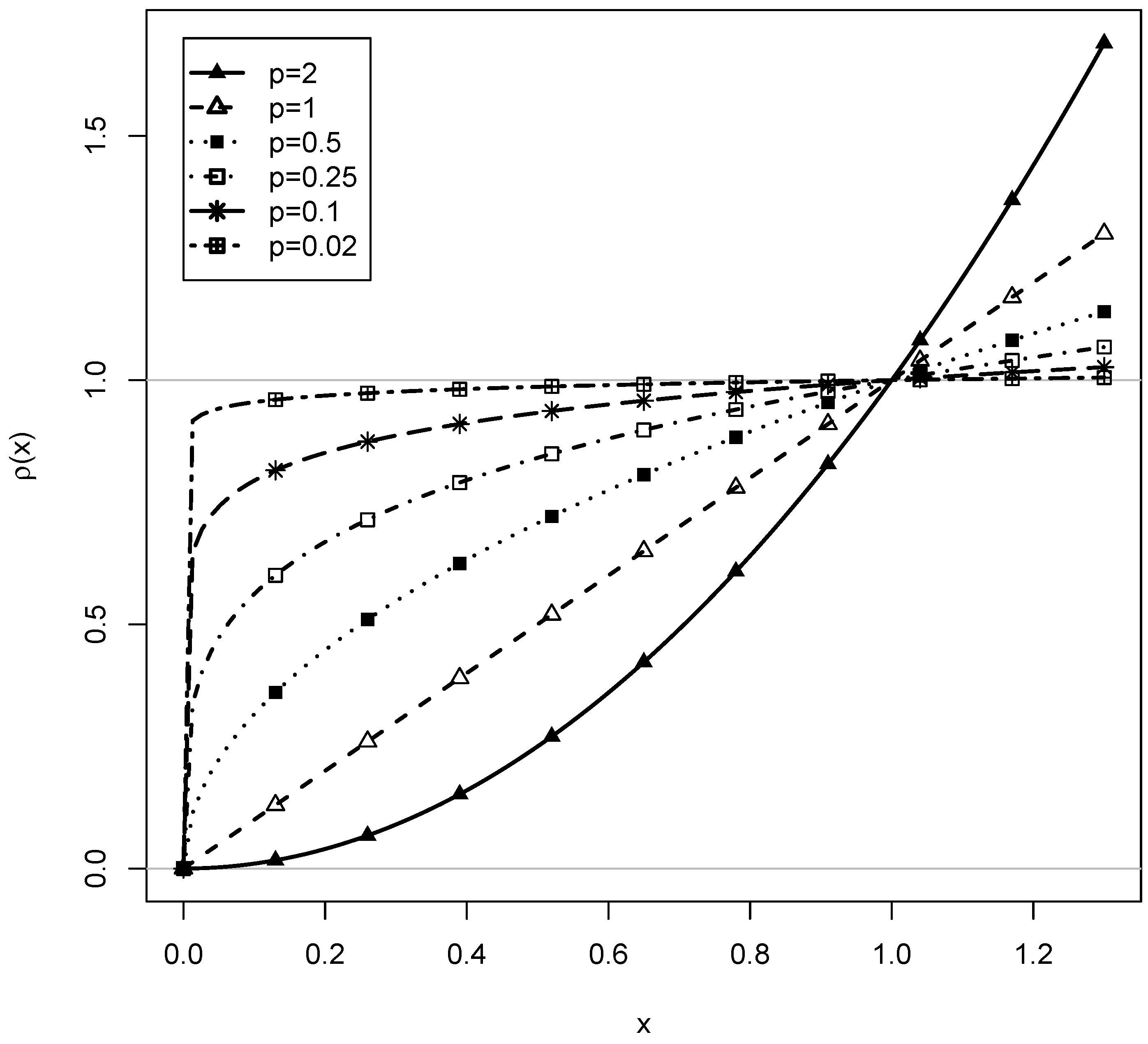
In this article, we consider the class of loss function $\rho (x)={\left|x\right|}^p$ with nonnegative power values p. In Figure 1, the loss functions for different values of p are shown. It can be seen that $p=1$ and $p=2$ put different weights for values near zero. In the limiting case of $p\to 0$, $\rho (x)$ is the step function that takes the value 0 if x is zero, and 1 for all other x values. With $\rho (x)={\left|x\right|}^p$ for very small p values (e.g., $p=0.02$) in Equation (2), the linking function essentially counts the number of events in which the group-specific IRF deviates from the aligned common IRF.

It should be noted that there are competitive linking methods to Haebara linking. The Stocking-Lord method [26] minimizes the difference of the integrated squared difference of the sum of group-specific IRFs and the sum of aligned common IRFs. There are also alternative linking approaches that directly rely on estimated item parameters instead of IRFs, such as mean-mean linking [17], Haberman linking based on regression modeling [27], invariance alignment [28], and distance-based measures (like ${\chi }^2$; [29,30]), to name a few. For Haberman linking and invariance alignment, robust alternatives were recently studied [10,31,32,33]. The linking approach is a two-step method as separate scalings are applied group-wise in the first step. However, it can be shown that one can reformulate the two-step estimation problem as a one-step estimation problem with side conditions [34].

3.1. Estimation

In the minimization of the robust Haebara linking function H defined in Equation (2), the unknown parameters can be obtained by setting the first derivatives to 0, i.e., $\frac{\partial H}{\partial \mathbf{\mu }}=0$, $\frac{\partial H}{\partial \mathbf{\sigma }}=0$, $\frac{\partial H}{\partial \mathit{a}}=0$, and $\frac{\partial H}{\partial \mathit{b}}=0$. However, the loss function $\rho (x)={\left|x\right|}^p$ is not differentiable for $p\le 1$, and the first derivative must be replaced by a subdifferential. Moreover, due to nondifferentiability of $\rho$, standard optimization algorithms that rely on derivatives cannot be used. However, in robust Haebara linking, the function $\rho (x)={\left|x\right|}^p$ is replaced by a differentiable approximating function ${\rho }_D(x)={(x^2+\epsilon )}^{p/2}$ using a small $\epsilon >0$ (e.g., $\epsilon =0.001$). Because ${\rho }_D$ is differentiable, quasi-Newton minimization approaches can be used that are implemented in standard optimizers in R [35]. The implementation of robust Haebara linking in the sirt [36] package specifies a sequence of decreasing values of $\epsilon$ in the optimization, each using the previous solution as initial values (see [37] for a similar approach). It should be noted that alternative differentiable approximating function for the loss function $\rho (x)={\left|x\right|}^p$ for values p nearby zero have been employed [38].

3.2. Estimated Group Means as a Function of DIF Effects

Next, we investigate the bias in estimated group means of robust Haebara linking for infinite sample sizes (i.e., the asymptotic bias). Assume that the vector of joint item parameters $\mathit{a}$ and $\mathit{b}$ and group standard deviations $\mathbf{\sigma }$ are already identified. We now investigate the estimated group mean ${\widehat{\mu }}_g$ and use the part in Equation (2) that relates to the group mean ${\mu }_g$. The estimate ${\widehat{\mu }}_g$ can be determined as

$${\widehat{\mu }}_g=\underset{\mu }{arg\; min}\left\{{\displaystyle \sum _{i=1}^I}\int \rho \left(\mathrm{\Psi }({\widehat{a}}_{ig}[\theta -{\widehat{b}}_{ig}])-\mathrm{\Psi }(a_i[{\sigma }_g\theta -b_i+\mu ])\right)\omega (\theta )\mathrm{d}\theta \right\}$$

(3)

By using two Taylor approximations, we can formulate the estimated group mean ${\widehat{\mu }}_g$ as a function of the true mean ${\mu }_g$ and weighted DIF effects $e_{ig}$. For $p\ne 1$, we get (see Appendix A; Equation (A11))

$${\widehat{\mu }}_g={\mu }_g-\frac{1}{p-1}\frac{{\displaystyle {\displaystyle \sum _{i=1}^I}{w}_{ig}{e}_{ig}}}{{\displaystyle {\displaystyle \sum _{i=1}^I}{w}_{ig}}}$$

(4)

where $w_{ig}={\left|e_{ig}\right|}^{p-2}\int W_i{(\theta )}^p\omega (\theta )\mathrm{d}\theta$, and $W_i$ is the information function of item i. The item-specific weights $w_{ig}$ consist of two factors. First, the factor $|e_{ig}{|}^{p-2}$ governs the influence of DIF effects. Items with large DIF effects $e_{ig}$ are down-weighted for $p<2$. Second, the factor $\int W_i{(\theta )}^p\omega (\theta )\mathrm{d}\theta$ is the integrated information function with respect to $\omega$. The influence of this factor is largest for items with large item loadings $a_i$ and item difficulties $b_i$ that are located in the center of the ability distribution.

We now consider two important special cases of Equation (4). For $p=2$, we obtain the Haebara linking proposed in [3], and it holds that

$${\widehat{\mu }}_g={\mu }_g-\frac{{\displaystyle {\displaystyle \sum _{i=1}^I}\left(\int W_i(\theta )\omega (\theta )\mathrm{d}\theta \right)e_{ig}}}{{\displaystyle {\displaystyle \sum _{i=1}^I}\int W_i(\theta )\omega (\theta )\mathrm{d}\theta }}$$

(5)

All DIF effects are weighted according to their item information function. There is no down-weighting of large DIF effects because the weights only involve the integrated information functions. In the case of $p=1$ (as proposed in [4,22]), it can be shown that the bias in estimated group means in robust Haebara linking is a weighted median of DIF effects (see Equation (A15) in Appendix A.5 and [39]).

Finally, it is shown in Appendix A.6 that the estimated group means can be estimated without an asymptotic bias in the limiting case that p equals 0. For $p=0$, within each group, the linking function H counts the number of items that show DIF. Hence, the number of noninvariant items is minimized within each group. The minimum within each group is given as $|{\mathcal{J}}_{B,g}|$, i.e., the number of biased items within each group. In empirical applications of robust Haebara linking it can be expected that the bias decreases with decreasing values of p. Obviously, the reasoning relies on asymptotic arguments, and it is of interest whether the property also holds true in moderately sized samples and to assess a potential loss of efficiency in using small values of p in applications.

4. Simulation Study

In this simulation study, we investigate the statistical properties of the proposed robust Haebara linking method in the presence of uniform DIF effects. The primary goal is to assess the performance of group mean estimates in terms of bias and variability.

4.1. Simulation Design

In this study, we generated dichotomous item responses and investigated the performance of robust Haebara linking for the 2PL model. We simulated item responses from a 2PL model for $G=9$ groups. For each group g, abilities were normally distributed with mean ${\mu }_g$ and standard deviation ${\sigma }_g$. Across all conditions and replications of the simulation, the group means and standard deviations were held fixed (see Appendix B for values used in the simulation). The total population comprising all groups had a mean of 0 and a standard deviation of 1.

Item responses $X_{ig}$ for item i in group g were simulated according to the 2PL model

$$P(X_{ig}=1|{\theta }_g)=\mathrm{\Psi }(a_i({\theta }_g-b_i-Z_{ig}\delta ))$$

(6)

where DIF effects in item difficulties were defined as $e_{ig}=Z_{ig}\delta$. The DIF indicator variables $Z_{ig}$ had values of 0, 1, or $-1$, where values different from zero indicated uniform DIF effects. For each country, either all nonzero $Z_{ig}$ values were 1 or were $-1$, meaning that all DIF effects had the same direction (i.e., unbalanced DIF). Item loadings $a_i$ were assumed to be invariant across groups. The DIF effect size was chosen as $\delta =0.6$, and it resembles moderate to high amounts of DIF [40,41]. A fixed proportion ${\pi }_B$ of biased items was selected and was equal across groups, i.e., ${\sum }_{i=1}^I\left|Z_{ig}\right|=I{\pi }_B$ for all groups $g=1,\dots ,G$. For example, if $30\%$ out of $I=20$ items have DIF effects, 6 items have values of $Z_{ig}$ that differ from zero. The item parameters were held constant across conditions and replications (see Appendix B for data-generating parameters). In total, $I=20$ items were used in the simulation.

For each condition of the simulation design, a relatively low number $R=300$ replicated datasets was used because we were only interested in statistical properties of point estimates. We manipulated the number of persons per group ($N=250$, 500, 1000, and 5000) to cover situations of small-scale and large-scale studies. The case of $N=5000$ persons per group corresponds to the situation in which identified item parameters are estimated with negligible sampling errors. We also varied the proportion ${\pi }_B$ of biased items with DIF effects (0, 10, and $30\%$).

4.2. Analysis Methods

The performance of robust Haebara linking with powers $p=2$, 1, 0.5, 0.25, 0.1, and 0.02 for estimated group means were compared with the scaling approach that relies on full invariance of all item parameters. The approach with full invariance (FI) was specified as a 2PL multiple group item response model.

To identify group means and group standard deviations in the linking procedure, for the first group, the mean was set to 0, and the standard deviation was set to 1. Estimated group means and group standard deviations were linearly transformed to obtain a mean of 0 and a standard deviation 1 for the total sample comprising all groups. These conditions were also fulfilled in the data generating model (see Section 4.1).

The statistical performance of the vector of estimated means $\widehat{\mathbf{\mu }}$ is assessed by summarizing the biases and variances of estimators across groups. Let $\mathbf{\mu }=({\mu }_1,\dots ,{\mu }_G)$ be a parameter of interest and $\widehat{\mathbf{\mu }}=({\widehat{\mu }}_1,\dots ,{\widehat{\mu }}_G)$ its estimator (i.e., for means and standard deviations). For R replications, the obtained estimates are ${\widehat{\mathbf{\mu }}}_r=({\widehat{\mu }}_{1r},\dots ,{\widehat{\mu }}_{Gr})$ ($r=1,\dots ,R)$. The average absolute bias (ABIAS) is defined as

$$ABIAS(\widehat{\mathbf{\mu }})=\frac{1}{G}{\displaystyle \sum _{g=1}^G}\left|\frac{1}{R}{\displaystyle \sum _{r=1}^R}{\widehat{\mu }}_{gr}-{\mu }_g\right|=\frac{1}{G}{\displaystyle \sum _{g=1}^G}\left|Bias({\widehat{\mu }}_g)\right|$$

(7)

The average root mean square error (ARMSE) is computed as the average of the root mean square error (RMSE) of all group means:

$$ARMSE(\widehat{\mathbf{\mu }})=\frac{1}{G}{\displaystyle \sum _{g=1}^G}\sqrt{\frac{1}{R}{\displaystyle \sum _{r=1}^R}{\left({\widehat{\mu }}_{gr}-{\mu }_g\right)}^2}=\frac{1}{G}{\displaystyle \sum _{g=1}^G}RMSE({\widehat{\mu }}_g)$$

(8)

The simulation uncertainty for the ABIAS and ARMSE criteria is summarized by Monte Carlo standard errors (MCSE; see [42]). As suggested by an anonymous reviewer, bootstrap samples of replicated values are drawn, and the standard deviation of the ABIAS and ARMSE values across bootstrap samples served as estimates of the MCSE.

In all analyses, the statistical software R [35] was used. Robust Haebara linking was carried out with the sirt::linking.haebara() function in the R package sirt [36]. The TAM::tam.mml.2pl() function in the R package TAM [43] was used for estimating the 2PL model with marginal maximum likelihood as the estimation method.

4.3. Results

In

Table 1. Average Absolute Bias (ABIAS) and Average Root Mean Square Error (ARMSE) of Group Means as a Function of Sample Size.

		ABIAS				ARMSE
Model	$N$	250	500	1000	5000	250	500	1000	5000
FI		$0.006$	$0.001$	$0.003$	$0.001$	$0.059$	$0.042$	$0.029$	$0.013$
$p=2$		$0.008$	$0.002$	$0.003$	$0.001$	$0.059$	$0.042$	$0.029$	$0.013$
$p=1$		$0.008$	$0.002$	$0.003$	$0.001$	$0.059$	$0.043$	$0.029$	$0.013$
$p=0.5$		$0.007$	$0.002$	$0.003$	$0.001$	$0.059$	$0.043$	$0.029$	$0.013$
$p=0.25$		$0.007$	$0.002$	$0.003$	$0.001$	$0.060$	$0.043$	$0.029$	$0.013$
$p=0.1$		$0.007$	$0.003$	$0.003$	$0.001$	$0.060$	$0.044$	$0.029$	$0.013$
$p=0.02$		$0.007$	$0.003$	$0.003$	$0.001$	$0.060$	$0.044$	$0.029$	$0.013$
		10% Biased Items
FI		$0.037$	$0.034$	$0.032$	$0.033$	$0.075$	$0.057$	$0.046$	$0.037$
$p=2$		$0.038$	$0.032$	$0.032$	$0.032$	$0.075$	$0.056$	$0.045$	$0.036$
$p=1$		$0.026$	$0.019$	$0.014$	$0.012$	$0.069$	$0.048$	$0.034$	$0.019$
$p=0.5$		$0.020$	$0.014$	$0.008$	$0.007$	$0.068$	$0.046$	$0.031$	$0.016$
$p=0.25$		$0.018$	$0.012$	$0.006$	$0.005$	$0.068$	$0.046$	$0.031$	$0.015$
$p=0.1$		$0.018$	$0.012$	$0.005$	$0.004$	$0.069$	$0.046$	$0.031$	$0.015$
$p=0.02$		$0.017$	$0.011$	$0.005$	$0.004$	$0.069$	$0.046$	$0.030$	$0.014$
		30% Biased Items
FI		$0.111$	$0.108$	$0.110$	$0.109$	$0.132$	$0.119$	$0.116$	$0.110$
$p=2$		$0.109$	$0.108$	$0.110$	$0.109$	$0.132$	$0.119$	$0.116$	$0.110$
$p=1$		$0.086$	$0.077$	$0.072$	$0.062$	$0.115$	$0.092$	$0.082$	$0.065$
$p=0.5$		$0.072$	$0.058$	$0.048$	$0.034$	$0.107$	$0.079$	$0.062$	$0.037$
$p=0.25$		$0.068$	$0.049$	$0.038$	$0.024$	$0.124$	$0.072$	$0.054$	$0.029$
$p=0.1$		$0.064$	$0.044$	$0.032$	$0.020$	$0.123$	$0.069$	$0.051$	$0.025$
$p=0.02$		$0.062$	$0.042$	$0.030$	$0.018$	$0.123$	$0.068$	$0.049$	$0.024$

Note. N = sample size; FI = linking based on full invariance; p = power used in robust Haebara linking.

, average absolute bias (ABIAS) and average RMSE (ARMSE) as a function of sample size are shown. If there are no biased items, all linking methods provided unbiased estimates. As indicated by the ARMSE, there were some efficiency losses by using robust Haebara approaches ($p\le 1$) compared to nonrobust approaches ($p=2$ or the FI model). The pattern of results for ABIAS and ARMSE for $10\%$ biased items mimic findings for $30\%$ biased items but were less strongly pronounced. Hence, we only describe the results for $30\%$ biased items. The most biased estimates were obtained for the FI model and $p=2$. Using small values of p resulted in a reduction of bias. Notably, the smallest biases were obtained for $p=0.02$. However, biases for robust Haebara linking were larger for smaller sample sizes. For group sizes $N=500$, 1000, and 5000, the pattern of RMSE followed that of the bias. Very small values of p are preferred in terms of most precise estimates. However, for $N=250$, the smallest ARMSE was obtained for $p=0.5$. Probably, uncertainty in estimated item parameters adds additional variation and outweighs the smaller bias for small p.

In

Table A4. Monte Carlo Standard Errors for Average Absolute Bias (MCSE ABIAS) and Average Root Mean Square Error (MCSE ARMSE) of Group Means as a Function of Sample Size.

		MCSE ABIAS				MCSE ARMSE
Model	$N$	250	500	1000	5000	250	500	1000	5000
FI		$0.00112$	$0.00074$	$0.00057$	$0.00028$	$0.00092$	$0.00082$	$0.00049$	$0.00021$
$p=2$		$0.00114$	$0.00076$	$0.00058$	$0.00027$	$0.00097$	$0.00082$	$0.00049$	$0.00021$
$p=1$		$0.00112$	$0.00078$	$0.00057$	$0.00027$	$0.00093$	$0.00083$	$0.00049$	$0.00022$
$p=0.5$		$0.00113$	$0.00082$	$0.00057$	$0.00027$	$0.00094$	$0.00084$	$0.00049$	$0.00022$
$p=0.25$		$0.00113$	$0.00083$	$0.00057$	$0.00027$	$0.00097$	$0.00084$	$0.00049$	$0.00022$
$p=0.1$		$0.00114$	$0.00084$	$0.00057$	$0.00027$	$0.00096$	$0.00084$	$0.00049$	$0.00022$
$p=0.02$		$0.00114$	$0.00085$	$0.00057$	$0.00027$	$0.00097$	$0.00084$	$0.00049$	$0.00022$
		10% Biased Items
FI		$0.00128$	$0.00079$	$0.00055$	$0.00027$	$0.00112$	$0.00067$	$0.00057$	$0.00028$
$p=2$		$0.00131$	$0.00085$	$0.00052$	$0.00029$	$0.00114$	$0.00072$	$0.00058$	$0.00030$
$p=1$		$0.00122$	$0.00078$	$0.00050$	$0.00029$	$0.00104$	$0.00073$	$0.00059$	$0.00028$
$p=0.5$		$0.00127$	$0.00081$	$0.00054$	$0.00029$	$0.00103$	$0.00075$	$0.00058$	$0.00026$
$p=0.25$		$0.00133$	$0.00085$	$0.00055$	$0.00028$	$0.00104$	$0.00076$	$0.00057$	$0.00025$
$p=0.1$		$0.00136$	$0.00087$	$0.00055$	$0.00028$	$0.00105$	$0.00076$	$0.00057$	$0.00024$
$p=0.02$		$0.00139$	$0.00087$	$0.00055$	$0.00028$	$0.00105$	$0.00077$	$0.00056$	$0.00024$
		30% Biased Items
FI		$0.00115$	$0.00086$	$0.00066$	$0.00027$	$0.00116$	$0.00085$	$0.00065$	$0.00027$
$p=2$		$0.00173$	$0.00084$	$0.00068$	$0.00027$	$0.00117$	$0.00083$	$0.00066$	$0.00026$
$p=1$		$0.00112$	$0.00087$	$0.00069$	$0.00026$	$0.00191$	$0.00084$	$0.00065$	$0.00025$
$p=0.5$		$0.00120$	$0.00094$	$0.00073$	$0.00027$	$0.00220$	$0.00087$	$0.00068$	$0.00025$
$p=0.25$		$0.00167$	$0.00096$	$0.00073$	$0.00026$	$0.01065$	$0.00091$	$0.00070$	$0.00025$
$p=0.1$		$0.00173$	$0.00098$	$0.00074$	$0.00026$	$0.01074$	$0.00093$	$0.00071$	$0.00024$
$p=0.02$		$0.00176$	$0.00098$	$0.00076$	$0.00027$	$0.01077$	$0.00093$	$0.00071$	$0.00024$

Note N = sample size; FI = linking based on full invariance; p = power used in robust Haebara linking.

in Appendix C, MCSE estimates for all ABIAS and ARMSE values displayed in Table 1 are shown. It can be seen that simulation uncertainty was sufficiently small for drawing reliable conclusions.

To sum up, robust Haebara linking effectively handles situations of partial invariance. Interestingly, values of the power p smaller than 1 are preferred in terms of ABIAS and ARMSE and are superior to previously proposed approaches that use $p=2$ [3] and $p=1$ [22]. If there are no biased items, robust Haebara linking with all studied values of p has an efficiency comparable to the FI approach (see also [44] for similar findings).

5. Empirical Example: PISA 2006 Reading Competence

In order to illustrate the choice of different values for the power p in robust Haebara linking in the case of many groups, we analyzed the data from the PISA 2006 assessment [45]. In this case, groups constitute countries. In this reanalysis, we included 26 OECD countries that participated in 2006 and focused on the reading domain (see [46] for a similar analysis, but see also [10,39,47] for findings using the same dataset). Reading items were only administered to a subset of the participating students, and we included only those students who received a test booklet with at least one reading item. This resulted in a total sample size of 110,236 students (ranging from 2010 to 12,142 between countries). In total, 28 reading items nested within eight testlets were used in PISA 2006. Six of the 28 items were polytomous and were dichotomously recoded, with only the highest category being recoded as correct. We used seven different analysis models to obtain estimates of the country means: a full invariance approach (concurrent scaling with multiple groups; FI), and robust Haebara linking using powers $p=2$, 1, 0.5, 0.25, 0.1, and 0.02. For all analyses, the 2PL model was estimated using student weights. Within a country, student weights were normalized to a sum of 5000, so that all countries contributed equally to the analyses. Finally, all estimated country means were linearly transformed such that the distribution containing all (weighted) students in all 26 countries had a mean of 500 (points) and a standard deviation of 100. Note that this transformation is not equivalent to the one used in officially published PISA publications.

In

Table 2. Country Means for the Reading Domain for PISA 2006 for 26 Selected OECD Countries.

				Robust Haebara Linking with Power p
Country	$N$	rg	FI	2	1	0.5	0.25	0.1	0.02
AUS	7562	$1.9$	$516.7$	$515.5$	$516.1$	$516.5$	$516.8$	$516.9$	$517.4$
AUT	2646	$0.4$	$496.2$	$496.0$	$495.7$	$495.6$	$495.7$	$495.7$	$495.7$
BEL	4840	$1.4$	$506.7$	$506.8$	$507.4$	$507.8$	$508.0$	$508.1$	$508.2$
CAN	12142	$4.5$	$528.0$	$526.1$	$528.3$	$529.5$	$530.0$	$530.4$	$530.6$
CHE	6578	$2.0$	$502.1$	$502.3$	$503.4$	$503.9$	$504.1$	$504.2$	$504.3$
CZE	3246	$0.6$	$483.1$	$482.6$	$483.1$	$483.2$	$483.2$	$483.2$	$483.2$
DEU	2701	$4.2$	$496.1$	$497.0$	$499.3$	$500.3$	$500.8$	$501.1$	$501.2$
DNK	2431	$2.4$	$500.0$	$499.5$	$501.0$	$501.5$	$501.7$	$501.8$	$501.9$
ESP	10506	$4.3$	$465.5$	$465.0$	$467.1$	$468.3$	$468.8$	$469.1$	$469.3$
EST	2630	$3.8$	$499.2$	$497.5$	$499.3$	$500.4$	$500.9$	$501.2$	$501.3$
FIN	2536	$2.2$	$551.6$	$548.4$	$549.8$	$550.3$	$550.4$	$550.5$	$550.6$
FRA	2524	$3.3$	$499.0$	$498.6$	$500.3$	$501.1$	$501.5$	$501.7$	$501.9$
GBR	7061	$2.5$	$499.1$	$498.2$	$496.6$	$496.1$	$495.9$	$495.7$	$495.7$
GRC	2606	$7.7$	$456.9$	$458.5$	$454.1$	$452.3$	$451.5$	$451.1$	$450.8$
HUN	2399	$2.4$	$485.2$	$485.9$	$487.2$	$487.9$	$488.1$	$488.2$	$488.3$
IRL	2468	$1.9$	$518.4$	$517.2$	$516.3$	$515.8$	$515.6$	$515.4$	$515.3$
ISL	2010	$2.0$	$493.1$	$492.2$	$493.1$	$493.6$	$493.9$	$494.1$	$494.2$
ITA	11629	$3.0$	$470.7$	$471.6$	$473.1$	$473.9$	$474.3$	$474.5$	$474.6$
JPN	3203	$6.1$	$502.9$	$506.8$	$503.8$	$502.4$	$501.6$	$501.1$	$500.7$
KOR	2790	$16.1$	$556.1$	$560.5$	$552.1$	$548.0$	$546.1$	$545.0$	$544.4$
LUX	2443	$1.4$	$481.9$	$481.6$	$482.3$	$482.6$	$482.8$	$483.0$	$483.0$
NLD	2666	$3.6$	$509.3$	$511.3$	$509.9$	$508.9$	$508.3$	$507.9$	$507.7$
NOR	2504	$3.2$	$489.3$	$488.1$	$486.5$	$485.7$	$485.3$	$485.1$	$484.9$
POL	2968	$2.0$	$506.7$	$507.2$	$508.3$	$508.8$	$509.0$	$509.2$	$509.2$
PRT	2773	$0.5$	$475.8$	$476.1$	$476.0$	$475.8$	$475.7$	$475.7$	$475.6$
SWE	2374	$0.6$	$510.5$	$509.5$	$509.7$	$509.9$	$510.0$	$510.1$	$510.1$

Note.N = sample size; rg = range of country estimates across different results from robust Haebara linking; FI = linking based on full invariance; p = power used in robust Haebara linking.

, the country mean estimates obtained from the seven different analysis models are shown. Within a country, the range of country means differed between 0.4 (AUT, Austria) and 16.1 (KOR, South Korea) points ($M=3.2$, $SD=3.1$) across the different models. These differences between the methods can be traced back to different amounts of country DIF. The model based on full invariance and Haebara linking with $p=2$ appeared to be similar, resulting in a large correlation of estimated country means ($r=0.997$) and small absolute differences ($M=1.2$, $SD=1.1$). In contrast, Haebara linking for $p=2$ and $p=0.02$ differed quite a lot, resulting in a correlation of $r=0.980$ and non-negligible absolute differences between methods ($M=3.2$, $SD=3.1$). Given that standard errors due to sampling of students in country means in PISA are typically about 3 points, in some cases, differences between different model estimates would provide different statements regarding statistical significance. Interestingly, the country mean estimate for South Korea (KOR) dropped from 560.5 ($p=2$) to 544.4 ($p=0.02$). The reason is that robust Haebara linking down-weights items with large DIF effects from the computation of country means. For South Korea, there are four items with large negative DIF effects (a relative advantage) and no items with large positive DIF effects (a relative disadvantage) that are most strongly down-weighted (see [10]). Hence, it can be concluded the choice of a particular linking method has the potential to impact the ranking of countries in PISA (see also [48,49]).

6. Discussion

In this article, we investigated the performance of a slight extension of Haebara linking in many groups. By using a robust loss function family $\rho (x)={\left|x\right|}^p$ ($p>0$) it was shown that the method efficiently handles the case of the presence of uniform DIF effects. Originally, Haebara linking has been proposed for $p=2$ [3] and has been robustified using $p=1$ in [22]. The linking method is robust insofar as it provides nearly unbiased estimates in the case of uniform DIF effects (but see [28,50] for an alternative robust linking method). Our analytical derivations give an intuition of the bias in estimated group means. The bias is determined as a function of weighted DIF effects per group where weights are given as integrated information functions. In the limiting case that p tends to zero, the robust Haebara linking function essentially counts the number of deviant item response functions. In this sense, robust Haebara linking with a small p maximizes the number of invariant items per group. We also showed analytically that in case $p\to 0$, robust Haebara linking provides unbiased group estimates under reasonable statistical assumptions. Our simulation study indicated that power values p smaller than 1 had superior performance to $p=1$ or $p=2$. More concretely, in the case of many groups, p values of at most 0.25 were particularly advantageous. It should be noted that robust Haebara linking is always superior to a concurrent calibration approach if there exist biased items. If there were no biased items, the efficiency loss using Haebara linking is negligible (see [10,39,44] for similar findings).

As it is true for all simulation studies, our study has some limitations. First, we restricted the number of groups to 9. For international large-scale assessments like PISA (e.g., [1,45]), the number of groups–countries in this case–are much larger, say 30, or even 50. On the other hand, we believe that the robust Haebara linking method could also be attractive in the case of two groups [20] or a few groups [51]. Second, we only used 20 dichotomous items in the simulation studies. The performance of robust Haebara linking with a very low or higher number of items could be a relevant topic of future research. Third, we restricted ourselves to dichotomous data. Robust Haebara linking could be extended to polytomous items (see, e.g., [44]). Fourth, the performance proposed robust Haebara linking method was only assessed in the presence of uniform DIF (i.e., DIF effects in item intercepts). It could be expected that the linking approach can also be successfully applied in the presence of nonuniform DIF (i.e., DIF effects in item slopes; see, e.g., [52]). The analytical derivations have to be adapted to a joint analysis of $({\widehat{\mu }}_g,{\widehat{\sigma }}_g)$. This probably complicates arguments a bit, but we suppose that unbiasedness can be also be shown in this situation when p tends to zero. Nevertheless, in large-scale educational studies, uniform DIF does typically more frequently occur than nonuniform DIF [1,53].

In the simulation study, it was shown that robust Haebara linking shows desirable performance in the situation of partial invariance with uniform DIF effects. However, DIF effects could also be rather unsystematically distributed that cancel on average. This situation is sometimes referred to as approximate invariance (or random DIF, see [31,54,55,56,57,58]). It can be concluded that in the presence of approximate invariance, power values of $p=2$ are probably optimal [31,32,39], and the use of robust Haebara linking can lead to inferior statistical performance. We also did not compare linking and full invariance approaches with partial invariance approaches that allow that some item parameters are group-specific. The determination of which parameters should be estimated group-specific requires an additional step using DIF statistics. Unfortunately, a user-defined cutoff value for this DIF statistic is needed in this step. Previous research has shown that the partial invariance approach can only compete with robust or nonrobust linking approaches when the cutoff value is appropriately chosen [10,20,39]. The partial invariance approach can be seen as an inferior implementation of a regularization based approach to the presence of DIF that statistically determines group-specific item parameters in a one-step approach (see, e.g., [59,60]).

It should be emphasized that robust Haebara linking is only robust with respect to violations of measurement invariance. It is not robust with respect to misspecifications in the item response model. For very large sample sizes, more flexible item response functions (e.g., B-spline functions) can be used for linking [61]. Moreover, the estimation of linking constants could be probably made more robust to misspecifications in the IRT model if the first two moments of the trait distribution (i.e., the mean and the standard deviation) instead of item parameters or item response functions are aligned (see [62] for such an approach).

It should be emphasized that we did not investigate the computation of standard errors in our linking approach. There is ample literature that derives standard error formulas for linking due to sampling of persons (e.g., [44,50,63,64,65,66,67]) Alternatively, variability in estimated group means due to the selection of items has been studied as linking errors in the literature [47,68,69,70,71,72]. In future research, it would be interesting to accompany robust Haebara linking with error components that reflect these sources of uncertainty [24,64,73]. We suppose that resampling procedures correctly reflect uncertainty due to persons and items in group mean estimates.

In this article, we focused on linking multiple groups for cross-sectional data. However, the approach can also fruitfully applied to longitudinal data in which the group to be linked constitute measurement waves [74]. One can simply use estimated item parameters resulting from separate scalings of each wave as the input for a linking procedure (see, e.g., [75,76,77,78,79,80,81,82]).

Finally, we think that using separate estimation with subsequent linking has a number of advantages to concurrent calibration assuming full invariance (see [44]). Often, computation times are substantially lower with separate estimation. In addition, it is often easier to diagnose potential estimation problems with separate estimation. Finally, concurrent calibration can only realize more efficient estimates if the model assumptions hold true. As one cannot be confident that there are no unmodelled DIF effects, there are likely only rare situations in which concurrent calibration should be preferred.

References

- OECD. PISA 2015. Technical Report; OECD: Paris, France, 2017. [Google Scholar]
- Penfield, R.D.; Camilli, G. Differential item functioning and item bias. In Handbook of Statistics, Vol. 26: Psychometrics; Rao, C.R., Sinharay, S., Eds.; Elsevier: Amsterdam, The Netherlands, 2007; pp. 125–167. [Google Scholar] [CrossRef]
- Haebara, T. Equating logistic ability scales by a weighted least squares method. Jpn. Psychol. Res. 1980, 22, 144–149. [Google Scholar] [CrossRef] [Green Version]
- He, Y.; Cui, Z. Evaluating robust scale transformation methods with multiple outlying common items under IRT true score equating. Appl. Psychol. Meas. 2020, 44, 296–310. [Google Scholar] [CrossRef] [PubMed]
- Hu, H.; Rogers, W.T.; Vukmirovic, Z. Investigation of IRT-based equating methods in the presence of outlier common items. Appl. Psychol. Meas. 2008, 32, 311–333. [Google Scholar] [CrossRef]
- Magis, D.; De Boeck, P. Identification of differential item functioning in multiple-group settings: A multivariate outlier detection approach. Multivar. Behav. Res. 2011, 46, 733–755. [Google Scholar] [CrossRef]
- Birnbaum, A. Some latent trait models and their use in inferring an examinee’s ability. In Statistical Theories of Mental Test Scores; Lord, F.M., Novick, M.R., Eds.; MIT Press: Reading, MA, USA, 1968; pp. 397–479. [Google Scholar]
- Bechger, T.M.; Maris, G. A statistical test for differential item pair functioning. Psychometrika 2015, 80, 317–340. [Google Scholar] [CrossRef] [PubMed]
- Doebler, A. Looking at DIF from a new perspective: A structure-based approach acknowledging inherent indefinability. Appl. Psychol. Meas. 2019, 43, 303–321. [Google Scholar] [CrossRef]
- Robitzsch, A.; Lüdtke, O. A review of different scaling approaches under full invariance, partial invariance, and noninvariance for cross-sectional country comparisons in large-scale assessments. Psych. Test Assess. Model. 2020, 62, 233–279. [Google Scholar]
- Byrne, B.M.; Shavelson, R.J.; Muthén, B. Testing for the equivalence of factor covariance and mean structures: The issue of partial measurement invariance. Psychol. Bull. 1989, 105, 456–466. [Google Scholar] [CrossRef]
- Von Davier, M.; Yamamoto, K.; Shin, H.J.; Chen, H.; Khorramdel, L.; Weeks, J.; Davis, S.; Kong, N.; Kandathil, M. Evaluating item response theory linking and model fit for data from PISA 2000–2012. Assess. Educ. 2019, 26, 466–488. [Google Scholar] [CrossRef]
- Kopf, J.; Zeileis, A.; Strobl, C. Anchor selection strategies for DIF analysis: Review, assessment, and new approaches. Educ. Psychol. Meas. 2015, 75, 22–56. [Google Scholar] [CrossRef] [Green Version]
- Camilli, G. The case against item bias detection techniques based on internal criteria: Do item bias procedures obscure test fairness issues? In Differential Item Functioning: Theory and Practice; Holland, P.W., Wainer, H., Eds.; Erlbaum: Hillsdale, NJ, USA, 1993; pp. 397–417. [Google Scholar]
- Von Davier, A.A.; Carstensen, C.H.; von Davier, M. Linking Competencies in Educational Settings and Measuring Growth; Research Report No. RR-06-12; Educational Testing Service: Princeton, NJ, USA, 2006. [Google Scholar] [CrossRef]
- González, J.; Wiberg, M. Applying Test Equating Methods. Using R; Springer: New York, NY, USA, 2017. [Google Scholar] [CrossRef]
- Kolen, M.J.; Brennan, R.L. Test Equating, Scaling, and Linking; Springer: New York, NY, USA, 2014. [Google Scholar] [CrossRef]
- Lee, W.C.; Lee, G. IRT linking and equating. In The Wiley Handbook of Psychometric Testing: A Multidisciplinary Reference on Survey, Scale and Test; Irwing, P., Booth, T., Hughes, D.J., Eds.; Wiley: New York, NY, USA, 2018; pp. 639–673. [Google Scholar] [CrossRef]
- Sansivieri, V.; Wiberg, M.; Matteucci, M. A review of test equating methods with a special focus on IRT-based approaches. Statistica 2017, 77, 329–352. [Google Scholar] [CrossRef]
- DeMars, C.E. Alignment as an alternative to anchor purification in DIF analyses. Struct. Equ. Model. 2020, 27, 56–72. [Google Scholar] [CrossRef]
- He, Y.; Cui, Z.; Fang, Y.; Chen, H. Using a linear regression method to detect outliers in IRT common item equating. Appl. Psychol. Meas. 2013, 37, 522–540. [Google Scholar] [CrossRef]
- He, Y.; Cui, Z.; Osterlind, S.J. New robust scale transformation methods in the presence of outlying common items. Appl. Psychol. Meas. 2015, 39, 613–626. [Google Scholar] [CrossRef] [PubMed]
- Arai, S.; Mayekawa, S.i. A comparison of equating methods and linking designs for developing an item pool under item response theory. Behaviormetrika 2011, 38, 1–16. [Google Scholar] [CrossRef]
- Battauz, M. Multiple equating of separate IRT calibrations. Psychometrika 2017, 82, 610–636. [Google Scholar] [CrossRef] [PubMed]
- Kang, H.A.; Lu, Y.; Chang, H.H. IRT item parameter scaling for developing new item pools. Appl. Meas. Educ. 2017, 30, 1–15. [Google Scholar] [CrossRef]
- Stocking, M.L.; Lord, F.M. Developing a common metric in item response theory. Appl. Psychol. Meas. 1983, 7, 201–210. [Google Scholar] [CrossRef] [Green Version]
- Haberman, S.J. Linking Parameter Estimates Derived from an Item Response Model through Separate Calibrations; (Research Report No. RR-09-40); Educational Testing Service: Princeton, NJ, USA, 2009. [Google Scholar] [CrossRef]
- Muthén, B.; Asparouhov, T. IRT studies of many groups: The alignment method. Front. Psychol. 2014, 5, 978. [Google Scholar] [CrossRef] [Green Version]
- Kim, S.H.; Cohen, A.S. A minimum χ2 method for equating tests under the graded response model. Appl. Psychol. Meas. 1995, 19, 167–176. [Google Scholar] [CrossRef] [Green Version]
- Kim, S. An extension of least squares estimation of IRT linking coefficients for the graded response model. Appl. Psychol. Meas. 2010, 34, 505–520. [Google Scholar] [CrossRef]
- Pokropek, A.; Davidov, E.; Schmidt, P. A Monte Carlo simulation study to assess the appropriateness of traditional and newer approaches to test for measurement invariance. Struct. Equ. Model. 2019, 26, 724–744. [Google Scholar] [CrossRef] [Green Version]
- Pokropek, A.; Lüdtke, O.; Robitzsch, A. An extension of the invariance alignment method for scale linking. Psych. Test Assess. Model. 2020, 62, 303–334. [Google Scholar]
- Robitzsch, A. Lp loss functions in invariance alignment and Haberman linking. Preprints 2020, 2020060034. [Google Scholar] [CrossRef]
- Von Davier, M.; von Davier, A.A. A unified approach to IRT scale linking and scale transformations. Methodology 2007, 3, 115–124. [Google Scholar] [CrossRef]
- R Core Team. R: A Language and Environment for Statistical Computing; R Core Team: Vienna, Austria, 2020; Available online: https://www.R-project.org/ (accessed on 1 February 2020).
- Robitzsch, A. sirt: Supplementary Item Response Theory Models; R package Version 3.9-4; R Core Team: Vienna, Austria, 2020; Available online: https://CRAN.R-project.org/package=sirt (accessed on 17 February 2020).
- Battauz, M. Regularized estimation of the nominal response model. Multivar. Behav. Res. 2019. [Google Scholar] [CrossRef]
- Oelker, M.R.; Pößnecker, W.; Tutz, G. Selection and fusion of categorical predictors with L0-type penalties. Stat. Model. 2015, 15, 389–410. [Google Scholar] [CrossRef]
- Robitzsch, A.; Lüdtke, O. Mean comparisons of many groups in the presence of DIF: An evaluation of linking and concurrent scaling approaches. OSF Preprints 2020. [Google Scholar] [CrossRef]
- Chang, Y.W.; Huang, W.K.; Tsai, R.C. DIF detection using multiple-group categorical CFA with minimum free baseline approach. J. Educ. Meas. 2015, 52, 181–199. [Google Scholar] [CrossRef]
- Huelmann, T.; Debelak, R.; Strobl, C. A comparison of aggregation rules for selecting anchor items in multigroup DIF analysis. J. Educ. Meas. 2020, 57, 185–215. [Google Scholar] [CrossRef]
- Morris, T.P.; White, I.R.; Crowther, M.J. Using simulation studies to evaluate statistical methods. Stat. Med. 2019, 38, 2074–2102. [Google Scholar] [CrossRef] [PubMed] [Green Version]
- Robitzsch, A.; Kiefer, T.; Wu, M. TAM: Test Analysis Modules; R Package Version 3.4-26; R Core Team: Vienna, Austria, 2020; Available online: https://CRAN.R-project.org/package=TAM (accessed on 10 March 2020).
- Andersson, B. Asymptotic variance of linking coefficient estimators for polytomous IRT models. Appl. Psychol. Meas. 2018, 42, 192–205. [Google Scholar] [CrossRef] [PubMed]
- OECD. PISA 2006. Technical Report; OECD: Paris, France, 2009. [Google Scholar]
- Oliveri, M.E.; von Davier, M. Analyzing invariance of item parameters used to estimate trends in international large-scale assessments. In Test Fairness in the New Generation of Large-Scale Assessment; Jiao, H., Lissitz, R.W., Eds.; Information Age Publishing: New York, NY, USA, 2017; pp. 121–146. [Google Scholar]
- Robitzsch, A.; Lüdtke, O. Linking errors in international large-scale assessments: Calculation of standard errors for trend estimation. Assess. Educ. 2019, 26, 444–465. [Google Scholar] [CrossRef]
- Jerrim, J.; Parker, P.; Choi, A.; Chmielewski, A.K.; Sälzer, C.; Shure, N. How robust are cross-country comparisons of PISA scores to the scaling model used? Educ. Meas. 2018, 37, 28–39. [Google Scholar] [CrossRef] [Green Version]
- Robitzsch, A.; Lüdtke, O.; Goldhammer, F.; Kroehne, U.; Köller, O. Reanalysis of the German PISA data: A comparison of different approaches for trend estimation with a particular emphasis on mode effects. Front. Psychol. 2020, 11, 884. [Google Scholar] [CrossRef] [PubMed]
- Asparouhov, T.; Muthén, B. Multiple-group factor analysis alignment. Struct. Equ. Model. 2014, 21, 495–508. [Google Scholar] [CrossRef]
- Finch, W.H. Detection of differential item functioning for more than two groups: A Monte Carlo comparison of methods. Appl. Meas. Educ. 2016, 29, 30–45. [Google Scholar] [CrossRef]
- Pohl, S.; Schulze, D. Assessing group comparisons or change over time under measurement non-invariance: The cluster approach for nonuniform DIF. Psych. Test Assess. Model. 2020, 62, 281–303. [Google Scholar]
- Rutkowski, L.; Svetina, D. Measurement invariance in international surveys: Categorical indicators and fit measure performance. Appl. Meas. Educ. 2017, 30, 39–51. [Google Scholar] [CrossRef]
- De Boeck, P. Random item IRT models. Psychometrika 2008, 73, 533–559. [Google Scholar] [CrossRef]
- De Jong, M.G.; Steenkamp, J.B.E.M.; Fox, J.P. Relaxing measurement invariance in cross-national consumer research using a hierarchical IRT model. J. Consum. Res. 2007, 34, 260–278. [Google Scholar] [CrossRef]
- Fox, J.P.; Verhagen, A.J. Random item effects modeling for cross-national survey data. In Cross-Cultural Analysis: Methods and Applications; Davidov, E., Schmidt, P., Billiet, J., Eds.; Routledge: London, UK, 2010; pp. 461–482. [Google Scholar] [CrossRef]
- Muthén, B.; Asparouhov, T. Recent methods for the study of measurement invariance with many groups: Alignment and random effects. Soc. Methods Res. 2018, 47, 637–664. [Google Scholar] [CrossRef]
- Pokropek, A.; Schmidt, P.; Davidov, E. Choosing priors in Bayesian measurement invariance modeling: A Monte Carlo simulation study. Struct. Equ. Model. 2020. [Google Scholar] [CrossRef]
- Belzak, W.; Bauer, D.J. Improving the assessment of measurement invariance: Using regularization to select anchor items and identify differential item functioning. Psychol. Methods 2020. [Google Scholar] [CrossRef] [PubMed]
- Tutz, G.; Schauberger, G. A penalty approach to differential item functioning in Rasch models. Psychometrika 2015, 80, 21–43. [Google Scholar] [CrossRef] [Green Version]
- Xu, X.; Douglas, J.; Lee, Y.S. Linking with nonparametric IRT models. In Statistical Models for Test Equating, Scaling, and Linking; von Davier, A.A., Ed.; Springer: New York, NY, USA, 2010; pp. 243–258. [Google Scholar] [CrossRef]
- Fishbein, B.; Martin, M.O.; Mullis, I.V.S.; Foy, P. The TIMSS 2019 item equivalence study: Examining mode effects for computer-based assessment and implications for measuring trends. Large-Scale Assess. Educ. 2018, 6, 11. [Google Scholar] [CrossRef] [Green Version]
- Barrett, M.D.; van der Linden, W.J. Estimating linking functions for response model parameters. J. Educ. Behav. Stat. 2019, 44, 180–209. [Google Scholar] [CrossRef]
- Battauz, M. Factors affecting the variability of IRT equating coefficients. Stat. Neerl. 2015, 69, 85–101. [Google Scholar] [CrossRef]
- Jewsbury, P.A. Error Variance in Common Population Linking Bridge Studies; Research Report No. RR-19-42; Educational Testing Service: Princeton, NJ, USA, 2019. [Google Scholar] [CrossRef] [Green Version]
- Ogasawara, H. Standard errors of item response theory equating/linking by response function methods. Appl. Psychol. Meas. 2001, 25, 53–67. [Google Scholar] [CrossRef]
- Zhang, Z. Estimating standard errors of IRT true score equating coefficients using imputed item parameters. J. Exp. Educ. 2020. [Google Scholar] [CrossRef]
- Gebhardt, E.; Adams, R.J. The influence of equating methodology on reported trends in PISA. J. Appl. Meas. 2007, 8, 305–322. [Google Scholar] [PubMed]
- Haberman, S.J.; Lee, Y.H.; Qian, J. Jackknifing Techniques for Evaluation of Equating Accuracy; (Research Report No. RR-09-02); Educational Testing Service: Princeton, NJ, USA, 2009. [Google Scholar] [CrossRef]
- Michaelides, M.P. A review of the effects on IRT item parameter estimates with a focus on misbehaving common items in test equating. Front. Psychol. 2010, 1, 167. [Google Scholar] [CrossRef] [PubMed] [Green Version]
- Monseur, C.; Berezner, A. The computation of equating errors in international surveys in education. J. Appl. Meas. 2007, 8, 323–335. [Google Scholar] [PubMed]
- Sachse, K.A.; Roppelt, A.; Haag, N. A comparison of linking methods for estimating national trends in international comparative large-scale assessments in the presence of cross-national DIF. J. Educ. Meas. 2016, 53, 152–171. [Google Scholar] [CrossRef]
- Xu, X.; von Davier, M. Linking Errors in Trend Estimation in Large-Scale Surveys: A Case Study; Research Report No. RR-10-10; Educational Testing Service: Princeton, NJ, USA, 2010. [Google Scholar] [CrossRef]
- Winter, S.D.; Depaoli, S. An illustration of Bayesian approximate measurement invariance with longitudinal data and a small sample size. Int. J. Behav. Dev. 2019. [Google Scholar] [CrossRef]
- Arce-Ferrer, A.J.; Bulut, O. Investigating separate and concurrent approaches for item parameter drift in 3PL item response theory equating. Int. J. Test. 2017, 17, 1–22. [Google Scholar] [CrossRef]
- Fischer, L.; Gnambs, T.; Rohm, T.; Carstensen, C.H. Longitudinal linking of Rasch-model-scaled competence tests in large-scale assessments: A comparison and evaluation of different linking methods and anchoring designs based on two tests on mathematical competence administered in grades 5 and 7. Psych. Test Assess. Model. 2019, 61, 37–64. [Google Scholar]
- Han, K.T.; Wells, C.S.; Sireci, S.G. The impact of multidirectional item parameter drift on IRT scaling coefficients and proficiency estimates. Appl. Meas. Educ. 2012, 25, 97–117. [Google Scholar] [CrossRef]
- Huggins, A.C. The effect of differential item functioning in anchor items on population invariance of equating. Educ. Psychol. Meas. 2014, 74, 627–658. [Google Scholar] [CrossRef]
- Lei, P.W.; Zhao, Y. Effects of vertical scaling methods on linear growth estimation. Appl. Psychol. Meas. 2012, 36, 21–39. [Google Scholar] [CrossRef]
- Pohl, S.; Haberkorn, K.; Carstensen, C.H. Measuring competencies across the lifespan-challenges of linking test scores. In Dependent Data in Social Sciences Research; Stemmler, M., von Eye, A., Eds.; Springer: Cham, Switzerland, 2015; pp. 281–308. [Google Scholar] [CrossRef]
- Tong, Y.; Kolen, M.J. Comparisons of methodologies and results in vertical scaling for educational achievement tests. Appl. Meas. Educ. 2007, 20, 227–253. [Google Scholar] [CrossRef]
- Wetzel, E.; Carstensen, C.H. Linking PISA 2000 and PISA 2009: Implications of instrument design on measurement invariance. Psych. Test Assess. Model. 2013, 55, 181–206. [Google Scholar]
- Robitzsch, A. Robust Haebara linking for many groups in the case of partial invariance. Preprints 2020, 2020060035. [Google Scholar] [CrossRef]
Figure 1.
Loss function used in robust Haebara linking with different values of p.