Regularized Estimation of the Four-Parameter Logistic Model

Abstract

The four-parameter logistic model is an Item Response Theory model for dichotomous items that limit the probability of giving a positive response to an item into a restricted range, so that even people at the extremes of a latent trait do not have a probability close to zero or one. Despite the literature acknowledging the usefulness of this model in certain contexts, the difficulty of estimating the item parameters has limited its use in practice. In this paper we propose a regularized estimation approach for the estimation of the item parameters based on the inclusion of a penalty term in the log-likelihood function. Simulation studies show the good performance of the proposal, which is further illustrated through an application to a real-data set.

1. Introduction

Item Response Theory (IRT) provides a framework for statistical modeling of the responses to a test or questionnaire [1,2]. In IRT models, the probability of giving a certain response to an item depends on one or more latent variables and on some parameters related to the items. The aim of the analysis is usually to measure the latent variables and to study the properties of the items. Different kinds of models have been proposed in the literature depending on the type of responses that can be given to an item. In the case of binary responses (such as, for example, correct or incorrect, agree or disagree, yes or no), the four-parameter logistic (4PL) model [3] constitutes the more flexible option, since it is able to capture the relation of the responses with the latent variable allowing for some randomness, so that people at a very low level of the latent trait have a nonzero probability of giving a positive response and people at a very high level of the latent trait have a probability of giving a positive response lower than 1. Guessing in a multiple-choice educational test is a typical example of the necessity of modeling such behavior for examining at low ability levels. Likewise, people at high ability levels could fail to give the correct response because of inattention and tiredness. Recently, the 4PL model has received renewed interest. Reise and Waller [4] suggested that to completely characterize the functioning of psychopathology items there is a need for a four-parameter model, which was later confirmed by the authors [5]. The 4PL model was found to be useful also for computerized adaptive testing [6,7,8,9]. However, the estimation of the parameters of the 4PL model is a difficult task [10,11], which explains why this model was substantially ignored for a long time. Some recent contributions to the literature employ a Bayesian approach for the estimation of the item parameters [5,10,11,12], while another interesting work employs a mixture model formulation and prior distributions on the parameters [13].

In recent years, statistical learning methods [14] have attracted increasing interest due to their capacity of dealing with the complexity of the data. Of particular interest here are regularization methods, which were first proposed for the linear regression model with the aim of shrinking the coefficients toward zero and were also employed to obtain smoothing splines [14,15]. In general, these methods prevent overfitting, reduce the variability of the estimates and improve the predictive capacity of the model. Regularization methods have then found application to a variety of models, including categorical data [16,17]. Restricting our attention to IRT, a ridge-type penalty was used for the two-parameter logistic (2PL) model [18], while a lasso penalty for the detection of differential item functioning was employed for the Rasch model [19] and for generalized partial credit models [20]. A lasso penalty was also used for latent variable selection in multidimensional IRT models [21], while a fused-lasso penalty was proposed for the nominal response model to group response categories and perform variable selection [22]. Penalized estimation for the detection of DIF was implemented also for a logistic regression model [23].

To deal with the complexity of the estimation of the 4PL model, in this paper we propose a regularization approach based on the inclusion of a penalty term in the log-likelihood function. The paper is structured as follows. Section 2 introduces the 4PL model and some regularization methods. Section 3 describes our proposal, whose performance is assessed in Section 4 through some simulation studies. Finally, Section 6 concludes with a discussion.

2. Preliminaries

2.1. The 4-Parameter Logistic Model

In the following, the terminology of educational testing is used as an example for introducing the 4PL model, though this model is applicable to other contexts as well. Let the variable $X_{ij}$ be equal to 1 if person i knows the correct answer to item j, and $Y_{ij}$ be equal to 1 if the response is correct. The probability of knowing the correct response response of item j according to the 2PL model is given by

$$P(X_{ij}=1)=\frac{e^{a_j({\theta }_i-b_j)}}{1+e^{a_j({\theta }_i-b_j)}},$$

(1)

where $a_j$ and $b_j$ are the parameters of the item usually referred to as discrimination and difficulty, and ${\theta }_i$ is the ability of person i. In the 4PL model, the probability of giving the correct response does not coincide with the probability of knowing it, and it is given by

$$\begin{array}{cc}\hfill P(Y_{ij}=1)& =P(Y_{ij}=1|X_{ij}=0)P(X_{ij}=0)+P(Y_{ij}=1|X_{ij}=1)P(X_{ij}=1)\hfill \\ & =c_j\left[1-\frac{e^{a_j({\theta }_i-b_j)}}{1+e^{a_j({\theta }_i-b_j)}}\right]+d_j\frac{e^{a_j({\theta }_i-b_j)}}{1+e^{a_j({\theta }_i-b_j)}},\hfill \end{array}$$

(2)

where $c_j=P(Y_{ij}=1|X_{ij}=0)$ is the probability of giving the correct response when it is not known, and $d_j=P(Y_{ij}=1|X_{ij}=1)$ is the probability of giving the correct response when it is known. These two other item parameters are often referred to as guessing and inattention, or just as the lower and upper asymptotes. Rewriting Equation (2) as follows:

$$P(Y_{ij}=1)=c_j+(d_j-c_j)\frac{e^{a_j({\theta }_i-b_j)}}{1+e^{a_j({\theta }_i-b_j)}}$$

(3)

returns the usual form of the 4PL model. The 3-parameter logistic model is obtained if $d_j$ is set to 1, while the 2PL results when $c_j$ is also constrained to 0. See also [24] for a similar arguments about the 3PL model.

The item parameters are usually estimated using the marginal maximum likelihood method [25], which treats the abilities as random variables with a standard normal distribution and integrates them out of the likelihood function. A parameterization of the model more suitable for estimation is the following:

$$P(Y_{ij}=1)=F\left({\beta }_{3j}\right)+\left[F\left({\beta }_{4j}\right)-F\left({\beta }_{3j}\right)\right]\frac{e^{{\beta }_{1j}+{\beta }_{2j}{\theta }_i}}{1+e^{{\beta }_{1j}+{\beta }_{2j}{\theta }_i}},$$

(4)

where the function $F\left(x\right)=e^x/(1+e^x)$ constrains the parameters $c_j=F\left({\beta }_{3j}\right)$ and $d_j=F\left({\beta }_{4j}\right)$ to be in the $(0,1)$ range, while $b_j=-{\beta }_{1j}/{\beta }_{2j}$ and $a_j={\beta }_{2j}$.

2.2. Regularized Estimation

In order to achieve regularized parameter estimates and reduce their variability, a very common strategy is based on the inclusion of a penalty term in the loss function, which is minimized to obtain the parameter estimates [14,17].

Let $\mathit{\beta }$ be a $K\times 1$ vector of parameters. A very common penalty function is the ridge penalty:

$$J(\mathit{\beta },\lambda )=\lambda \sum _{k=1}^K{\beta }_k^2,$$

(5)

where $\lambda$ is a tuning parameter that determines the amount of shrinkage. This penalty has the effect of shrinking all the parameters toward zero proportionally [14]. If, instead, the purpose is setting some parameters exactly at zero, a more effective penalty is the lasso [26,27]:

$$J(\mathit{\beta },\lambda )=\lambda \sum _{k=1}^K\left|{\beta }_k\right|.$$

(6)

A variant is given by the fused lasso penalty [28]

$$J(\mathit{\beta },{\lambda }_1,{\lambda }_2)={\lambda }_1\sum _{k=1}^K|{\beta }_k|+{\lambda }_2\sum _{k=2}^K|{\beta }_k-{\beta }_{k-1}|,$$

(7)

which forces adjacent parameters to take the same value and is meaningful only if the parameters present a natural order. Another penalty that requires an ordering of the coefficients was employed in [29] to smooth the effects of an ordered predictor on the response variable and takes the following form:

$$J(\mathit{\beta },\lambda )=\lambda \sum _{k=2}^K{({\beta }_k-{\beta }_{k-1})}^2.$$

(8)

3. A New Proposal for the 4PL Model

Let $\mathit{\beta }$ be the vector containing all the item parameters and $\ell \left(\mathit{\beta }\right)$ be the marginal log-likelihood function. Our proposal employs a penalty term on the item parameters in order to obtain regularized estimates with limited variability. However, using the penalties that were originally proposed for regression models that force the parameters toward zero is not particularly meaningful for IRT models. Hence, the penalized log-likelihood function we propose takes the following form:

$${\ell }_p\left(\mathit{\beta }\right)=\ell \left(\mathit{\beta }\right)-\lambda \left[\sum _{j<k}{({\beta }_{1j}-{\beta }_{1k})}^2+\sum _{j<k}{({\beta }_{2j}-{\beta }_{2k})}^2+\sum _{j<k}{({\beta }_{3j}-{\beta }_{3k})}^2+\sum _{j<k}{({\beta }_{4j}-{\beta }_{4k})}^2\right].$$

(9)

The penalty added to the log-likelihood function has the effect of forcing each different type of item parameter toward a common value. This means that the intercepts ${\beta }_{1j}$ of all items are forced toward a common value, as well as the slopes ${\beta }_{2j}$ and the parameters that determine the lower and upper bonds ${\beta }_{3j}$ and ${\beta }_{4j}$. The penalty used here is similar to (8); however, in this case, there is not a natural order of the parameters, so it is necessary to consider all the pairs of parameters pertaining to different items. The same type of penalty was also employed in [18] to shrink the slopes in the 2PL model. It is worth noting that the penalty employed here does not force the parameters to assume exactly the same value as induced by the penalty (7) but rather it forces the parameters toward a common value. The assumption that underlies this penalty is that the upper asymptotes assume similar values, as well as the lower asymptotes, the intercepts and the slopes. The amount of similarity between the parameters is determined using a data-driven procedure, as explained in the following of this paper, and this procedure could possibly lead to preferring the unpenalized estimates.

Including a penalty of the form of a density function in the log-likelihood function for each type of item parameter is, for example, implemented in the R package mirt [30]. However, it requires the choice of the parameters of such density, which is not trivial or irrelevant. It is possible to show that the penalties included in Equation (9) are equivalent to the logarithm of the normal density (see Appendix A for the proof). The great advantage of the penalty employed in this paper it that it does not require choosing or estimating the mean of the distribution. Instead, the selection of the tuning parameter $\lambda$, which plays the same role of the variance, should be performed on the basis of a data-driven procedure. To this end, K-fold cross-validation represents an effective approach. Data are divided into K groups, and the parameters of the model are estimated on K-1 folds leaving one fold out to evaluate the error. This is performed leaving one fold out in turn and for each value of $\lambda$. In our application, the error was evaluated using the negative log-likelihood function as suggested in [31]. Hence, the cross-validation error is given by $-K^{-1}{\sum }_{k=1}^K\ell ({\mathit{\beta }}^{-k}\left(\lambda \right);{\mathbf{y}}_k)$, where ${\mathit{\beta }}^{-k}$ is the vector of item parameter estimates obtained excluding the k-th group of data, which is denoted by ${\mathbf{y}}_k$. The minimum cross-validation error determines the choice of $\lambda$.

4. Simulation Studies

In order to assess the performance of our proposal in comparison to maximum likelihood estimation (MLE), we conducted a simulation study. In the first setting, the true item parameters were taken to be equal to the estimates reported in Table 4 in [10], who followed a Bayesian approach to fit a 4PL model to a dataset with 14 items to assess delinquency. In this setting, the items were rather difficult (all the difficulties were above zero with a mean of 1.51) and with high discriminations (the mean of the discrimination parameters was 2.13), lower asymptotes close to zero (their mean was 0.03), and upper asymptotes ranging from 0.72 to 0.89. Hence, we also considered a second setting with true parameters more similar to a typical educational test and which were obtained by random generation. The number of item parameters in this setting is 30. The difficulties $b_j$ were generated from a standard normal distribution, the discriminations $a_j$ were generated from a normal distribution with mean 1 and standard deviation 0.2, the lower asymptote $c_j$ were generated from a uniform distribution in the $[0.1,0.3]$ range, and the upper asymptote $d_j$ were generated from a uniform distribution in the $[0.8,1]$ range. In both cases, the latent variables $\theta$ were generated from a standard normal distribution and the number of examinations was taken to be equal to n = 500, 1000 and 5000. All results are based on 500 replications.

All statistical analyses were performed in R [32] and C++, employing the Rcpp [33] and RcppArmadillo [34] packages to integrate the code. The Reg4PL package developed to implement the methods is available as supplementary material to this paper. The MLE values were computed using the estimates provided by the mirt package [30] as initial values of the maximization of the log-likelihood function by means of the optim function of the R software. The same function was employed to obtain the penalized estimates.

Table 1. Results of the simulation study in the first setting.

		${\mathit{a}}_{\mathit{j}}$		${\mathit{b}}_{\mathit{j}}$		${\mathit{c}}_{\mathit{j}}$		${\mathit{d}}_{\mathit{j}}$
Method	n	RMSE	B	RMSE	B	RMSE	B	RMSE	B
MLE	500	39.30	8.66	0.50	0.20	0.24	0.08	0.03	0.01
Penalized	500	11.59	2.46	0.49	0.15	0.19	0.10	0.05	0.01
MLE	1000	9.14	3.14	0.38	0.12	0.20	0.05	0.02	0.00
Penalized	1000	2.85	0.46	0.26	0.12	0.13	0.08	0.02	0.01
MLE	5000	1.23	0.61	0.22	0.11	0.12	0.06	0.02	0.00
Penalized	5000	0.51	0.21	0.14	0.07	0.08	0.05	0.01	0.00

displays the results in the first setting. The root mean square error (RMSE) reported in the table is the average over the 14 items. The bias (B) is the root of the average of the squared bias of the estimates of each item. The bias and the RMSE of MLE are particularly large for the discrimination parameters. The penalized estimates consistently present smaller values of bias and RMSE than MLE for the $a_j$ parameters, though for $n=500$ they are not negligible. In comparison with the discrimination parameters, the RMSE and the bias of the maximum likelihood estimates are located on smaller values when considering the difficulty parameters. However, the penalized estimates perform better for all the sample sizes. Considering the lower asymptotes, there is only one exception where the penalized estimates present a larger bias than MLE, which is for $n=1000$. In all other cases, penalized estimation performs better. Finally, the estimates of the upper asymptote present good properties both using MLE and penalized estimation, sometimes showing a slight prevalence of one or of the other.

The results in the second setting are reported in

Table 2. Results of the simulation study in the second setting.

		${\mathit{a}}_{\mathit{j}}$		${\mathit{b}}_{\mathit{j}}$		${\mathit{c}}_{\mathit{j}}$		${\mathit{d}}_{\mathit{j}}$
Method	n	RMSE	B	RMSE	B	RMSE	B	RMSE	B
MLE	500	9.15	5.21	0.81	0.40	0.15	0.07	0.18	0.05
CVridge	500	1.71	0.12	0.54	0.32	0.10	0.07	0.17	0.11
MLE	1000	4.39	1.99	0.68	0.30	0.13	0.05	0.16	0.04
CVridge	1000	0.37	0.17	0.42	0.24	0.09	0.06	0.12	0.07
MLE	5000	0.59	0.22	0.37	0.10	0.08	0.03	0.10	0.02
CVridge	5000	0.19	0.12	0.24	0.20	0.05	0.04	0.06	0.05

. The most difficult parameters to estimate are the discriminations. Penalized estimation always performs better than MLE for the discrimination parameters. The difficulty parameters generally benefit of penalized estimation too, with the only exception of the bias when $n=5000$, which is slightly increased. The RMSE is always smaller for the penalized estimates, while the bias of the lower and upper asymptotes is at the same level or increased.

5. A Real-Data Example

The method was then applied to the Second International Self-Report Delinquency Study (ISRD-2), a large-scale study on delinquency of 12 to 15 years old students [35]. The dataset is publicly available at https://www.icpsr.umich.edu/web/NACJD/studies/34658. The questions used in this paper are reported in

Table 3. Questions of the ISRD-2 Study used for the analysis.

Label	Question
BEERLTP	Did you ever drink beer, breezers or wine?
SPIRLTP	Did you ever drink strong spirits (gin, rum, vodka, whisky)?
HASHLTP	Did you ever use weed, marijuana or hash?
XTCLTP	Did you ever use drugs such as XTC or speed?
LHCLTP	Did you ever use drugs such as LSD, heroin or coke?
VANDLTP	Did you ever damage something on purpose, such as a bus shelter, a window, a car or a seat in the bus or train?
SHOPLTP	Did you ever steal something from a shop or a department store?
BURGLTP	Did you ever break into a building with the purpose to steal something?
BICTLTP	Did you ever steal a bicycle, moped or scooter?
CARTLTP	Did you ever steal a motorbike or car?
DOWNLTP	When you use a computer did you ever download music or films?
HACKLTP	Did you ever use your computer for "hacking"?
CARBLTP	Did you ever steal something out of or from a car?
SNATLTP	Did you ever snatch a purse, bag or something else from a person?
WEAPLTP	Did you ever carry a weapon, such as a stick, knife, or chain (not a pocket-knife)?
EXTOLTP	Did you ever threaten somebody with a weapon or to beat them up, just to get money or other things from them?
GFIGLTP	Did you ever participate in a group fight on the school playground, a football stadium, the streets or in any public place?
ASLTLTP	Did you ever intentionally beat up someone, or hurt him with a stick or knife, so bad that he had to see a doctor?
DRUDLTP	Did you ever sell any (soft or hard) drugs or act as an intermediary?

. These items are all dichotomous, since the responses can either be yes or no. After selecting students from Switzerland and deleting the cases with missing responses, our dataset is composed of 3247 students.

The mirt package [30] was used to compare the fit of the 2PL, 3PL and 4PL models to these data.

Table 4. Comparison of model specifications.

Model	Log-Likelihood	AIC	BIC	LR Test
2PL	−21,923.17	43,922.34	44,170.24	(3PL vs. 2PL) p-value = 0.239
3PL	−21,911.69	43,937.38	44,309.22	(4PL vs. 3PL) p-value < 0.001
4PL	−14,832.06	29,816.13	30,278.62	(4PL vs. 2PL) p-value < 0.001

reports the Akaike Information Criterion (AIC), the Bayesian Information Criterion (BIC) and the p-value of the likelihood ratio (LR) test. According to these results, the 3PL model does not provide a better fit to these data than the 2PL model. However, the 4PL is the preferred one since it presents the lowest AIC and BIC and the LR test indicates that the upper asymptotes should be included in the model.

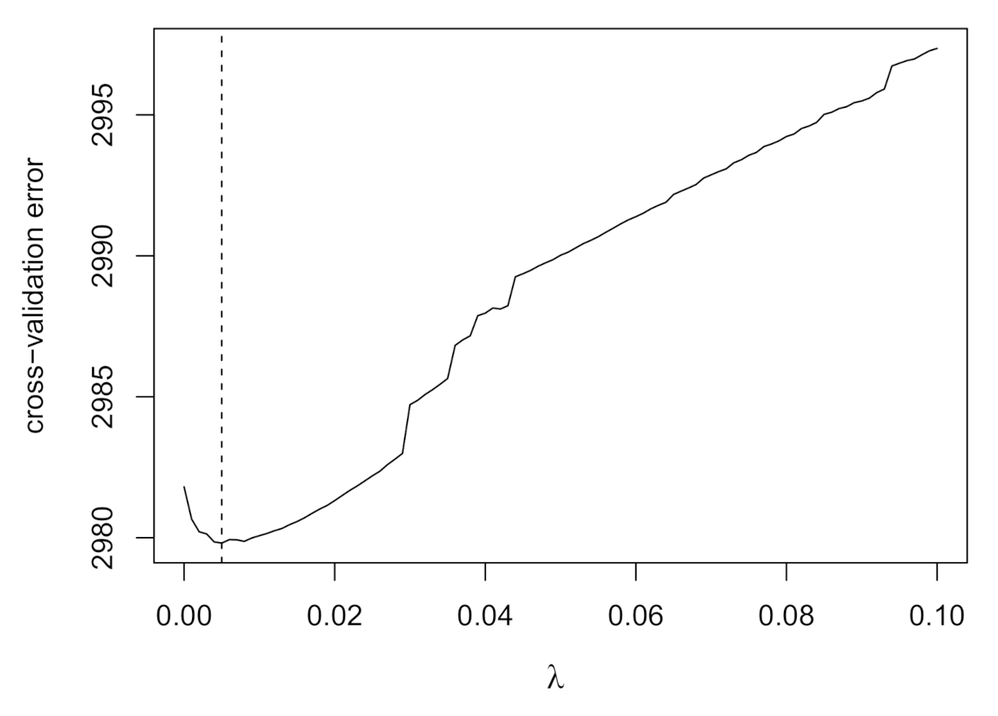
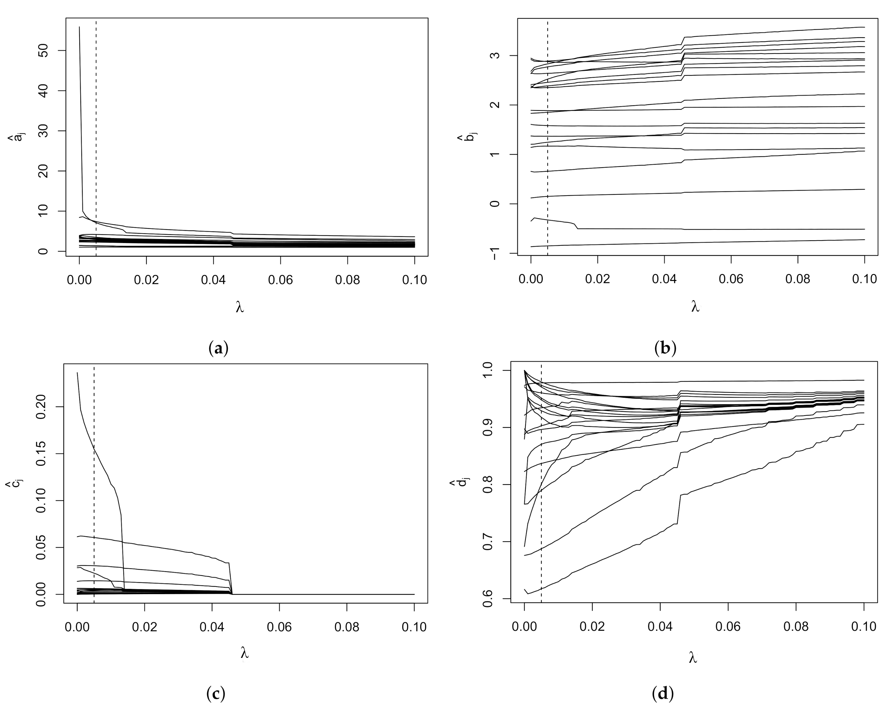
Figure 1 shows the cross-validation error as a function of $\lambda$. The vertical dashed line corresponds to the minimum value, which is for $\lambda =0.005$. Figure 2 shows the item parameter estimates at different values of $\lambda$. The MLE estimates and the penalized estimates at the selected value of $\lambda$ are reported in

Table 5. Item parameter estimates of the ISRD-2 study.

	MLE				Penalized
	${\widehat{\mathit{a}}}_{\mathit{j}}$	${\widehat{\mathit{b}}}_{\mathit{j}}$	${\widehat{\mathit{c}}}_{\mathit{j}}$	${\widehat{\mathit{d}}}_{\mathit{j}}$	${\widehat{\mathit{a}}}_{\mathit{j}}$	${\widehat{\mathit{b}}}_{\mathit{j}}$	${\widehat{\mathit{c}}}_{\mathit{j}}$	${\widehat{\mathit{d}}}_{\mathit{j}}$
BEERLTP	55.90	−0.35	0.24	0.97	7.12	−0.33	0.15	0.98
SPIRLTP	8.42	0.12	0.00	0.82	7.41	0.15	0.00	0.84
HASHLTP	3.94	0.66	0.00	0.62	4.20	0.66	0.00	0.62
XTCLTP	2.71	2.63	0.00	0.77	2.54	2.77	0.00	0.87
LHCLTP	2.31	2.92	0.00	1.00	2.32	2.89	0.00	0.92
VANDLTP	3.08	1.37	0.03	0.97	3.10	1.37	0.03	0.96
SHOPLTP	1.44	1.14	0.03	0.92	1.38	1.17	0.02	0.93
BURGLTP	3.50	2.41	0.00	1.00	3.17	2.46	0.00	0.97
BICTLTP	2.76	1.89	0.00	1.00	2.74	1.89	0.00	0.98
CARTLTP	3.71	2.68	0.00	0.88	3.10	2.83	0.00	0.94
DOWNLTP	1.47	−0.87	0.00	0.89	1.32	−0.85	0.00	0.90
HACKLTP	1.02	2.95	0.00	1.00	1.04	2.88	0.01	0.95
CARBLTP	2.70	2.38	0.00	1.00	2.71	2.35	0.00	0.93
SNATLTP	2.32	2.64	0.01	1.00	2.27	2.64	0.01	0.95
WEAPLTP	2.50	1.61	0.01	1.00	2.57	1.58	0.01	0.97
EXTOLTP	3.54	2.35	0.00	0.69	2.94	2.52	0.00	0.80
GFIGLTP	3.82	1.20	0.06	0.77	3.49	1.25	0.06	0.79
ASLTLTP	2.64	2.35	0.01	0.90	2.54	2.39	0.01	0.90
DRUDLTP	3.33	1.83	0.00	0.68	3.27	1.85	0.00	0.69

. The parameter estimates were obtained using the reg4PL package available as supplementary material to this paper. Since in this example the sample size is rather large, the value of $\lambda$ determined by cross-validation is small. Nonetheless, some resultant parameter estimates are noticeably reduced, such as the discrimination parameters of item BEERLTP, which was extremely high using MLE. As already observed in self-reported delinquency studies [10,11], the lower asymptotes of the 4PL model are nearly zero, while some items present an upper asymptote lower than one. In this application, only item BEERLTP has a lower asymptote considerably greater than zero, probably due to the fact that this behavior is not completely unusual for teenagers with a low level of delinquency. It is also worth noting that the lower asymptote of item GFIGLTP is slightly greater than zero, likely because one could participate in a fight against their will. Various items have an upper asymptote lower than one, such as for example items HASHLTP and DRUDLTP, showing that some behaviors are not necessarily pursued by teenagers at high levels of delinquency. However, it is worth noting that these items are related to the latent variable, as indicated by the highly positive discrimination parameters.

6. Discussion

In this paper we have proposed a regularization method for the 4PL model based on penalized maximum likelihood estimation. While penalized estimation of the linear regression model always introduces bias to reduce the variability of the estimates, in the case under study in this paper the penalty introduced in many cases does not increase the bias and always reduces the root mean square error. In this respect, it is worth noting that the least square estimator used for linear regression provides unbiased estimates of the coefficients, while MLE of nonlinear models is known to be consistent but biased in finite samples. It is also interesting to observe that the values of bias and mean square error reported in this paper are the average over all the items. Thus, considering a single item, it is possible to observe an increment of the bias.

Our approach shares some similarities with the marginalized maximum a posteriori estimation proposed in [13], where some prior distributions are assumed on the parameters and an EM algorithm is then implemented. The main difference between the two approaches lies in the treatment of the parameters of the prior distributions. While in [13] the parameters of the prior distributions are fixed, in our approach the parameter $\lambda$ is estimated by K-fold cross-validation. In this respect, it is important to have only one parameter to estimate, since cross-validation would become impractical for more parameters. Despite there being only one parameter that determines the amount of shrinkage induced by the penalty term, the parameters are shrunk by varying magnitudes, depending on the log-likelihood function. In like manner, the shrinkage of the coefficients of a regression model is governed by a single tuning parameter, when the usual ridge or lasso penalties are employed. It is important to note that the cross-validation error as a function of $\lambda$, as shown for example in Figure 1, suggests that the estimation of the tuning parameter is fundamental, since different values of $\lambda$ can lead to a cross-validation error larger than the one obtained with MLE. The simulation studies show that our proposal is always able to reduce the RMSE and, in many cases, to lower the bias, hence supporting the usefulness of this approach for the 4PL model.

References

- Reise, S.P.; Revicki, D.A. Handbook of Item Response Theory Modeling: Applications to Typical Performance Assessment; Routledge: New York, NY, USA, 2014. [Google Scholar]
- Van der Linden, W.J. Handbook of Item Response Theory; CRC Press: Boca Raton, FL, USA, 2018. [Google Scholar]
- Barton, M.A.; Lord, F.M. An upper asymptote for the three-parameter logistic item-response model. ETS Res. Rep. Ser. 1981, 1981, 1–8. [Google Scholar] [CrossRef]
- Reise, S.P.; Waller, N.G. How many IRT parameters does it take to model psychopathology items? Psychol. Methods 2003, 8, 164–184. [Google Scholar] [CrossRef] [PubMed]
- Waller, N.G.; Reise, S.P. Measuring psychopathology with non-standard IRT models: Fitting the four-parameter model to the MMPI. In Measuring Psychological Constructs with Model-Based Approaches; Embretson, S., Ed.; American Psychological Association: Washington, DC, USA, 2010; pp. 147–173. [Google Scholar]
- Rulison, K.L.; Loken, E. I’ve Fallen and I Can’t Get Up: Can High-Ability Students Recover From Early Mistakes in CAT? Appl. Psychol. Meas. 2009, 33, 83–101. [Google Scholar] [CrossRef] [PubMed]
- Liao, W.W.; Ho, R.G.; Yen, Y.C.; Cheng, H.C. The four-parameter logistic item response theory model as a robust method of estimating ability despite aberrant responses. Soc. Behav. Pers. 2012, 40, 1679–1694. [Google Scholar] [CrossRef]
- Yen, Y.C.; Ho, R.G.; Laio, W.W.; Chen, L.J.; Kuo, C.C. An empirical evaluation of the slip correction in the four parameter logistic models with computerized adaptive testing. Appl. Psychol. Meas. 2012, 36, 75–87. [Google Scholar] [CrossRef]
- Magis, D. A note on the item information function of the four-parameter logistic model. Appl. Psychol. Meas. 2013, 37, 304–315. [Google Scholar] [CrossRef] [Green Version]
- Loken, E.; Rulison, K.L. Estimation of a four-parameter item response theory model. Br. J. Math. Stat. Psychol. 2010, 63, 509–525. [Google Scholar] [CrossRef]
- Culpepper, S.A. Revisiting the 4-parameter item response model: Bayesian estimation and application. Psychometrika 2016, 81, 1142–1163. [Google Scholar] [CrossRef]
- Waller, N.G.; Feuerstahler, L. Bayesian Modal Estimation of the Four-Parameter Item Response Model in Real, Realistic, and Idealized Data Sets. Multivar. Behav. Res. 2017, 52, 350–370. [Google Scholar] [CrossRef]
- Meng, X.; Xu, G.; Zhang, J.; Tao, J. Marginalized maximum a posteriori estimation for the four-parameter logistic model under a mixture modelling framework. Br. J. Math. Stat. Psychol. 2019. [Google Scholar] [CrossRef]
- Hastie, T.; Tibshirani, R.; Friedman, J. The Elements of Statistical Learning: Data Mining, Inference and Prediction, 2nd ed.; Springer: New York, NY, USA, 2009. [Google Scholar]
- James, G.; Witten, D.; Hastie, T.; Tibshirani, R. An introduction to Statistical Learning; Springer: New York, NY, USA, 2013. [Google Scholar]
- Tutz, G.; Gertheiss, J. Rating scales as predictors—The old question of scale level and some answers. Psychometrika 2014, 79, 357–376. [Google Scholar] [CrossRef] [PubMed]
- Tutz, G.; Gertheiss, J. Regularized regression for categorical data. Stat. Model. 2016, 16, 161–200. [Google Scholar] [CrossRef] [Green Version]
- Houseman, E.A.; Marsit, C.; Karagas, M.; Ryan, L.M. Penalized Item Response Theory Models: Application to Epigenetic Alterations in Bladder Cancer. Biometrics 2007, 63, 1269–1277. [Google Scholar] [CrossRef] [PubMed]
- Tutz, G.; Schauberger, G. A penalty approach to differential item functioning in Rasch models. Psychometrika 2015, 80, 21–43. [Google Scholar] [CrossRef] [Green Version]
- Schauberger, G.; Mair, P. A regularization approach for the detection of differential item functioning in generalized partial credit models. Behav. Res. Methods 2020, 52, 279–294. [Google Scholar] [CrossRef]
- Sun, J.; Chen, Y.; Liu, J.; Ying, Z.; Xin, T. Latent Variable Selection for Multidimensional Item Response Theory Models via L1 Regularization. Psychometrika 2016, 81, 921–939. [Google Scholar] [CrossRef] [PubMed]
- Battauz, M. Regularized Estimation of the Nominal Response Model. Multivar. Behav. Res. 2019, 1–14. [Google Scholar] [CrossRef]
- Magis, D.; Tuerlinckx, F.; Boeck, P.D. Detection of Differential Item Functioning Using the Lasso Approach. J. Educ. Behav. Stat. 2015, 40, 111–135. [Google Scholar] [CrossRef]
- Béguin, A.A.; Glas, C.A. MCMC estimation and some model-fit analysis of multidimensional IRT models. Psychometrika 2001, 66, 541–561. [Google Scholar] [CrossRef]
- Bock, R.D.; Aitkin, M. Marginal maximum likelihood estimation of item parameters: Application of an EM algorithm. Psychometrika 1981, 46, 443–459. [Google Scholar] [CrossRef]
- Tibshirani, R. Regression Shrinkage and Selection via the Lasso. J. Roy. Stat. Soc. B Stat. Methods 1996, 58, 267–288. [Google Scholar] [CrossRef]
- Hastie, T.; Tibshirani, R.; Wainwright, M. Statistical Learning with Sparsity: The Lasso and Generalizations; Chapman and Hall/CRC: Boca Raton, FL, USA, 2015. [Google Scholar]
- Tibshirani, R.; Saunders, M.; Rosset, S.; Zhu, J.; Knight, K. Sparsity and smoothness via the fused lasso. J. Roy. Stat. Soc. B Stat. Methods 2005, 67, 91–108. [Google Scholar] [CrossRef] [Green Version]
- Gertheiss, J.; Tutz, G. Penalized Regression with Ordinal Predictors. Int. Stat. Rev. 2009, 77, 345–365. [Google Scholar] [CrossRef]
- Chalmers, R.P. mirt: A Multidimensional Item Response Theory Package for the R Environment. J. Stat. Softw. 2012, 48, 1–29. [Google Scholar] [CrossRef] [Green Version]
- Van Houwelingen, J.C.; Le Cessie, S. Predictive value of statistical models. Stat. Med. 1990, 9, 1303–1325. [Google Scholar] [CrossRef]
- R Core Team. R: A Language and Environment for Statistical Computing; R Foundation for Statistical Computing: Vienna, Austria, 2018. [Google Scholar]
- Eddelbuettel, D.; François, R. Rcpp: Seamless R and C++ Integration. J. Stat. Softw. 2011, 40. [Google Scholar] [CrossRef] [Green Version]
- Eddelbuettel, D.; Sanderson, C. RcppArmadillo: Accelerating R with high-performance C++ linear algebra. Comput. Stat. Data Anal. 2014, 71, 1054–1063. [Google Scholar] [CrossRef] [Green Version]
- Enzmann, D.H.; Marshall, I.; Killias, M.; Junger-Tas, J.; Steketee, M.; Gruszczynska, B. Second International Self-Reported Delinquency Study, 2005–2007. 2015. [Google Scholar] [CrossRef]
Figure 1.
Cross-validation error in the ISRD-2 study. The selected value of corresponds to the vertical dashed line.
Figure 2.
Regularization paths in the ISRD-2 study for: (a) discrimination parameters, (b) difficulty parameters, (c) lower asymptotes, (d) upper asymptotes. The selected value of corresponds to the vertical dashed line.