Automated Test Assembly for Large-Scale Standardized Assessments: Practical Issues and Possible Solutions

Abstract

In testing situations, automated test assembly (ATA) is used to assemble single or multiple test forms that share the same psychometric characteristics, given a set of specific constraints, by means of specific solvers. However, in complex situations, which are typical of large-scale assessments, ATA models may be infeasible due to the large number of decision variables and constraints involved in the problem. The purpose of this paper is to formalize a standard procedure and two different strategies—namely, additive and subtractive—for overcoming practical ATA concerns with large-scale assessments and to show their effectiveness in two case studies. The MAXIMIN and MINIMAX ATA methods are used to assemble multiple test forms based on item response theory models for binary data. The main results show that the additive strategy is able to identify the specific constraints that make the model infeasible, while the subtractive strategy is a faster but less accurate process, which may not always be optimal. Overall, the procedures are able to produce parallel test forms with similar measurement precision and contents, and they minimize the number of items shared among the test forms. Further research could be done to investigate the properties of the proposed approaches under more complex testing conditions, such as multi-stage testing, and to blend the proposed approaches in order to obtain the solution that satisfies the largest set of constraints.

1. Introduction

Starting from the 1960s, the development of computers and sophisticated item banking systems allowed testing agencies to substitute paper-and-pencil (P&P) assessments with computer-based tests (CBTs). Together with the advent of these innovations, the onerous process of manual selection of items to generate test forms has been upgraded with the introduction of automated test assembly (ATA). Practically, ATA consists of assigning to a software the task of choosing the items from the bank, i.e., the available set of calibrated items. Moreover, it is independent of the mode of administration; thus, it increased the efficiency of both P&P and CBT production. The item selection is performed with the goal of fulfilling a set of restrictions and objectives specified by the user through an ATA model and a compatible programming language. In this way, the psychometric and validity properties of the assessment are improved [1,2]. This approach is used by several institutions for educational evaluation. For example, the Italian National Institute for the Evaluation of the Education and Training System (INVALSI) started to implement ATA to support the Italian standardized CBT assessment projects in 2018 [3]. In addition, the Centraal Instituut voor Toetsontwikkeling (CITO) used ATA for the digital central examinations, for the driving license test, and for the second language test. Furthermore, the Federal Institute for Educational Research, Innovation, and Development of the Austrian School System used ATA for the nationwide educational standard assessment in mathematics in 2012 [4].

ATA plays a crucial role, especially in large-scale assessments, since, when the number of examinees is very large, tests must be administered in multiple sessions and locations. Thus, testing organizations need to produce several test forms to overcome security concerns, such as cheating and leaking of information. Moreover, the tests must have minimal or absent overlap while still following fairness principles, i.e., they must be parallel (equivalent) with respect to their statistical and content-related properties [5,6]. Finally, all the test forms must achieve the highest level of precision in the ability measurement. Those requirements are essential to achieve the features of validity and reliability of a testing instance [2,7,8].

Since both the number of test forms to be assembled and the size of the item bank are often very large, the selection of items must be performed automatically by means of a computer and a specific software [9,10,11,12]. Those programs may use greedy heuristics [13,14] or mixed-integer linear programming (MILP) techniques [2,15,16] to find the optimal combination of items under predefined constraints. In these terms, the optimality of a test is defined by its distance from the maximum test information function (TIF), which is the sum of the item Fisher information (IIF) selected to be in the test. On the other hand, the constraints are related to structural properties of the tests, such as content balancing, test length, overlap, item use, word count, etc.

ATA is also a valuable instrument when more advanced testing strategies are applied. As an example, in the multi-stage testing (MST) framework [16], several test forms (called modules) representing different ability levels or content structures must be assembled prior to their adaptive administration. Moreover, multiple parallel versions are usually needed for each module. In this context, ATA is essential to make these tasks operationally feasible. Other approaches to test administration include computerized adaptive testing (CAT) [17], in which the items are assigned one by one to the respondent depending on the most updated estimate of his/her ability. Despite the gain in the accuracy of ability estimation, fully adaptive approaches, such as CAT, have high operational costs (need of sophisticated systems for item administration, continuous item production, etc.). For these reasons, they are hardly implemented in large-scale assessments, unlike ATA.

However, ATA has proven to be a complicated combinatorial optimization problem, especially if overlap constraints have been specified, and its complexity increases with the number of items in the bank and test forms to generate. In the scientific literature, guidelines specific for ATA problems do not exist, although a detailed and predefined plan of action is pivotal in the process of test development. By adopting a standard protocol, it is possible to increase the efficiency of the decision-making to provide a division of roles among the departments (such as item bank maintainers and experts on psychometrics) and to reduce waste, rework, and excess variance for identical activities. Therefore, the aim of this article is to provide a classification of possible issues that can arise when ATA problems for large-scale assessments must be solved, together with a set of strategies to untangle the complexity of the problems. Those approaches seek to identify the sources of the infeasibilities and take resolutive actions. In particular, we propose two unraveling strategies, named additive and subtractive methods, which differ with respect to the process of adding and/or relaxing the constraints of the model. Although the article focuses on large-scale assessments, the proposed methods can also be considered in more simple cases or even for single-test assembly. This article focuses on the MILP approach, and specifically, the MAXIMIN and MINIMAX paradigms for the assembly of several parallel test forms [2] within the item response theory (IRT) framework limited to unidimensional latent variable and dichotomous responses.

The remainder of this article is organized as follows. First, in Section 2, we introduce the MAXIMIN and MINIMAX ATA models together with the general form of an MILP model applied to ATA instances. Subsequently, in Section 3, we explain the challenge that arises with an ATA of a high number of test forms, and afterwards, in Section 4, we propose two strategies that may unravel these issues. The suggested procedures are tested by the MAXIMIN ATA model on the Trends in International Mathematics and Science Study (TIMSS) 2011/2015 science item bank in Section 5 by imposing a highly constrained ATA problem that should produce several parallel tests that are equivalent with respect to their content and optimal with respect to the precision of measurement. In Section 6, we show another application of our standard protocol by optimizing a MINIMAX ATA model on a simulation based on real data coming from the 2017/2018 standardized assessment program of INVALSI. Finally, in Section 7, the results, limitations, and potential improvements of the present work are discussed.

The software used for the assembly is the Julia [18] package ATA.jl, which implements an internal greedy heuristic and allows one to use any MILP solver interfaced by the package JuMP.jl [19]. For our application, the Cbc solver [20] has been chosen for the MILP optimization because it is a valid open-source alternative. The item banks used for the applications in Section 5 and Section 6 and the Julia code written for optimizing the ATA models are available at https://github.com/giadasp/TIMSS_ATA (Supplementary Materials).

2. ATA Models

In the earliest steps of the test assembly, the desiderata about the test forms must be collected from the experts of each specific field to be assessed. Then, they must be translated into a standardized language used in test assembly problems. The standard form of an ATA model comprises an objective function to be optimized subject to many constraints. The constraints define a possibly feasible set of tests for a given item bank, while the objective function expresses the preferences for the tests in that feasible set. If the specifications have been formulated in a simple, concise, and complete way, it is possible to determine whether they are objectives or constraints. These requirements are crucial for a correct translation of the desiderata in the standard language for test assembly problems. An example of verbal test specifications is described in

Table 1. Example of desiderata.

1.	Average p-value of the test is between 0.40 and 0.60
2.	Number of items on applications is equal to 24
3.	Reliability of the test should be as high as possible
4.	Items 73 and 100 are never in the same test
5.	Measurement precision is as close as possible to a target
6.	Items 33, 45, and 12 must be in the same test

, partially extracted from the book of van der Linden [2]. The lines in the table may represent either objectives or constraints; for example, points 1, 2, 4, and 6 are constraints, while 3 and 5 are objectives.

In educational and psychological measurement, the process of test development is guided by strong methodological test theories: classical test theory [21] and IRT [22]. In the IRT framework, the ability of the examinees is measured by a latent variable [22] by using measurement models, such as the Rasch model, the two-parameter logistic (2PL) model, and the three-parameter logistic (3PL) model. In this article, we focus on the unidimensional 3PL IRT model for dichotomous items (i.e., correct/incorrect), which expresses the probability of endorsing an item as a function of the underlying ability and a set of item parameters representing the item properties through an S-shaped curve called the item characteristic function (ICF). The 3PL model has an ICF expressed by the following formula:

$${\mathcal{P}}_i\left(\theta \right)=c_i+(1-c_i)\frac{exp\left(a_i(\theta -b_i)\right)}{1+exp\left(a_i(\theta -b_i)\right)},$$

(1)

where ${\mathcal{P}}_i\left(\theta \right)$ is the probability of a correct answer to item i for an examinee of ability level $\theta$, and the parameters $a_i$, $b_i$, and $c_i$ represent the discrimination, the difficulty, and the pseudo-guessing parameters of item i, respectively. The test characteristic function (TCF) is the sum of the ${\mathcal{P}}_i\left(\theta \right)$ of all items in the test, and it represents the expected score given an ability point. After the estimation of the item parameters and the assembly of a test, the scoring phase deals with the estimation of the ability scores of the candidates. It is possible to understand how precise the test is in measuring a specific latent ability by using the TIF. The IIFs can be easily derived within the framework of the IRT. For the 3PL model, the IIF of item i at ability $\theta$ is equal to

$${\mathcal{I}}_i\left(\theta \right)=a_i^2\frac{1-{\mathcal{P}}_i\left(\theta \right)}{{\mathcal{P}}_i\left(\theta \right)}{\left[\frac{{\mathcal{P}}_i\left(\theta \right)-c_i}{1-c_i}\right]}^2.$$

(2)

A vast literature about ATA models is available, and it is mainly based on MILP techniques; the manual [2] provides an overview of the topic. MILP methods are special representations of the already mentioned desiderata, which must be formulated through linear inequalities. Formally, given a set of optimization variables $x_{it}\in \{0,1\}$, where $i=1,\dots ,I$ are the indices of the items in the item bank and $t=1,\dots ,T$ are the indices of the test forms to be assembled, a generic MILP model for the assembly of T test forms can be written in the following way:

$$\begin{array}{ccccc}\hfill \mathrm{maximize}& \sum _{i=1}^I{q}_{it}{x}_{it}\hfill & & \hfill & \hfill \left(\mathrm{objective}\mathrm{function}\right)\\ \hfill \mathrm{subject}\mathrm{to}& & & \hfill & \end{array}$$

(3a)

$$\begin{array}{ccccc}\hfill & \sum _{i=1}^I{v}_{itm}{x}_{it}\le b_{tm},\hfill & & \forall m,t\hfill & \hfill \left(\mathrm{constraints}\right)\end{array}$$

(3b)

$$\begin{array}{ccccc}& x_{it}\in \{0,1\},\forall i,t,\hfill & & \hfill & \hfill \left(\mathrm{decision}\mathrm{variables}\right)\end{array}$$

(3c)

where $q_{it}$ are the coefficients for the objective function. On the other hand, $v_{itm}$ are the coefficients and $b_{tm}$ is the lower bound for defining the m-th constraint for test t. An example of constraints is the minimum or maximum word count for each test, where the coefficients $v_{itm}$ take the value of the word count of the item i and they are constant amongst tests. Furthermore, we can consider friend sets or enemy sets where the coefficients, by taking a 0 or 1 value, indicate if an item is inside a set or not, respectively. Other examples of constraints that can be specified for each test are: the test length, the number of items with a certain content feature, item use, and the overlap within each of the other tests.

If the expected measurement precision of a single test ($T=1$) at a predefined $\theta$ point has to be maximized, each $q_{it}$ in (3a) takes the value of the IIF of item i. If more than one test should be assembled ($T>1$), the MAXIMIN principle is implemented and the objective function in (3a) is replaced by:

$$\begin{array}{ccccc}\hfill \mathrm{maximize}y& & & & \hfill \left(\mathrm{objective}\mathrm{function}\right)\\ \hfill \mathrm{subject}\mathrm{to}& & \hfill & \end{array}$$

(4a)

$$\begin{array}{ccccc}& \sum _{i=1}^I{q}_{it}{x}_{it}-y\ge 0,\hfill & & \forall i,t,\hfill & \hfill \left(\mathrm{constraints}\right)\\ \hfill & y\in {\mathbb{R}}^{+}.\hfill & & \hfill & \hfill \left(\mathrm{decision}\mathrm{variables}\right)\\ \hfill \end{array}$$

(4b)

In this way, all the TIFs must be higher or equal to the non-negative real-valued variable y, which is maximized.

Another option is to choose absolute targets for the TIF. The targets are the values that the TIF should assume on a fixed number of ${\theta }_k$ points where $k=1,\dots ,K$ along the $\theta$ scale. These values must be chosen by test specialists who know how much precision is required to estimate the abilities of the students at each ability level. That is the reason why absolute targets are used almost exclusively when tests are assembled to be parallel with respect to a known reference test. Formalizing this requirement in the standard form of test assembly models will produce a multi-objective problem that must be reformulated using the MINIMAX approach explained below.

In particular, with the following addition to the model (3a), the TIFs of the resulting tests approach the chosen targets in a finite set of points, ${\theta }_k$, where $k=1,\dots ,K$ on the $\theta$ scale, which we denote as $T_k$:

$$\begin{array}{ccccc}\hfill \mathrm{maximize}y& & & & \hfill \left(\mathrm{objective}\mathrm{function}\right)\\ \hfill \mathrm{subject}\mathrm{to}& & \hfill & \end{array}$$

(5a)

$$\begin{array}{ccccc}& \sum _{i=1}^I{q}_{ik}{x}_{it}-y\le T_k,\hfill & & \forall i,k\hfill & \hfill \left(\mathrm{constraints}\right)\\ \hfill & \sum _{i=1}^I{q}_{ik}{x}_{it}+y\ge T_k,\hfill & & \forall i,k\hfill & \hfill \left(\mathrm{constraints}\right)\\ \hfill & y\in {\mathbb{R}}^{+}.\hfill & & \hfill & \hfill \left(\mathrm{decision}\mathrm{variables}\right)\\ \hfill \end{array}$$

(5b)

where each $q_{ik}$ is the IIF of item i computed at ${\theta }_k$. The more $\theta$ points are chosen, the more the TIF of the assembled tests will meet the desired shape; usually 3–5 points around the peak are enough to have a good approximation.

In order to find the solution to this class of models, which is the best set of values for $x_{it}$, an MILP solver is needed. An MILP solver is a software that finds the most satisfying solution. In order to find the combination of items that is optimal concerning the ATA problem, the model must be written in a formulation like (4a) and translated into the programming language supported by the chosen MILP solver. Examples of open-source solvers written in C are cbc [20] and lp_Solve [23]. Unfortunately, as stated by several benchmarking studies, of which the collection [24] is an example, commercial MILP solvers outperform their open-source counterparts. Nowadays, the best commercial alternatives on the market are CPLEX [25] or Gurobi [26].

3. Frequent Pragmatic Concerns

In large-scale assessments, fairness and security are principles of primary importance. In order to keep the administration safe and valid, the test forms must fulfill a complex set of desiderata and they must have a high quality of measurement. These requirements increase the chance to enlarge the ATA model by adding several new objective variables and constraints, and/or to encounter an infeasible model. The causes of this kind of issue may be the most varied.

First of all, to address security concerns, we may want the tests to have a limited number of items in common. Since pretesting new items is often very expensive and sometimes impossible, item banks are not always large enough to accomplish the mentioned requirement. Thus, a small overlap between test forms is allowed. Overlap constraints are originally not linear (quadratic), so they need to be linearized in order to be accepted by the solver. The linearization heavily increases the number of objective variables (because of the introduction of auxiliary variables) and the number of constraints, making the model very large and reducing the feasible space considerably.

Another difficulty in ATA is to ensure a high level of fairness of the tests. Since, for security needs, the test forms must not be equal, this goal is achieved by making the test forms parallel. A pair of tests is equivalent if they share the same psychometric features and content distributions. The first equivalence is usually obtained by making the TIFs have the same shape and the second by identifying if the most peculiar and relevant content features of the items are equally spread among the forms. More formally, tests are defined to be weakly parallel if their information functions are identical [5]. Tests are strongly parallel if they have the same test length and if they have exactly the same test characteristic function [6].

Sometimes, and more frequently in international assessments, the population of examinees can be partitioned into heterogeneous groups of equivalent average abilities and reserved items. An example of a partition may be a country or a school curriculum. In this context, the fairness of the test is obtained by assembling non-parallel test forms, each one with a TIF peaked at a different ability point adapted to a subpopulation’s proficiency profile or containing specific dedicated items. The process of selection of the best practice is very delicate and it needs that the item bank is rich enough to satisfy all the requirements. A lack of items for a particular content distribution or proficiency profile is very common, and it is very tricky to understand which kind of items are missing.

A list of detailed situations that may occur when an ATA model is solved is reported in the next subsections. In particular, three main classes of issues are identified. The causes that originated the issues are described afterward together with a related example and possible solutions.

3.1. Model Size Growth

The size of an ATA model is defined by the number of variables whose values make the model feasible and/or optimal and by the number of inequality constraints. A small model is easily solvable, and the optimization software needs little memory and time to find its best solution. On the contrary, if the model is too large, the computer may not have enough memory to handle all the variables. In this case, an error or warning is thrown, or an infinite time to evaluate the problem is needed. In particular, if all the constraints and objective function are linear, only the binary variables $x_{it}$ and real variable y defined in (4a) appear in the model. In this case, the size of the model grows with the number of items in the bank, I, and the number of test forms to assemble, T. Thus, the larger the bank is or the more tests are needed, the larger the model is.

Example 1.

An ATA model that assembles$T=5$tests starting from a bank of$I=100$items and with three linear constraints has size$3IT=1500$.

Frequently, it may happen that some constraints are not linear, like in the case of the maximum overlap requirement. Those constraints are originally quadratic and take the following form:

$$\sum _{i=1,\dots ,I}{x}_{it}{x}_{i{t}^{’}}\le {\mathrm{overlapMAX}}_{t{t}^{’}}\forall t\ne t^{’},$$

(6)

where t and $t^{’}$ are the usual indices that identify the test forms and ${\mathrm{overlapMAX}}_{t{t}^{’}}$ is the maximum allowed number of common items between tests t and $t^{’}$. Overlap constraints can be linearized by adding $I(\genfrac{}{}{0pt}{}{T}{2})$ new variables and $(\genfrac{}{}{0pt}{}{T}{2})(1+2I)$ new constraints. As can be noticed, this modification dramatically increases the size of the model. Thus, overlap constraints should be avoided and the number of common items should be limited by working on the maximum item use constraints. In its mathematical formulation, an item use constraint for a generic item i is expressed as:

$${\mathrm{itemUseMIN}}_i\le \sum _{t=1,\dots ,T}{x}_{it}\le {\mathrm{itemUseMAX}}_i,$$

(7)

where ${\mathrm{itemUseMIN}}_i$ and ${\mathrm{itemUseMAX}}_i$ are the lower and upper bounds for the use of the item i, respectively. This inequality imposes that item i must be contained in at least ${\mathrm{itemUseMIN}}_i$ and at most ${\mathrm{itemUseMAX}}_i$ test forms.

Example 2.

The item bank contains$I=100$items; $T=5$tests must be assembled. The overlap between tests is fixed to a maximum of 10 items. Thus, the model has$IT+I(\genfrac{}{}{0pt}{}{T}{2})=1500$optimization variables. Moreover, $(\genfrac{}{}{0pt}{}{T}{2})(1+2I)=2010$consistency constraints are added to the original model. Without any other constraint, the model has size$2010*1500$. Before considering including these constraints in the model, the item use for all the items is limited to 2. If the obtained solution is acceptable, there is no need to increase the size of the model by adding the overlap constraints.

3.2. Infeasibility

The main issue of ATA models is the infeasibility, i.e., no combination of items that satisfies the entire set of constraints exists. In this case, the solver is not able to return any solution and, on rare occasions (e.g., most recent versions of CPLEX), it indicates which constraint is not fulfilled and if there is any incompatibility. However, most solvers do not give any information about the location and strength of the infeasibility. Thus, other inspection strategies must be evaluated. Moreover, previous studies that inspected the topic of infeasibility in ATA problems, such as [27,28], focus on technicalities and mathematical formalisms related to MILP problems. In contrast, this article is centered on practical aspects and pragmatic solutions.

Infeasibilities may be generated by various causes. First of all, the bank may be deficient in certain types of items. In this case, it would be helpful to identify the lacking class of items and to reconsider replenishing the bank with items of that class; otherwise, the maximum item use for those items may be increased. Furthermore, the imposed content distribution must be compared with the actual item disposal in the bank: the more the structure of the tests reproduces the structure of the item bank, the more the ATA model is likely to be feasible.

Example 3.

Consider that$T=7$tests must be assembled, no overlap between forms is allowed, and 10 multiple-choice items are available in the item bank. Maximum item use is fixed at 1 (an item may be used in no more than one test form) and each test must contain at least two multiple-choice items. As is obvious, the item bank may need to be replenished with multiple-choice items in order to fulfill all the requirements. Otherwise, one can decrease T or increase the maximum item use of specific items.

According to [29], content validity is “the degree to which elements of an assessment instrument are relevant to and representative of the targeted construct for a particular assessment purpose.” This definition focuses on elements or pieces of the psychometric construct and how well they are represented in the test through the distribution or blueprint of the domains. The blueprint organizes the test based on the relevant components of the content domain and describes how each of these components will be represented within the test. To establish a certain domain distribution, content constraints may be fixed. This means, for a generic test t, bounding the number of items of a certain class c by a linear constraint of the type:

$$lb\le \sum _{i=1,\dots ,I}{c}_i{x}_{it}\le ub,$$

(8)

where $c_i$ takes value 1 if item i belongs to the class c, and 0 otherwise. Fixing this constraint, test t must contain between $lb$ and $ub$ items with domain c.

Using (8), it is also possible to limit the number of items with any value of a categorical variable and to define its distribution for each form. Examples of categorical variables are the content or cognitive domain, topic, or item type.

Additionally, constraints can be imposed on numeric item features, such as word count or expected score. Formally, a constraint on a generic test t and on the quantitative variable q takes the form:

$$lb\le \sum _{i=1,\dots ,I}{q}_i{x}_{it}\le ub,$$

(9)

where $q_i$ takes the value of the quantitative variable on item i.

If such content specifications are conflicting with the item availability or with each other, the model is infeasible. Two main kinds of infeasibility can occur in ATA:

• Inconsistency or incompatibility between two or more constraints (also called the irreducible infeasible set of constraints (IIS; [28,30]), i.e., the smallest set of constraints, which together cause infeasibility, but for which any proper subset gives a feasible model.
• Too restrictive lower and/or upper bounds.

In practice, an infeasible ATA model may have more than one issue to be solved so that the overall comprehension of the problem may be difficult. To disentangle the question, at least one constraint in each IIS must be eliminated or have its restrictive bounds relaxed to make the solver find a satisfying solution.

Example 4.

IIS: Items 1, 2, and 3 must all be in test 1, but items 2 and 3 are both in the enemy set “ $es$”, so they cannot be chosen to be in the same test. To make the model feasible, either item 2 or item 3 must be excluded from the enemy set “$es$” or they must be allowed to be in separate tests.

Example 5.

Restrictive bounds: Maximum test length is 10, but each test must have at least six items in geography and five items in history. In this case, a reduction of the lower bound of the constraints on geography items is needed.

3.3. Choosing a Solver

Finally, an issue for the practitioners is the choice of the solver to optimize the ATA model, or more generally, an MILP model. This software may differ in the level of the programming language and in the algorithms it implements. The first may be an obstacle if the programming language is of a low level; because it has very little abstraction, it requires one to engineer the memory management, and the code must be compiled before it is used. Example of solvers that are written in a low-level programming languages, such as C or C++, are Cbc and CPLEX. However, some tools to interface the user with the mentioned solvers are available. For example, the package xxIRT [9] wraps the solver lp_Solve. Unfortunately, the latter is widely recognized to not be the best-performing MILP solver available (see [31]). Regarding the optimization methods, the standards for solving an MILP model are the branch and bound [32] or the branch and cut [33] algorithms, but there are numerous alternatives that use heuristics such as genetic algorithms, simulated annealing, and so forth.

This is the reason for why we developed a package specifically designed for ATA written in Julia. Julia is an open-source, stand-alone, high-level programming language, and it offers a fast numeric computation. Our package is called ATA.jl, and it allows one to build and solve an ATA model by means of a graphic user interface or by writing code. Moreover, the user can choose between any compatible MILP solver (both open-source and commercial), such as Cbc, GLPK, Gurobi, or CPLEX. In addition, the package contains a pure Julia ATA solver that implements the simulated annealing heuristic [34], which is suitable for extremely large-scale problems.

4. Unraveling Strategies

In this section, several strategies to identify the issues of an ATA instance and their sources are provided. Once the test assembler is able to understand where the infeasibilities occur, some techniques are advised to find a feasible solution. The strategies differ in the order in which the constraints are evaluated, added, or removed from the model. The process of addition and elimination of constraints may be analogous to the forward and backward techniques proper for the stepwise selection for statistical models [35].

The first step for analyzing the infeasibility of the model may be making a list of the constraints to include in the final ATA model for test production. A preliminary analysis of each constraint consists of optimizing an ATA instance without an objective function that includes only that single constraint. Those instances that the solver declared infeasible must be obviously relaxed. For example, the lower and upper bounds can be decreased or increased to enlarge or narrow the space of possible values from a categorical or quantitative variable. In extreme cases, if a constraint is not absolutely necessary for the final testing purpose, it can be fully relaxed, i.e., eliminated. If the inspection of the results highlighted some item deficiencies, a more costly strategy may be replenishing the item bank. The latter steps must be repeated until the feasibility of all the single ATA instances is achieved.

Example 6.

Suppose that only one test must be assembled. In the form, there must be at least three and at most four questions about the First World War. An ATA instance including only this set of constraints is run, and the solver reports that the model is infeasible. After noticing that the item bank is lacking items about the topic, the history experts decide to adopt a second scenario that they specified for this desideratum. This new setting requires only two items on the topic, so they reduce the lower bound from 3 to 2. With the updated specification, the model is feasible, and the next phases of the analysis can be undertaken.

Once all the single ATA instances are feasible, a priority order of removal or insertion of the constraints in the list must be set. In particular, the specifications and related constraints must be sorted from the most important to the least relevant. For example, if security is a primary concern and cheating behaviors should be discouraged, maximum overlap and item use would be in the top positions. On the other hand, if content validity is the main interest, the tests would overlap more, but constraints on categorical variables must be set with the highest priority.

Example 7.

A national institute for school system evaluation wants to measure the ability in mathematics of$27,000$fifth grade students using a computer-based test. Primary schools have limited technological equipment; thus, the tests cannot be all administrated in one day. To discourage cheating behaviors and leaking of information, the board decided to assemble 15 questionnaires of length 40 with a bounded number of common items between test forms that is set to 5. For the board, security aspects are of primary importance, so the number of test forms and the maximum overlap are selected to be at the top of the priority sequence. Conversely, the length may be reduced down to 37 because the team of psychometricians estimated that the standard error of measurement is acceptably low with 37 items.

The recognized subject matter experts and the management board are fundamental in the preliminary and prioritization phase. Concerning the psychometric aspects, they may evaluate whether some specifications are important in defining the construct to assess and which test features are essential to have a high quality of measurement. More pragmatically, the board appraises to which extent security is a problem and if technical constraints, such as the number and the locations of the administrations, the presence of examinees with special needs, and budget restrictions, may affect the structure of the tests.

For less important specifications, alternatives must be defined in case the solver struggles to assemble the tests. A quality control stage that includes backup plan development should follow. In this phase, the experts evaluate how to modify the bounds of the constraints in order to meet the desired quality standards and reduce the possibility of adversarial restrictions.

Once the priority order and backup plans have been set, the specifications must be passed to the solver in the proper language, and the software may provide a solution that fulfills all the requirements. More frequently, even if the requirements are well specified, correctly written, and individually feasible, no solution for the model including the entire set of constraints exists (i.e., the model is infeasible). Even worse, the solver may take an unacceptably long time to process and solve the model; this is the case of an ATA instance that is too large.

These limitations led us to define two unraveling strategies to quantify the complexity of the ATA instance, identify disagreements among constraints, implement the right measures to disentangle all the knots, and obtain an acceptable feasible solution.

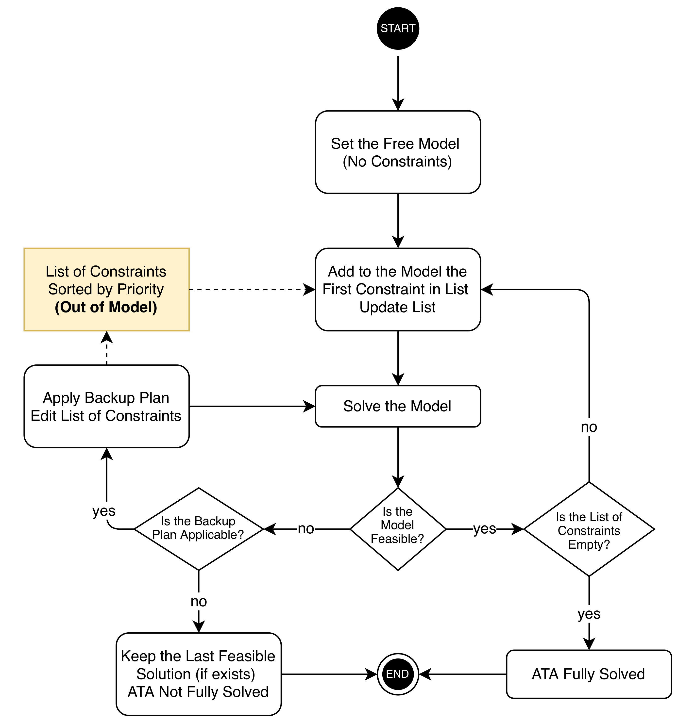
4.1. Additive Method (ADD)

This procedure requires that a group of experts has compiled a list of specifications sorted in descending order of their importance with respect to the goals of the assessment. Then, with no constraints, by the ADD strategy, the assembly starts with the free model, which stores only the optimization variables and the objective function. As the first step, the most important constraint in the list is added, such as the number of test forms and test lengths. If the model is feasible, other constraints, in decreasing order of priority, are included in the model. The process is paused when the model is infeasible. If this happens, the backup plans are implemented; e.g., some constraints are relaxed and the process is restarted from the last feasible model. The assembly task is terminated when (i) the model is infeasible and the constraints cannot be relaxed further (the last step of relaxation is the deletion) or (ii) the model is feasible and all the constraints in the priority order have been added to the model. The ADD algorithm is illustrated in Figure 1.

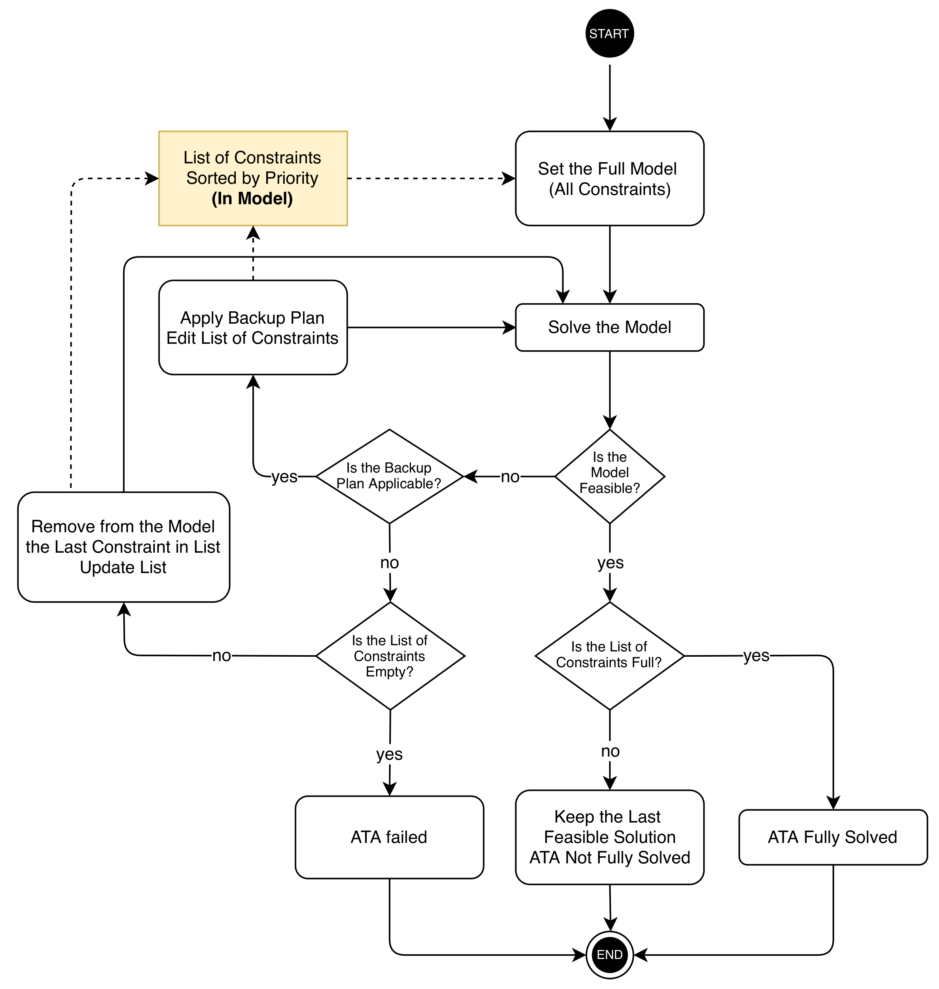
4.2. Subtractive Method (SUB)

The SUB process starts by loading the entire set of constraints in the model in decreasing order of priority. The list of constraints is sorted like in the ADD strategy. The starting model is called full because it loads all the specifications, trying to meet the entire set of requirements. If the model is infeasible, the least relevant constraint, which is in the lowest position of the list, is relaxed, and the model is re-optimized. If, after the relaxation, the list is not empty and the solver cannot find a solution yet, the least relevant constraint is first reconsidered (another backup plan is evaluated if it exists) and then deleted from the list and, hence, from the model. The constraints are sequentially relaxed or eliminated as long as the model is infeasible and the list of constraints is not empty. The procedure is terminated when (i) the model is feasible or (ii) the list of specifications is over. The SUB algorithm is illustrated in Figure 2.

5. Application to TIMSS Data

Institutes that administer large-scale assessments may face the issues described in the previous sections. A real scenario of test assembly is simulated in this article by using the TIMSS survey data. In particular, the data used in this application come from the 2011/2015 TIMSS item bank for the evaluation of the ability of eighth grade students in science. More in general, the TIMSS is a large-scale standardized student assessment conducted by the International Association for the Evaluation of Educational Achievement (IEA). Started in 1995, the project analyzes the skills in mathematics and science of 39 countries every four years, at the end of the final year of secondary school and also in the fourth and eighth grades. Further details regarding this study is available at https://www.iea.nl/studies/iea/timss/2015 (TIMSS 2015 web page). The choice of the subject was driven by the availability of items; in fact, the number of binary response items in science was larger than in mathematics, making the ATA process a meaningful alternative to manual selection. The final bank of items contains 276 dichotomous items, which are listed in Table A1.

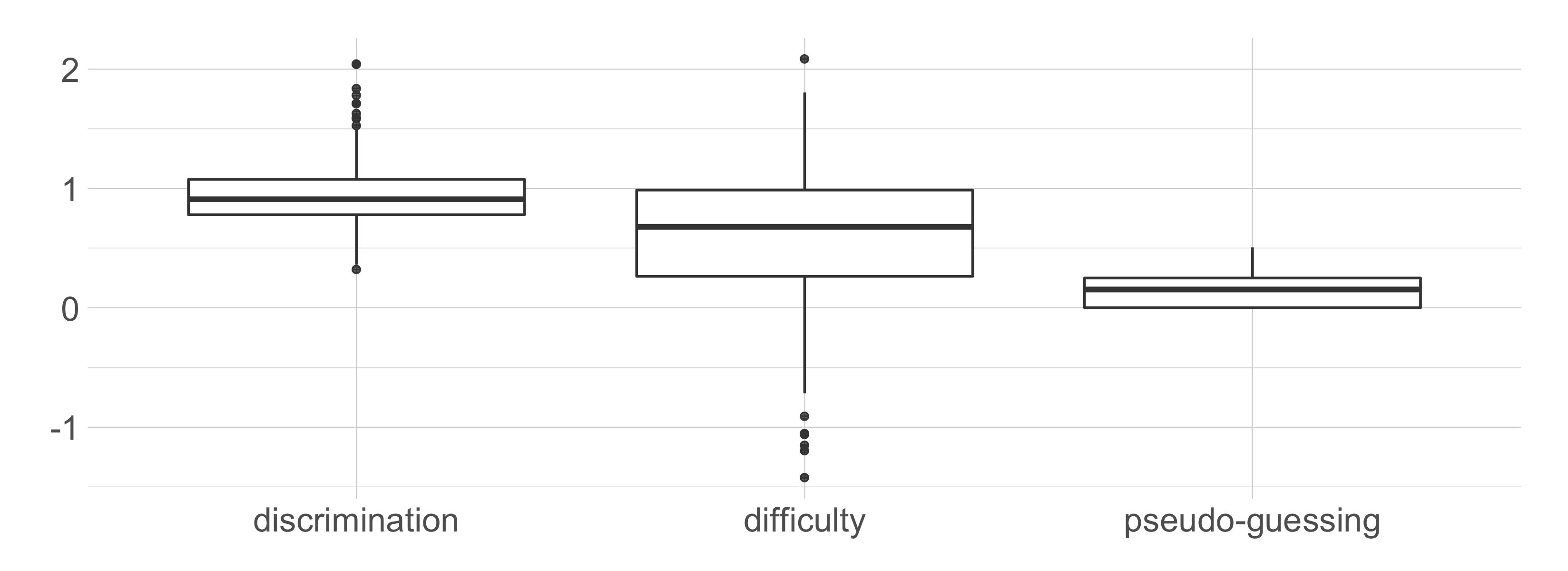
The items are categorized into four content domains (91 biology, 57 chemistry, 54 earth science, 74 physics), three cognitive domains (109 applying, 98 knowing, 69 reasoning), and five topics (108 first topic, 107 second topic, 43 third topic, 16 fourth topic, 2 fifth topic). Furthermore, some items are grouped into 22 units (friend sets). The item bank is calibrated following a 3PL IRT model. Thus, discrimination, difficulty, and pseudo-guessing parameters are available for each item. The discrimination parameter estimates range from 0.321 to 2.043, with a mean of 0.949 and a median of 0.910. On the other hand, the difficulty parameter estimates range from −1.426 to 2.083, with a mean and median equal to 0.598 and 0.680, respectively. Finally, the pseudo-guessing parameters range from zero (125 items have pseudo-guessing parameters equal to zero) to 0.507, with a mean of 0.136 and a median of 0.153. Figure 3 shows the distributions of the item parameter estimates by means of box-plots.

After the item bank has been cleaned and all the variables useful for ATA have been retained, the specifications for the assembly are set following the TIMSS 2015 assessment objectives and indications described in [36] (Chapter 2).

Table 2. List of specifications in decreasing order of priority. TIMSS data.

ID	Priority	Specification	Backup Plan
1	Essential	$T=14$ (Number of test forms)
2	Essential	Test length from 30 to 35
3	High	Maximum item use is 2	Relax upper bound to 3
4	High	From 10 to 13 items in biology
5	High	From 6 to 7 items in chemistry
6	High	From 7 to 9 items in earth science
7	High	From 6 to 7 items in physics
8	Low	For each content domain, at least 2 items for each cognitive domain	Relax lower bound to 1 for items in reasoning
9	Low	Maximum 8 items in common between test forms	Relax upper bound to 10 for adjacent forms

shows the list of constraints in order of priority.

Looking at the list of constraints in Table 2, constraints 1 and 2 are considered essential for satisfying security requirements and for achieving the construct validity of the assessment. In particular, together with the definition of the MAXIMIN objective function, they ensure that several parallel test forms are assembled and that examinees answer a minimum number of questions to obtain the lowest standard error of ability estimate. The zero ability has been chosen as the point the TIFs should be maximized at. In addition, constraints 3 and 9 are useful for overcoming security concerns, since they allow each item to be in no more than two test forms and they limit the number of common items between tests. The latter can be relaxed by allowing the items to be in three different test forms and by increasing the upper bound for the overlap to 10 only for adjacent test forms (e.g., tests 1 and 2, 2 and 3, 3 and 4, etc.), since it is likely that they are administered in the same testing session. Constraints 4–8 are important for content validity. Constraints 4–7 have a high priority because they specify the distribution of the content domains in each test form. On the other hand, constraint 8 has a low priority, as it is a complex and very restrictive requirement, and is unlikely to be fulfilled. In detail, this warrants that the items for each content domain have at least two items in each cognitive domain (e.g., for the six items in physics, two must be in applying, two in reasoning, and two in knowing). This motivated us to prepare a backup plan for constraint 8 in which we ask for only one item in reasoning for each content domain because the bank contains few reasoning items. Thus, the full model contains all the specifications written in the mentioned list. Instead, the empty model just considers the objective function of the MAXIMIN ATA model where the TIF is maximized at an ability equal to 0.

Each constraint was reformulated in linear inequalities and then translated into the language of the ATA interface, which is Julia in our case. The solver used for the lower-level optimization is Cbc. Then, the optimizations were run following the two strategies described in Section 4 using a desktop computer with Windows 10, an AMD Ryzen 3600X processor, and 32 GB of RAM. The latest available version of Julia, i.e., 1.4.1., was used. As a termination criterion, the solver was set to stop when the time of computation reached 500 s. In the next sections, the decision process and the results obtained by the two unraveling strategies are reported.

5.1. Preliminary Analysis of Individual Feasibility

Before the execution of the ADD and SUB strategies, an analysis of each single constraint was conducted by optimizing a separate ATA instance for each requirement in Table 2. This step is crucial to guarantee that each constraint is feasible if taken individually. Constraints on the number of tests, test length, and item use (1, 2, and 3) are considered in all the models, since they are necessary to ensure that test forms have different items. Seven ATA models were optimized, and the included constraints and feasibility are listed in

Table 3. Single automated test assembly (ATA) instances (TIMSS data).

ID	Constraints	Feasible
1	1-2-3	true
2	1-2-3-4	true
3	1-2-3-5	true
4	1-2-3-6	true
5	1-2-3-7	true
6	1-2-3-8	false
6b	1-2-3-8 (backup plan)	true
7	1-2-3-9	false
7b	1-2-3-9 (backup plan)	false

.

Overlap constraints (models 7 and 7b) are not fulfilled even if they are taken individually. In this situation, the solver took the entire time to evaluate the instance, so we do not know if the model is really infeasible or if the solver was not able to find a solution in feasible time because of the model size (44,954 constraints and 25,725 optimization variables). In addition, model 6 is not feasible, but, in this case, the solver produced a solution for its backup plan (model 6b). In the next phases, ADD and SUB strategy are applied to obtain a set of tests that satisfies all the requirements considering the results of the preliminary analysis of feasibility. In particular, constraint 8 is included in the model only in its backup plan, and constraint 9 is fully relaxed.

5.2. ADD Strategy

In the first step, constraints 1 and 2 are added to the free model, and the optimization is performed. The resulting tests have length 35 and, since no item use limit has been imposed, the 35 items with the highest Fisher information functions appear in all the tests. The TIF is equal to 14.159 in zero ability for all the tests. The distributions of the content domain are all equal and are 9, 11, 5, and 10 in biology, chemistry, earth science, and physics, respectively. The distributions of the cognitive domain are 13, 15, and 7 in applying, knowing, and reasoning, respectively. We proceed in step 2 with adding constraint 3 in order to have a realistic scenario where the forms contain different items. The content domain distributions for this and the subsequent steps are illustrated in Table A2. 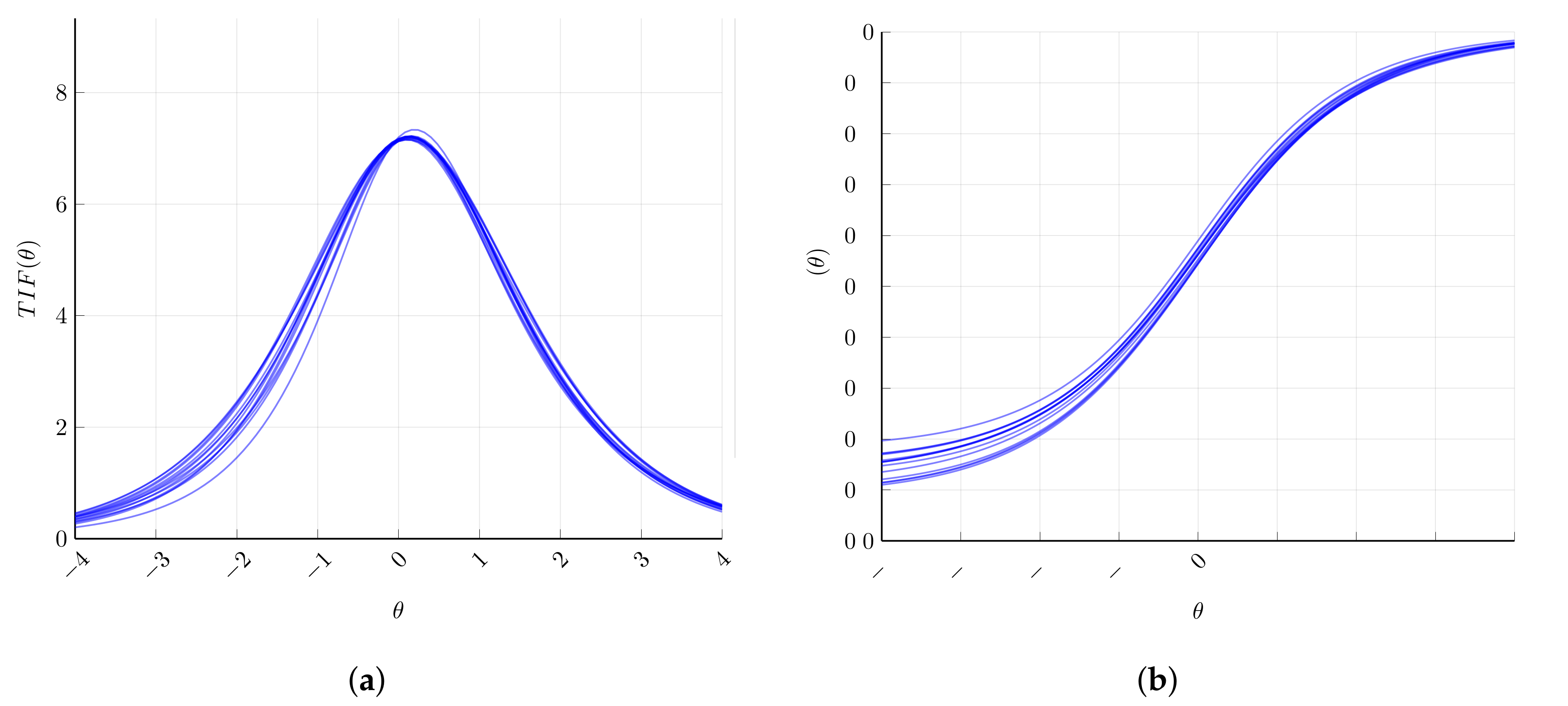Values in red cells do not fulfill the constraints in Table 2. The TIFs at the zero ability point range from 6.971 to 7.046, and the overlap ranges from 0 to 9. Since the model is feasible, constraints 4–7 are added to the model in step 3. The obtained tests have the desired distribution with respect to the content domains, but not all the cognitive domains appear for each value of the content domain. So, in step 4, constraint 8 is applied in its relaxed version. All the requirements have been fulfilled, and constraint 9 is also satisfied without considering it in the ATA model. In particular, the tests have from 0 to 7 items in common. Finally, the resulting TIFs (at ability equal to zero) span from 6.960 to 7.025, as can be seen from Figure 4, where the test characteristic functions (TCFs) rescaled by the test lengths and the TIFs are plotted.

5.3. SUB Strategy

The optimization begins with the full model, which deploys all the specifications except constraint 9 because, as mentioned in Section 3.1 and Section 5.1, it contributes to the model size growth and the open-source solver cannot handle it. Constraint 8 is included in its backup version. The full model is feasible and the results are the same as the ones obtained in step 4 (the last) of the ADD strategy. All the relevant specifications were fulfilled, including the constraints with low priority, even though they were not added to the model.

6. Simulation Based on INVALSI Data

In this application, an item bank was simulated from the data coming from the Italian 2017/2018 INVALSI standardized mathematics assessment. The original P&P INVALSI test was composed of 39 items that were administered to fifth grade students. The items are classified into four domains: 10 items in numbers, 11 items in space and figures, 11 items in data and forecasting, and 7 items in relations and functions. In addition, the distribution of the categorical variable “dimension” is the following: 23 items in knowing, 4 items in arguing, and 12 items in problem solving. Furthermore, some items are grouped into three friend sets: D3, D8, and D12. Before simulating the final item bank, the items were calibrated on the 2017/2018 national sample response data. A unidimensional 2PL model for dichotomous responses was used and the maximum marginal likelihood estimation method [6] was selected. 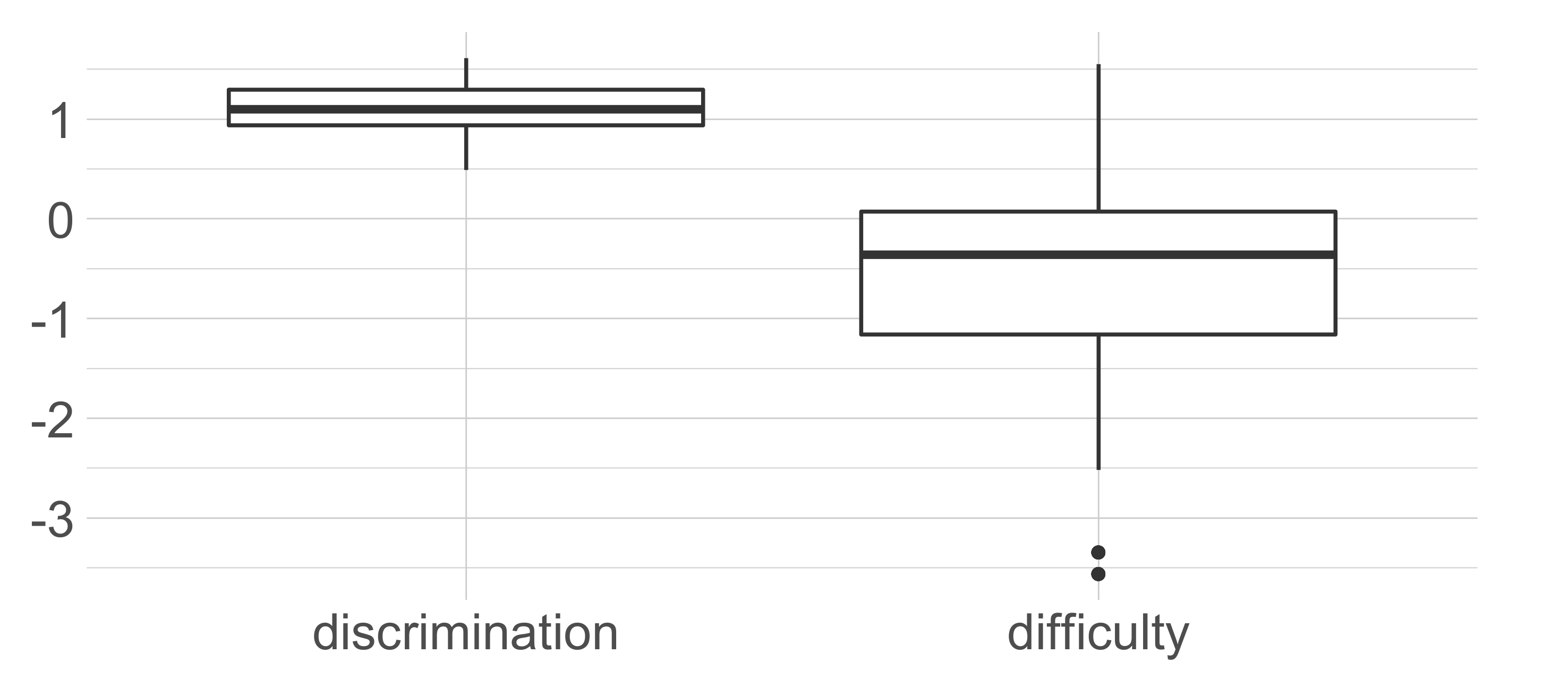Figure 5 shows the resulting distributions of the item parameter estimates.

Unfortunately, the number of administered items was not sufficient to perform a test assembly with a reasonable number of optimization variables. For this reason, we decided to create a simulated item bank of size 300 with approximately the same distributions of domain, dimension, and item parameters as the original test items.

Another categorical variable called “Item type” with the categories of multiple choice, matching, and open ended was simulated. Open-ended items are usually a concern in large-scale assessments because, in most cases, they cannot be automatically corrected. More specifically, they introduce a variable cost, which has a significant impact on the budget, since it depends on how many open-ended items must be corrected by hand. The simulated item bank has the following distribution for the item type: 32 open ended, 50 matching, and 218 multiple choice. Finally, 11 friend sets with two or three items each were simulated.

Subsequently, we started the ATA process by adopting the SUB and ADD strategies in an ATA model with the MINIMAX objective function (5a) and under the specifications summarized in

Table 4. List of specifications in decreasing order of priority (INVALSI data).

ID	Priority	Specification	Backup Plan
1	Essential	$T=20$ (Number of test forms)
2	Essential	Test length from 38 to 40
3	High	Maximum item use is 3
4	High	From 9 to 10 items in numbers	Backup 1
5	High	From 9 to 10 items in space and figures	Backup 1
6	High	From 9 to 10 items in data and forecasting	Backup 1
7	High	From 9 to 10 items in relations and functions	Backup 1
8	Medium	At least 27 multiple-choice items	Backup 2
9	Medium	At least 8 matching items	Backup 2
10	Medium	From 4 to 6 open-ended items	Backup 2
11	Low	From 23 to 26 items in knowing	Fully relax
12	Low	From 9 to 11 items in problem solving	Fully relax
13	Low	From 5 to 8 items in arguing	Fully relax

. We decided to skip the preliminary analysis and go directly to the SUB and ADD strategies in order to show their specific potential for inspecting the problem. Moreover, if the number of constraints is large, optimizing an ATA model for each specification may be costly in terms of time.

A set of $T=20$ tests with lengths from 38 to 40 items was assembled. The already-mentioned friend sets are included in the assembly as constraints. Each item can be used in a maximum of three test forms. Together with the item use requirements, we imposed the tests to have at least nine items and a maximum of 10 items of each of the domains (numbers, space and figures, data and forecasting, and relations and functions). After analyzing the item bank, the backup plan (Backup 1) for constraints 4, 5, 6, and 7 requires one to increase to 4 the maximum use for items in relations and functions, which have the lowest frequency in the bank. The second set of requirements (constraints 8, 9, and 10) was dictated by the limited budget. In particular, we needed to constrain with a medium priority the number of open-ended items and, subsequently, to keep the test parallel, all the other types of items. Again, the backup plan (Backup 2) for this set was chosen after an inspection of the item bank and considering the fact that the number of open-ended items should be bounded. Thus, we allowed the matching items to be present in not more than four forms. The specifications with the lowest priority (constraints 11, 12, and 13) could be fully relaxed if they made the model infeasible.

The overlap among test forms was not constrained, since, as shown in the previous application, it is not handled by the solver because of the large number of auxiliary variables and inequalities that are appended to the model. The TIF must meet the targets $T_k=[10.0,12.0,10.0]$ in ${\theta }_k=[-1.0,-0.5,0.0]$. In this case, the targets and ability points were equal among the tests. The choice of targets and points was dictated by the distribution of item parameters and our interest in measuring the ability of low-proficiency examinees with the highest expected accuracy. The same termination criteria and software as in the previous application were selected.

6.1. ADD Strategy

The process started by including in the model only constraints 1, 2, and 3, which ensure having 20 test forms with lengths from 38 to 40 items and that each item can appear in, at most, three test forms. The model is feasible but, unfortunately, the domain and dimension distributions do not fulfill the imposed specifications. In particular, the domain “relations and functions” has only three items in one test form. This is the first signal that, probably, few items in that domain are available in the bank. We can confirm this assumption when constraint 7 will be added to the model. Constraints 4, 5, and 6 are progressively added; the model is still feasible at step 4 (constraints from 1 to 6), and the domain “relations and functions” now presents more items in each test form, but the domain “data and forecasting” goes over its upper bound of 11 items in five test forms. In step 5, constraint 7 is added and the model is infeasible. The first backup plan is carried out, so the upper bound of item use for “relations and functions” items is increased to four. The alternative works.

In subsequent steps, the first two constraints with medium importance (8, 9) are included in the model. At step 8, constraint 9 makes the model infeasible, so we apply the second backup plan and, again, this repairs the model. All the other constraints (10, 11, 12, and 13) are added to the model and, after 13 steps, the full model is feasible. The entire process took about 5520 s (11 feasible steps of 500 s plus two infeasible steps of about 10 s each). The resulting test forms satisfy all the initial specifications except constraints 7 and 9, which were evaluated in their backup version. In Table A3, the distributions of domains and dimensions of the assembled tests are reported. Each test pair has no more than 11 items in common. The TIFs have the following ranges: $[10.261,10.789]$ at $\theta =-1.0$, $[11.195,11.456]$ at $\theta =-0.5$, and $[10.414,10.838]$ at $\theta =0.0$.

6.2. SUB Strategy

The first model to be optimized is the full model, which deploys the entire list of specifications in Table 4. The full model is infeasible. Progressively, constraints 13, 12, and 11 are relaxed, as they do not have a backup plan, but all the sub-models keep being infeasible. At step 5, the backup plan of constraint 10 is evaluated so the maximum item use of items in “relations and functions” is increased to 4. The ATA sub-models do not have a solution in this step and in the subsequent four steps, where the backup plans of constraints 10, 9, and 8 are evaluated and the related constraints are gradually removed. The model keeps being infeasible until the alternative version of constraint 7 is applied (step 11). Unfortunately, the SUB strategy ends with a model that satisfies only the first seven constraints, and not even entirely, since the first backup plan was used. The content features of final test forms are listed in Table A4. As can be noticed from the red cells that identify the unsatisfied requirements, this strategy does not work well in obtaining the optimal solution to the full model. On the other hand, the feasible model was found after 11 steps and 600 s: 10 steps of about 10 s each, which returned an infeasibility warning, and the last step, which lasted 500 s. The test forms have no more than 11 items in common. Moreover, the TIFs have the following ranges: $[10.389,10.765]$ at $\theta =-1.0$, $[11.233,11.394]$ at $\theta =-0.5$, and $[10.578,10.760]$ at $\theta =0.0$.

7. Discussion

In this article, an extensive list of good practices to be used for ATA problems has been provided with the aim of reducing the inefficiencies that may arise in the process of decision-making. Standardizing the entire procedure with the formalization of the desiderata, the assignment of priorities to the test specifications, the definition of backup plans, and the choice of the solver may help the test assembler to better understand the problems, to find flaws, and to perform the best actions in a short time. In detail, we investigated the positive and negative effects of individually analyzing the constraints or gradually including or removing them in an ATA model by introducing two assembly strategies—namely, additive (ADD) and subtractive (SUB) strategies. The proposed methods were applied to two ATA problems for the construction of several test forms: the first case study employed the 2011–2015 science item bank of the TIMSS large-scale assessment, while the second one relied on a simulated item bank based on the 2017/2018 INVALSI national standardized P&P mathematics test data.

In the first application, the constraints on the distribution of the content domain, cognitive domain, item use, and overlap between test forms were ranked in order of priority of fulfillment. Then, a preliminary analysis on the individual feasibility of the constraints was conducted, and the problematic requirements were relaxed or eliminated. In particular, the constraint on the overlap (9) had to be eliminated and the constraint on the number of items in each cognitive domain for each content domain (8) had to be partially relaxed, since there were few reasoning items in the bank. At the end, the two strategies were implemented and produced the same results.

Using the ADD approach, the decision-maker was able to understand which constraints made the model infeasible when they are added. Fortunately, the model was feasible until the last constraint was added. On the other hand, the SUB method was faster because the final solution, which satisfies all the specifications (with the backup plan of constraint 8), was obtained in the first step, compared to the fourth step of the ADD strategy. In general, the entire procedure generated 14 tests with attractive validity properties. Regarding the construct, the tests have approximately the same estimation precision and the TIFs obtained in the final solution range in a tight interval from 6.960 to 7.025; hence, the standard error of measurement in zero ability is about 0.378. It should be emphasized that the order of priority of the constraints, the definition of backup plans, and the preliminary analysis on the constraints’ feasibility were crucial aspects in this application. They allowed us to find the challenging constraints before running the ADD and SUB strategies and, by adopting the backup plans, it was possible to obtain the desired full model with minimal effort and without making the model too large for the solver, since overlap constraints were not needed. In the end, the analysis of the item bank revealed that the reasoning items were the least numerous, and setting—according to the backup plan of constraint 8—their lower bound to one item was adequate for finding a solution for the ATA problem and a satisfactory set of test forms with a light compromise.

With the aim of adding more evidence of the proposed approaches, a second case study has been presented. In this application, unlike the first one, the item bank was simulated, trying to reproduce the characteristics of a real P&P test administered to Italian pupils. The requirements were sorted in order of priority as well. In this case, the categorical variables under inspection were the content domain, the type, and the dimension of the items. The first variable should have about the same number of items for each category (numbers, space and figures, relations and functions, and data and forecasting), while the item type should satisfy some budget limits regarding the correction of open-ended items. As a requirement of low priority, the dimension could vary across the test forms, but in predefined limited intervals. The preliminary analysis was skipped, and the ADD and SUB strategies were performed immediately in order to show if it was possible to investigate the model issues without individually analyzing the constraints. Instead of preparing relaxations of the bounds as backup plans, the upper limit for the use of items that might have caused issues was increased from 3 to 4.

Using the ADD approach, a problematic constraint was detected in the fifth step, and implementing its backup plan made all the subsequent augmented models feasible until the application of constraint 9. Again, the backup plan solved the issue, making the full model feasible after 13 steps. The gradual addition of the constraints to the ATA model allows one to identify the source of infeasibility by analyzing the last feasible solution. For example, the solution obtained in step 4 was useful for understanding which domain was creating the issue. On the other hand, the SUB strategy was not optimal. The first ten steps were found to be infeasible because of the lack of items in the domain “relations and functions” in the item bank. This result underlines the importance of designing the item bank given the requirements for the tests by means of a blueprint. After relaxing the maximum item use to 4, in the eleventh step, the model was feasible. Unfortunately, the content quality of the test was worse if compared to the tests resulting from the ADD strategy, since constraints 8–13 were not fulfilled in almost every test. A solution could be adopting a hybrid approach between the ADD and the SUB strategies. In other words, after step 10 of the SUB strategy, the ADD strategy could be applied, and constraints 8–13 could be added to the model again. In this way, the same solution of the ADD strategy would be produced, but after 18 steps.

In both the applications, the content validity of the produced tests was preserved, at least for the requirements with the highest priority. Furthermore, the TIFs, and, hence, the precision of measurement of the tests, were sufficiently close to the targets at the specified ability points and ranged in small intervals. Thus, the tests were parallel with respect to both the quality of measurement and the content. In the end, the security concerns were also overcome by building a large number of test forms with a reasonable number of items in common without imposing the problematic overlap constraints.

Overall, the protocols and tools introduced in this work seem to be promising. The two unraveling strategies work adequately and produce appealing results from a practical point of view. However, the study has some limitations that should be improved in the future. First of all, a hybrid approach between the ADD and SUB strategies may be implemented to improve the quality of the results. Moreover, only the case of parallel test assembly was investigated, and the proposed techniques were only tested in two applications. It would be interesting to analyze other cases, such as ATA problems in which the TIFs must be maximized at different ability points or in which the forms contain dedicated items, e.g., a multi-stage testing framework. In addition, the TIMSS item bank holds polytomous items; instead, our application only considers those which are dichotomous. A more realistic scenario would take into account all the items available in the bank. Another challenging application may include assembly under testlet-based and multidimensional IRT models (see, e.g., [37]).