
RALSA: Design and Implementation


1
International Educational Research and Evaluation Institute (Slovenia), SI-1000 Ljubljana, Slovenia
2
Educational Research Institute (Slovenia), SI-1000 Ljubljana, Slovenia
Psych 2021, 3(2), 233-248; https://0-doi-org.brum.beds.ac.uk/10.3390/psych3020018
Submission received: 9 May 2021
/
Revised: 29 May 2021
/
Accepted: 7 June 2021
/
Published: 12 June 2021
(This article belongs to the Special Issue Computational Aspects, Statistical Algorithms and Software in Psychometrics)
Abstract
:International large-scale assessments (ILSAs) provide invaluable information for researchers and policy makers. Analysis of their data, however, requires methods that go beyond the usual analysis techniques assuming simple random sampling. Several software packages that serve this purpose are available. One such is the R Analyzer for Large-Scale Assessments (RALSA), a newly developed R package. The package can work with data from a large number of ILSAs. It was designed for user experience and is suitable for analysts who lack technical expertise and/or familiarity with the R programming language and statistical software. This paper presents the technical aspects of RALSA—the overall design and structure of the package, its internal organization, and the structure of the analysis and data preparation functions. The use of the data.table package for memory efficiency, speed, and embedded computations is explained through examples. The central aspect of the paper is the utilization of code reuse practices to the achieve consistency, efficiency, and safety of the computations performed by the analysis functions of the package. The comprehensive output system to produce multi-sheet MS Excel workbooks is presented and its workflow explained. The paper also explains how the graphical user interface is constructed and how it is linked to the data preparation and analysis functions available in the package.
1. Introduction
The international Large-Scale Assessments and Surveys (ILSAs) are becoming increasingly important for research and policy-making in education. Their methodology, however, is rather complex, and the analysis of ILSAs’ data does not comply with the usual statistical procedures, which assume Simple Random Sampling (SRS). Thus, a specialized software for analyzing ILSAs’ data is needed, taking into account all the statistical complexities (see the next section) that stem from their design. Several such software products exist. The IDB Analyzer [1] is a software providing a user interface that interacts with SPSS [2] and SAS [3] to perform the computations. Few packages for the R programming language and statistical software [4] exist: intsvy [5], BIFIEsurvey [6], and EdSurvey [7]. All of these applications take into account the issues for the analysis related to ILSAs’ design complexities. The number of studies that cover them varies, as does the different types of statistics they can compute.
Recently, a new R package for analyzing ILSAs’ data was released—the R Analyzer for Large-Scale Assessments (RALSA) [8]. The package can work with data from all cycles of a large variety of ILSAs. As of now, RALSA has the following functionality, which will be extended in the future:
- Prepare the data for the analysis:
- ¯
- Convert the SPSS data (or text in the case of the Programme for International Student Assessment (PISA) prior to 2015) files into native R datasets;
- ¯
- Merge the study data files from different countries and/or respondents;
- ¯
- View variable properties (name, class, variable label, response categories/unique values, and user-defined missing values);
- ¯
- Data diagnostic tables (quick weighted or unweighted frequencies and descriptives for data inspection and hypothesis elaboration);
- ¯
- Recode variables.
- Perform analyses:
- ¯
- Percentages of respondents in certain groups and averages on variables of interest;
- ¯
- Percentiles of continuous variables;
- ¯
- Percentages of respondents reaching or surpassing benchmarks of achievement;
- ¯
- Correlations (Pearson or Spearman);
- ¯
- Linear regression, with the option for contrast coding for categorical variables;
- ¯
- Binary logistic regression, with the option for contrast coding for categorical variables.
RALSA brings the following benefits compared to other R packages:
- RALSA brings support for a larger range of large-scale assessments and surveys supported by other available R packages. For example, the R package intsvy can work with data from the Trends in International Mathematics and Science Study (TIMSS), the Progress in International Reading Literacy Study (PIRLS), PISA, the International Computer and Information Literacy Study (ICILS), and the Programme for the International Assessment of Adult Competencies (PIAAC) [5]. RALSA brings support for all cycles of the following ILSAs:
- Civic Education Study (CivED);
- International Civic and Citizenship Education Study (ICCS);
- International Computer and Information Literacy Study (ICILS);
- Reading Literacy Study (RLII);
- Progress in International Reading Literacy Study (PIRLS), including PIRLS Literacy and ePIRLS;
- Trends in International Mathematics and Science Study (TIMSS), including TIMSS Numeracy;
- TIMSS and PIRLS joint study (TiPi);
- TIMSS Advanced;
- Second Information Technology in Education Study (SITES);
- Teacher Education and Development Study in Mathematics (TEDS-M);
- Programme for International Student Assessment (PISA);
- PISA for Development (PISA-D);
- Teaching and Learning International Survey (TALIS);
- TALIS Starting Strong Survey (also known as TALIS 3S);
- RALSA is built for user experience. All functions in the package have a clear and parsimonious syntax. All package functions “recognize” the study design and apply the pertinent statistical algorithms without requiring design specification by the user, unless the user wants it. A unique feature in terms of user experience compared to other R packages for analyzing ILSAs’ data is that it also brings a Graphical User Interface (GUI), which adds convenience for the users, especially the non-technical ones, and those who have limited experience with R. The GUI is written in R as well, and does not rely on any external platform or programming language;
- The package has the capability to convert SPSS data files, as they are provided by the organizations conducting ILSAs, into native R data files. PISA files prior to its 2015 cycle were provided in the ASCII text format along with SPSS import syntaxes. RALSA can convert these into .RData files as well. R has the capability of importing SPSS and SAS files through packages, such as foreign [4], although occasionally, some variables will be imported improperly. The availability of the data in the native R file format provides greater convenience for the analyst. RALSA also imports the user-defined missing values and assigns them properly as user-defined missing codes in the converted datasets. This is quite different from the basic handling of missing values in R, which supports only one missing value type (NA), and from other packages for analyzing ILSAs’ data. For more details, see Section 3.1;
- All other R packages print the outputs as text directly in the R console. This is not convenient for the analyst who has to copy the output and convert it into a tabular output. The only exception is intsvy [5], where the output can be written into a very basic comma-separated values file. Different from other R packages, RALSA brings a comprehensive output system, which exports the results into an MS Excel workbook with multiple sheets grouping different kinds of estimates together by type with cell formatting (for more details, see Section 3.4). This feature is of great help for the analyst, who can use the output tables directly in a publication;
- The IEA IDB Analyzer is very convenient to use and has all of the features listed above. However, it is not open-source and is a proprietary software with a restrictive license. Although it is distributed for free, it actually uses SPSS and SAS to perform the computations, and these come with a very steep price. It also works only under MS Windows. RALSA is open-source and free of charge, and works on any operating system where R can be installed.
All of the features listed above reflect the main advantage RALSA has over other software packages for analyzing ILSAs’ data—a free and open-source tool, built for user experience, which is the main advantage RALSA has over other solutions. RALSA also has an accompanying website [9] with help pages. The help pages provide extensive and detailed step-by-step guides and provide examples for each functionality that RALSA has, along with examples using both the command line or the GUI.
The purpose of this technical article is to present the design of the RALSA package, along with the workflow of its functions with a focus on the following aspects:
- The general internal organization of the package’s functions and their interdependence;
- The common internal structure of the analysis functions and the code they reuse from common objects and functions;
- The use of the data.table package for speed and simplicity of the computations through its capability to compute statistics by group with an internal sub-setting simultaneously;
- The structure and workflow of the output system;
- The GUI design, its structure and the way it is linked to the data preparation and analysis functions.
The article presents illustrative examples with some of the functions of RALSA. It also provides simplified code snippets to demonstrate the basic concepts used in building the package’s functionality.
2. Background
ILSAs possess a complex methodology where data analysis requires methods different from what basic statistics offers. There are two major design issues related to the analysis of ILSAs’ data: sampling and assessment. ILSAs’ purpose is to draw inferences about populations of interest [10]. SRS is traditionally used in social sciences to sample elements from a population. It is, however, not applicable in ILSAs because of a number of operational and statistical complexities. First, exhaustive lists of all students in the target population may not exist to draw an SRS. Second, linking students to their schools and teachers would not be possible. Third, it is not efficient in terms of organizing and conducting a study for populations that can be quite dispersed [11]. This is why ILSAs use multistage stratified cluster sampling where, first, schools are selected with a probability proportional to their size (PPS sampling) within explicit and/or implicit strata, then intact classes with students in the target population are sampled at random within each school. This is the common scenario in studies conducted by the International Association for the Evaluation of Educational Achievement (IEA), such as the Progress in International Reading Literacy Study (PIRLS) (for more details, see [12], for example). PISA, conducted by the Organisation for Economic Co-operation and Development (OECD), takes a slightly different approach where schools are sampled with PPS (with explicit and/or implicit stratification), and the number students in the target population is sampled at random within each school regardless of to which class they belong [13]. This concise description clarifies the main differences between SRS and the sampling strategy used in ILSAs. The main difference is that SRS assumes equal probabilities of selection, while ILSAs use PPS, i.e., unequal probabilities. Another difference is that, with SRS, individual students are sampled from the entire population completely at random, regardless of the school they belong to, while in ILSAs, entire clusters of students within initially selected schools are sampled.
The assessment designs used in ILSAs are complex as well. The usual practice is to collect data on all test items from all students. This can be rather inefficient with complex constructs, especially when the study tests students on multiple constructs. For example, PISA collects data on reading, mathematics, and science literacies [14], which are quite broad content domains. PIRLS’ only construct is reading literacy [15], but this content domain is very broad and versatile. In addition, besides the content domains, these studies also collect data on different cognitive domains. To assess student achievement reliably and validly, a large number of items is required. For example, PIRLS 2016 uses a total of 175 items to estimate reading literacy for different purposes of reading and different comprehension processes [16]. Administering all of the items to all of the students in the sample would take a long time (both physical and psychological) and would result in poor student performance on the items due to student fatigue [17]. Parsimonious, yet efficient, design is needed. Thus, ILSAs use the so-called Multiple Matrix Sampling (MMS) of items where some students take some items. Items are grouped into blocks, and blocks are rotated across a number of booklets where every next booklet has a block in common with the previous booklet, so that a link across booklets is ensured. In the newly developed Computer-Based Assessment (CBA) delivery mode (e.g. in PIRLS), the logic is the same, although not individual items in blocks, but complex tasks are constructed and grouped into task combinations. Every task combination is linked with the next one through a common task [15]. This way, no student takes all items/tasks, and no item/task is delivered to any of the students. This way, a parsimonious and “short” design is ensured.
The parsimony of the sampling and assessment designs described above comes at the expense of increased complexity and the necessity to use analytical methods other than the ones found in statistical textbooks due to the consequences such designs have for the estimation of population parameters and their standard errors. Sampling is not with equal probability, and students are nested in classes (selected clusters) and schools; thus, sampling variance in ILSAs will not be the same as with SRS. Unbiased or consistent estimation of the sampling variance is achieved by using Jackknife Repeated Replication (JRR), as in PIRLS and other studies, or Balanced Repeated Replication (BRR) with Fay’s modification, as in PISA and other assessments and surveys. These are sampling replication techniques where the sampled schools are coupled into sampling zones and each school within a zone is assigned a replication indicator, which determines if a school’s weight shall be increased or decreased. In studies using JRR, respondents in one of the schools in a zone receives the weight doubled, and in the other, the weight is set to zero. In studies using BRR with Fay’s modification, the decision about which school shall have its weight increased or decreased for a given replicate is taken after applying a Hadamard matrix. The weights in this case are not doubled, nor set to zero, but increased or decreased by 50%. Regardless of the resampling technique (JRR or BRR), any population parameter is estimated using each replicate, and the sampling variance is then calculated using special formula [11].
The estimation of the measurement variance is more complex. Given that not all students take all test items, there are many missing data on student performance that are missing by design. The traditional use of Item Response Theory (IRT) can derive test scores with such a design. Although IRT can derive scores through Expected A Posteriori (EAP), Multi-Group Expected A Posteriori (EAP-MG), Maximum Likelihood Estimation (MLE), and Warm’s Weighted Likelihood Estimation (WLE), their variance estimation can be rather biased [18]. Some of these are suitable for individual- and not for group-level proficiency estimation [19], and they are inferior to the scaling methodology used in ILSAs [18,19], which will be outlined rather briefly here. ILSAs use the so-called “plausible values” (PV) methodology where student proficiency is treated as unknown and latent regression population models are used [17]. The achievement items’ IRT parameters are estimated using one-, two- or three-parameter logistic models (1PL, 2PL, and 3PL) for multiple-choice items and a partial-credit model for the open-ended items. The item parameters are then used together with the components extracted by Principal Component Analysis (PCA) from the background data. Only components that account for 90% or more of the variance are used in a process called “conditioning” to obtain the ability distribution. This way, a number of groups is formed based on the student characteristics. The final scores are derived by making five (as in PIRLS) or ten (as in PISA) random draws in the distribution of the group to which each student belongs, that is, each student receives not just one, but several scores. This is because the responses missing by design are imputed in the process, and hence, the measurement variance in ILSAs is often referred to as “imputation variance”. For an overview of the PV methodology, see [17,18,19], and for the actual implementation in PIRLS and PISA, for example, see [20,21]. As a result, when using PVs in an analysis, any statistic has to be estimated with each PV and then averaged.
The computation of the standard error of an estimate is computed taking the sampling and measurement variance. When an estimate does not involve PVs, the standard error equals the sampling variance. When PVs are involved, both the sampling and measurement variances are used. The measurement variance is computed for a set of PVs using the full weight and each of its replicates (see [21,22]).
Given all of the above, it is important to note that each study has its own implementation of the sampling and assessment methodologies and variance estimation techniques. For example, although both PIRLS and the International Civic and Citizenship Education Study (ICCS) use JRR for estimating the sampling error, they differ in the actual implementation. PIRLS uses “full” JRR, where each zone is jackknifed twice, each school in a zone is first added with a double weight, and then, the weight is set to zero, resulting in 150 replicated weights [22]. ICCS, on the other hand, uses “half” JRR, where one school receives a double weight, and the weight of the other one is set to zero, without switching once more, resulting in 75 replicated weights [23]. Many other differences exist across the studies in their computational routines, which is beyond the scope of this paper. For more details, see the technical documentation of the corresponding study.
3. RALSA Internals
3.1. General Internal Organization of Functions in RALSA
Functions in the RALSA package are organized in files—one file per function. Each file contains one function definition. However, a function’s file does not contain all the code and data objects used in all the computations a function performs. Some of the core computations a function performs are organized into a file of common functions and auxiliary objects (common.r), and every time a function is executed, it looks for certain objects and functions located in this file. This approach saves much time for development and prevents code repetition, redundancy, and errors. More details on this can be found in the next subsection.
The package, as mentioned earlier, also brings a GUI. The GUI is built entirely using the R shiny [24] package and some other R packages that add extra functionality to its framework. The GUI is linked to the data preparation and analysis functions. When the user interacts with the keyboard and the mouse to select folders, data files, and select and move variables across the fields, the GUI prepares an internal representation of a calling syntax to a function. In every step, internal checks of whether all conditions are satisfied are performed, and decisions are made to display or hide certain elements from the user and display warnings. As a result, from all user settings, a calling syntax is constructed and passed to a function (data preparation or analysis) to perform the computations. Just as the RALSA data preparation and analysis functions use common objects and functions in the “common.r” file, the GUI ui.r (contains the definitions of the interface objects) and the server.r (instructions on how to build the application and render its elements, display, and process data) also contain common objects and functions pertinent to the GUI. These are used to repeat common operations, display objects and messages in the GUI, or even select default values (see Section 3.5).
The first-time use of the package starts with converting the original data provided by the organization into native .RData data files, which will be used further with any other of the package functions. In the case of IEA and most of the OECD studies, the lsa.convert.data function takes the SPSS (files are also provided in SAS file format; RALSA uses the SPSS files) files in a folder, imports them, applies common operations and some transformations, and saves them into .RData files with their original names. In case the data are from PISA cycles prior to 2015, the data files are provided as ASCII text files with SPSS and SAS import syntaxes. RALSA uses the text files and the SPSS syntaxes to read and convert the text files in the native .RData format. The user may decide to convert the data from just a few countries available in the folder instead of the entire database. This can be done using the ISO argument, passing a vector of country ISO codes to it (fourth, fifth, and sixth character in a file name). This is possible only for studies other than PISA where the data for all countries are provided in one large file per respondent type, as opposed to files per country and respondent type, as in other OECD studies and IEA studies.
Before saving the converted data files, the lsa.convert.data function attaches the following attributes to the data:
- Study name (study)—the name of the study (e.g., PIRLS, PISA, ICCS, etc.);
- Study cycle (cycle)—the year when the cycle was conducted (e.g., 2016 for the PIRLS 2016 cycle);
- Respondent type (file.type)—whose respondent type data (e.g., student, teacher, parent, etc.) is in the file.
In addition, it attaches the variable label as an attribute to each variable. The user may decide to keep the user-defined missing codes for each variable; this is the default option (the missing.to.NA argument is FALSE). At the end, the dataset is converted to a data.table object and keyed by the country ID variable (see Section 3.3). The object in the file has the same name as the file name.
Another important data preparation function is lsa.merge.data. It helps the user merge data from different countries and respondent types. In doing so, it will prevent the user from trying to merge file types that are not supposed to be merged. These checks are performed per study. For example, teacher and student data in PIRLS can (and have to be) merged together in order to use teacher data in an analysis, where the teacher characteristics become attributes of the students. In ICCS, on the other hand, there is no link between the sampled students and the sampled teachers; this is an issue related to the sampling design of the study (see [25] for more details), and teacher data can be analyzed on their own. The lsa.merge.data function recognizes the study and stops with a custom error message if the user attempts merging file types that shall not be merged. When the data are merged, the resulting object is written to a file. The object file.type attribute is updated, adding together the respondent types from the different file types being merged. This is very important, as the analysis functions will read and use the information stored in this attribute to make decisions how the computations shall be performed depending on the study’s design.
The functions’ arguments have unified names and follow the same logic; this makes the user become easily acquainted with the functions’ syntax and apply the arguments consistently regardless of which function is in use. Many of the arguments do not have to be specified explicitly. Some of them have a fixed default value; for example, all analysis functions have the include.missing argument with FALSE as its default value. Others have a default value that is not fixed, i.e., it is dynamically defined based on the properties of the data. More on this can be found in the next subsection.
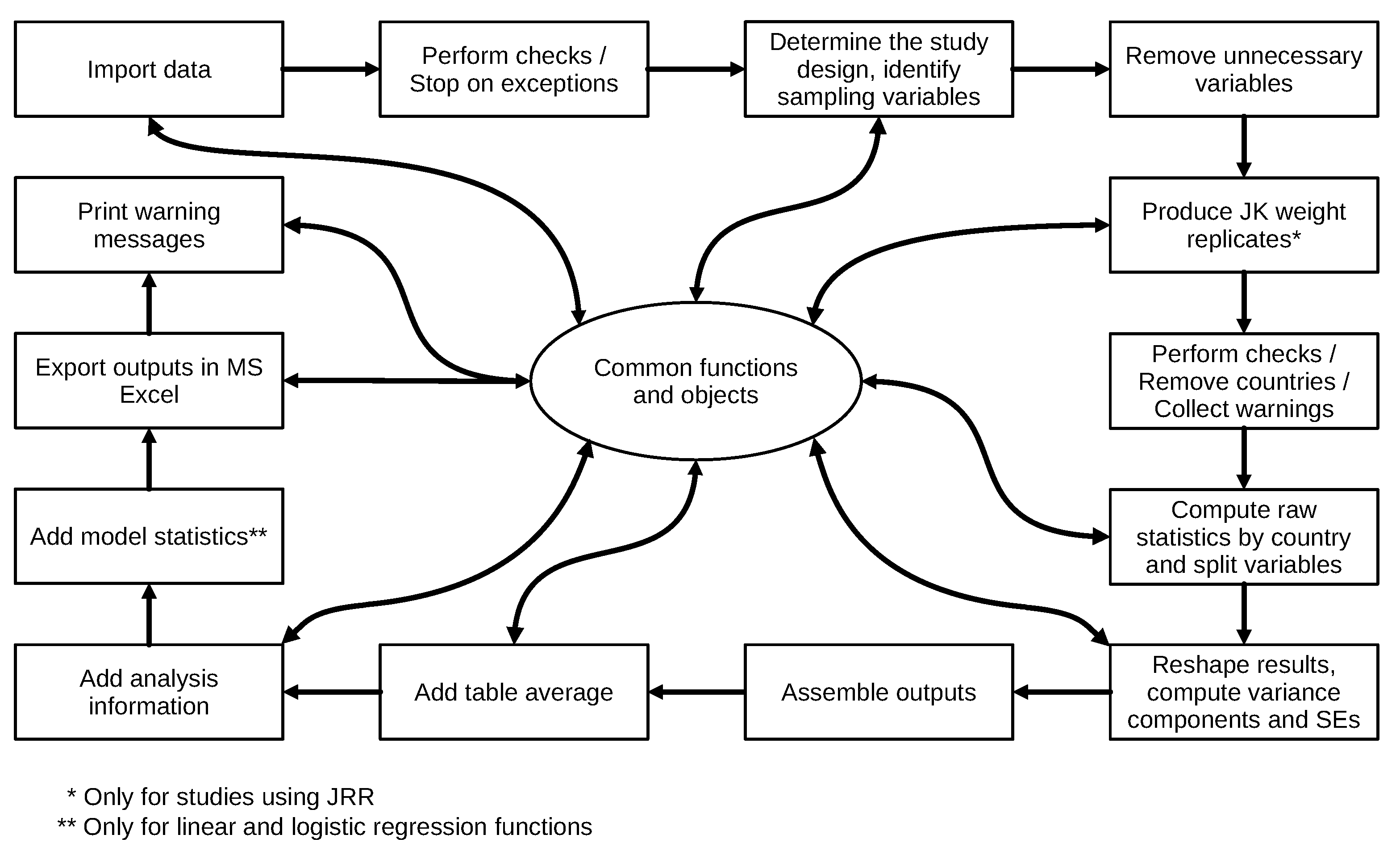
3.2. Structure of the Analysis Functions and Common Code Reuse
The structure and workflow of any analysis function is summarized in Figure 1. As the figure shows, in many steps of the computational process, an analysis function calls functions from the set of common functions and auxiliary objects located in the common.r file. The common functions process the data or perform computations on them and return the results to the analysis function.
For example, when using the lsa.bench function to compute the percentage of students reaching or surpassing a certain performance level, a vector of values for the benchmarks needs to be specified in bench.vals. If left blank, the function will automatically select all benchmark values specified in the study. In PIRLS, for example, these are 400 (Low International Benchmark), 475 (Intermediate International Benchmark), 500 (High International Benchmark), and 625 (Advanced International Benchmark) [26]. However, not all studies have the same benchmarks. ICCS has a different number of performance levels in the different cycles. PISA has different values for the same performance levels in some cycles. Thus, a common object is available in the common.r file (default.benchmarks). If the user does not specify any values for the bench.vals argument (i.e., omits the argument) the lsa.bench function checks the study and cycle attribute of the data (see the previous subsection), matches it against the default.benchmarks object to select the proper benchmark values, and passes them to the bench.vals argument. As mentioned in the previous subsection, this is the dynamic selection of default arguments: if the user does not specify benchmark values, then default values will be determined for the study data in the file or the object in the memory used for the analysis.
Another example of dynamic argument value selection is related to the sampling variables for all analysis functions. The get.analysis.and.design.vars function is called from an analysis function after the data are imported and initial checks are performed. The function checks the attributes (study, cycle, and respondent type; see the previous subsection) of the imported dataset and uses data stored in another common object (design.weight.variables) to determine the correct sampling design variables: default weights, JK zones, and JK replicate indicators (or the available BRR replicated weights in the case of PISA or any other study where BRR design is used). Otherwise, if the user explicitly specifies the weight variable, the analysis function will pass this weight directly, but will still choose the right JK zone and replicate indicator variables (or the BRR replicated weight variables for PISA and other studies with BRR design). Thus, the calling syntax for computing percentages of male and female students and their average overall reading performance can look as simple as in Code Listing 1.
Listing 1:. Example syntax for computing percentages and means.

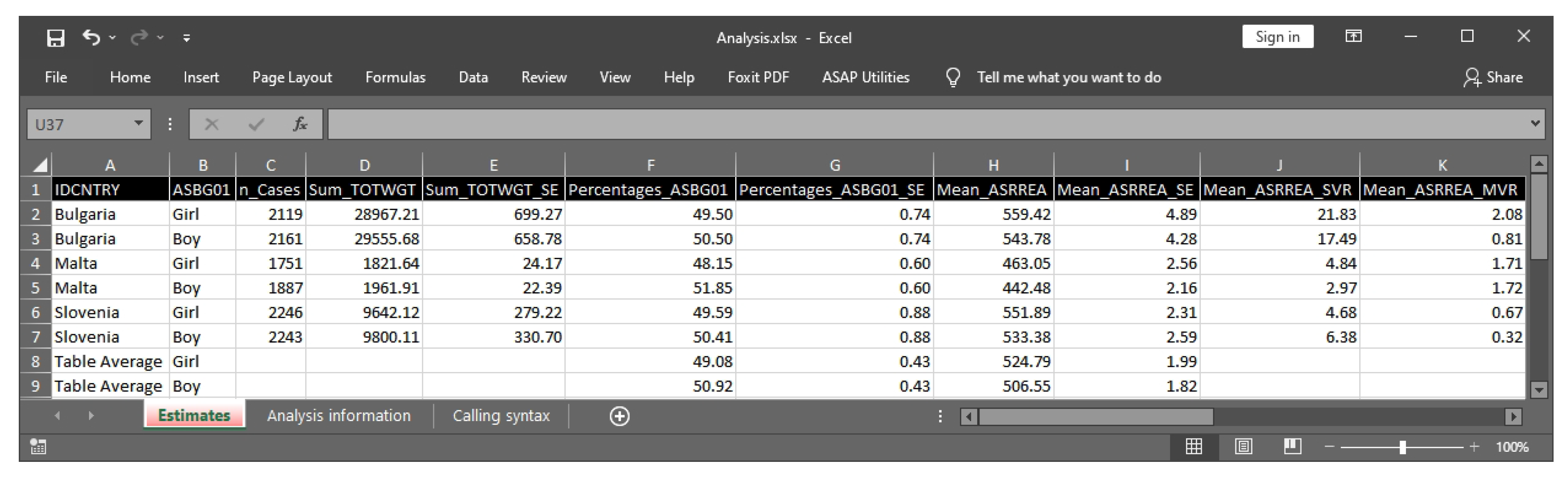
The weight variable is not specified; as described above, it (and all other necessary sampling variables) will be determined automatically. The definition of the PVs for the overall reading achievement takes only the root of their name, ASRREA, and the function will automatically include all PV variables (ASRREA01, ASRREA02, ASRREA03, ASRREA04, and ASRREA05) in the computations. All estimates are computed by country (the country ID variable is added automatically) and student sex (variable ASBG01). If no splitting variables are specified, all statistics will be computed by country only, although the country ID variable is not specified as split.vars. The syntax also does not specify an output file name. In this case, all analysis functions will save an MS Excel file named Analysis.xlsx in the current working directory.
Further, all variables from the imported data that are not relevant for the analysis are removed. This does not only save space in the memory, but also reduces the processing time because the functions (analysis or common) do not have to scroll through all variables initially loaded from the full dataset. If the study uses JRR, the jackknifing replicates are produced. Their number will differ, depending on the design. For example, in ICCS, the number of replicates is 75 with the “half” method, while in PIRLS, the number is 150 with the “full” method, and RALSA will automatically produce them correctly, depending on the study in scope. These two last steps (removing unnecessary variables and producing the replicates) are performed using the produce.analysis.data.table and produce.jk.reps.data functions from the common.r file.
Similarly, when the raw statistics with the full weight in an analysis are computed, a call from the analysis function to a function in the common.r will be made, passing all necessary arguments to it. When the raw statistics are computed, these are passed to another function in common.r to process them further. When using only background variables to compute the means, for example, the raw computed statistics will be passed to the reshape.list.statistics.bckg function. The raw statistics are organized in a list where each component contains the estimates split by country ID, as well as all splitting variables, if provided. The reshape.list.statistics.bckg function from the common.r is called within an analysis function to change the shape of the tables, rename the columns, and compute the sampling and imputation variance and the final standard errors. This common function is called with certain arguments by all analysis functions where statistics involving background variables are computed.
This approach is known as “code reuse” or “software reuse” and is not new: “Software reuse has been practiced since programming began” [27] (p. 529). The purpose of code reuse is to improve software productivity, quality, reliability, and safety [27,28], reduce the development time and, hence, cost [29], and also provide a better maintainability [28]. At the end, even R itself uses this approach through its repository of user-contributed packages using the same idea—written once an R package functionality can be used elsewhere, even in other packages. The implementation of code reuse in RALSA is not just copying and pasting code fragments, but using pre-defined functions that are stored centrally and to which all other functions have access. This reduces code repetition, redundancy, and errors. Any of these common functions is written once and made available elsewhere. If any changes or additions are needed, they are implemented once only without modifying all data preparation and analysis functions.
A relevant question, however, would be why the functions for computing raw statistics, such as linear regression coefficients or means, for example, are located in the common.r file and not nested directly within the analysis function itself (lsa.lin.reg or lsa.pcts.means, respectively) because they are used by these functions only. The locations of any function for computing the raw statistics is in the common.r file for convenience, shorter and clearer analysis functions’ code, and for further developments of the package that may need these. For example, the lsa.prctls function computes percentiles for continuous variables (background or PVs), but the function performing the actual computations is in the common.r file. The lsa.pcts.means computes the arithmetic average of continuous variables. What if the lsa.pcts.means function needs to be extended in the future, so that the user can choose the median as a measure of central tendency instead of the arithmetic average? As we know from basic statistics, the median is the 50th percentile, and wgt.prctl, written to estimate weighted percentiles and located in the common.r file, can be used to compute the 50th percentile as a shortcut to estimate the median. Otherwise, if the wgt.prctl function is nested directly into the lsa.prctls function, it would have to be copied in the lsa.pcts.means file as well or a new function to be written, which will create redundancy and create room for errors. The development of new functionality within the package in future may use other common functions as well.
3.3. Using the data.table Package
RALSA relies heavily on the data.table package [30], not only for processing the data, but also for computing the statistics, which is a distinctive feature of the package. The data.table class inherits from the data.frame class and extends it. The data.table object is very memory efficient and offers speed and easy-to-use syntax to subset data and select and compute on columns by group [31]. The memory efficiency and speed are provided by the internal mechanisms for modification by reference through shallow copies instead of making a copy of the object, modifying it, and, then, overwriting the original object as data.frame would do. Instead, data.table modifies the object by reference, in place [32]. The general data.table syntax for the data.table package is [31] presented in Listing 2.
Listing 2:. General syntax for the data.table package.

where:
- DT is a data.table object;
- i subsets rows using certain criteria;
- j calculates on columns;
- by groups the results by unique values of variables passed to the argument.
Note that there are many other optional arguments than the ones presented in Listing 2, which are just the basic ones. As mentioned above, statistics can be computed directly through the data table syntax. This can be done by group and even while subsetting the data. Let’s say we have merged PIRLS 2016 [33] student data for Bulgaria, Malta, and Slovenia in an object named merged_PIRLS_2016 and we want to compute the number of female and male students in the sample, but only for Bulgaria and Slovenia, not Malta. We can achieve this using the syntax in Code Listing 3.
Listing 3:. Example syntax for computing statistics with the data.table package.

Note how parsimonious the syntax is. We excluded rows for Malta in variable IDCNTRY in i and computed the number of cases in j using the special symbol .N, a built-in variable that holds the number of observations in a group [31], and the groups were defined by the unique values of IDCNTRY (country ID) and ITSEX (student sex). Listing 4 presents the results printed to the R console.
Listing 4:. Example output for computing statistics with the data.table package.

This is a very simple example for a very powerful feature of the data.table package. The same approach, although with a different implementation, was used for all analysis functions. The syntax for another example that computes the weighted arithmetic mean for two continuous variables (“Student Confidence in Reading” and “Students Like reading” scales) by student sex, this time excluding Bulgaria instead of Malta, is presented in Code Listing 5.
Listing 5:. Example syntax for computing statistics with the data.table package.

The syntax subsets the cases, taking out the cases for Bulgaria in IDCNTRY. Further, it loops over columns ASBGSCR and ASBGSLR (the two scales) through lapply and computes the weighted means (using the total student weight—TOTWGT) for each one of them. Note the .SD special symbol: it instructs data.table to take a Subset of Data. It is related to the .SDcols argument, which specifies which columns to be subsetted [31], so all statistics are computed just for these two scales, ASBGSCR and ASBGSLR. The weighted.mean function is used to compute the statistics using the total student weight (TOTWGT). The result is presented in Listing 6.
Listing 6:. Example output for computing statistics with the data.table package.

The above example is an oversimplification of the actual function in RALSA to compute the weighted average for variables using the full weight and all of its replicates in one single run. The examples above demonstrate the utility of the data.table. It is heavily used in RALSA for its speed and memory efficiency. The latter is especially important because of the large sizes of the data files where multiple countries and respondent types may be merged. The concise and simple syntax is an additional advantage. This subsection presented only some of the features RALSA uses from the data.table package. A full presentation of the data.table features goes beyond the purposes of this article. Many other examples demonstrating the power of the package can be found in the data.table vignettes available for it and numerous tutorials available on the Internet.
3.4. Structure and Workflow of the Output System
Traditionally, R prints the results to the console. This is not very convenient for the analyst who needs a tabular output that can be easily modified and laid out in a publication. RALSA has a comprehensive output system to export the final results to an MS Excel workbook with multiple sheets containing estimates and other information related to the analysis. The export.results function is located in the common.r file (for an overview of the common objects and functions, see Section 3.2). The function is called by all analysis functions. Regardless of what the analysis type is, the function exports the results, adding row, column, and cell formatting, and freezes the top row, in a consistent manner. Each output MS Excel workbook has two or more sheets. The first one always contains the results. Another sheet contains the information about the analysis—which data file or memory data object was used, which countries were in the data, which is the study, which weight variable is applied, how many replicated weights, etc. In addition, the workbook also contains a sheet with the calling syntax for the analysis. It can be used to reproduce the analysis if the data changes, e.g., updated datasets or variables were recoded. In the case of linear and logistic regression, the function also adds a sheet with model statistics.
To achieve all this, RALSA relies on the openxlsx package [34]. The package provides many functions to shape, format, add content, and write them to MS Excel files. The function is called within an analysis function after all statistics are computed and starts with identifying which types of outputs (estimates, model statistics, and analysis information are available in the calling environment of the analysis function). It creates a workbook object and adds a sheet for each type of output. Then, it identifies the different types of columns (e.g., percentages, means, correlation coefficients, standard errors, p-values, etc.) for each sheet and applies formatting to rows and columns—background color, font color, number/text type, decimal points, and column widths. The function then writes all the relevant data objects to the sheets and, finally, exports the results to a file on the disk. By default, the MS workbook is opened in the default spreadsheet program immediately after it is exported. If RALSA is used in command line mode, the user may omit specifying the file name for the output. In this case, the analysis function will write the MS Excel file under the generic name “Analysis.xlsx” in the current R working directory. If RALSA is used via the GUI (see the next subsection), the analyst must specify a file name.
A partial screenshot of the output from the percentages and means analysis using the code from Listing 1 is presented in Figure 2.
The MS Excel output from above can be used to produce a graph. Future versions of RALSA will also include the automatic production of graphs, which will be embedded into the MS Excel output files.
3.5. Constructing and Linking the GUI with the Functions
Traditionally, R is used in command line mode. Several R packages are available to provide a means for constructing the GUI using different frameworks. RALSA uses the shiny package [24]. shiny is a web application framework for R, a wrapper for different web technologies that makes creating statistical web applications easy. RALSA uses some other additional R packages that work with shiny to add more functionality to the GUI. This subsection provides an overview of how the GUI is constructed and operates. The main components are presented and explained here.
shiny is intended for developing statistical applications for the web. Statistical applications created with shiny can be executed on a local computer as well, and RALSA uses this feature to provide a GUI in the browser. Each shiny application has two parts. The user interface object definitions and structure of the web applications are stored in ui.r file. The instructions on how to build the application, render its components, process data, and display results are stored in a server logic file server.r. shiny is well known for its utilization of the reactive programming paradigm. It achieves this through the use of reactive values (i.e., data) and reactive events. It also uses observers to observe events and update reactive values or rendered element in the application. Events can be user input or a change in reactive values based on certain conditions [35]. The RALSA GUI uses these techniques to process the imported data and define new reactive objects, which store the user input actions. This provides a very flexible approach towards defining a system call containing the syntax to be passed from the GUI to the data preparation and analysis functions. These occasions will be mentioned further in this subsection.
Usually, a shiny application has statistics computation functions (and even data) added to the server part. RALSA does not add the analysis and data preparation to the web application, but uses them directly once the package is loaded in R, looking directly in the package search path and namespace. There are, however, some common objects and functions that are relevant for the application internal flow control, defining default values, performing checks, and dynamically displaying messages. These objects and functions are similar to the ones in common.r, but relevant to the GUI only. For example, when the user loads a data file in the GUI, the GUI uses common functions to check the name and cycle of the study, as well as the respondent type stored as attributes of the dataset (see the explanations on these in Section 3.1). The GUI will then use these to render them on the screen once the data are loaded, so the user is informed which study, cycle, and respondent types the file contains. Another example is how the PVs are displayed in the tables of available variables and tables with user selection for different fields pertinent to a specific analysis type. The GUI uses a common object with the list of all PVs available in all studies. When the data are loaded, collapse.loaded.file.PV.names reads the all.available.PVs object containing the roots of the PVs (e.g., overall reading achievement PVs are ASRREA01, ASRREA02, ASRREA03, ASRREA04, and ASRREA05, and their root is ASRREA). The function will then modify the list of variables and their labels, replacing an entire set of PVs with its root name, and a variable label will be attached to it, showing how many PVs are related to this PV root name. The PV names and their labels will be removed from the list of variables.
The GUI handles errors and exceptions. For example, if the user tries to add a background variable in a panel that is designated for PV root names only, the GUI will display a warning message and will hide all further elements from the GUI such as the buttons for defining the output file name and executing the syntax to prevent the user from making a mistake. Similarly, if the user decides to add more than one weighting variable, the GUI will automatically remove the additional weighting variable(s), leaving only one in the panel, and will pop up a warning message. This is achieved through reactive values and observers, which handle such unwanted behavior on the user side. However, the major use of reactive values and observers is to control the flow of the entire tab in an application. For example, when the user opens the “Percentiles” analysis tab for the first time after loading the interface in the browser, the tab displays only the button to choose the data file. After a data file is loaded, the panel with available variables, the panels for choosing different types of variables (splitting, background continuous, PVs, and weights), and the selection buttons will be displayed. No other elements—input field for the percentile values, shortcut method check box, and button for defining the output file name—will be displayed until the user chooses either background continuous variables or PVs. After the user selects variables to compute percentiles for, the GUI will display the aforementioned elements, but no other until the output file name is defined. If the user removes the selected variables, all of the aforementioned elements, except for selecting variables, will be removed from the GUI. These behaviors are also achieved through reactive values and observers. Depending on the content of the reactive values (blank or not) for the selected variables’ objects, which change upon user selection, an observer notifies the server to hide or show certain elements. This way, the entire flow of setting an analysis (or data preparation) by the user is monitored, and the GUI prevents misspecification of the analysis.
Traditionally, the shiny applications display the results in the user interface as tables and graphs. Any function (data preparation or analysis) RALSA provides, however, writes the outputs in MS Excel workbooks on the local drive. Thus, the RALSA GUI using shiny takes a different approach. When the user makes or changes settings for an analysis (or data processing) function in the GUI, the selections are captured into reactive values, which are updated every time the user modifies the analysis settings in the GUI. For example, the names of the selected splitting variables are stored in the reactive values object. The events of adding variable names to or removing them from the list of splitting variables are observed all the time. Every time the user adds or removes splitting variables to the list, the reactive object containing the variable names is updated. The names of the selected splitting variables are passed to a reactive expression. Reactive expressions in shiny are normal expressions wrapped into reactive context whose result will change over time [24]. The reactive expressions for the syntax compose an expression for calling a data preparation or an analysis function and are updated in real time, following the user actions. Once the user satisfies all conditions to specify an analysis, the GUI will render the syntax in a read-only text field in the GUI, and an “Execute syntax” button will appear in the GUI.
The final step is to pass the composed syntax to R for execution. When the “Execute syntax” button is pressed, the server will trigger an event handler, which will, in turn, parse the reactive expression for evaluation to R. This step also includes rendering console output directly in the GUI. The console in the GUI is a text output field, whose appearance is also triggered by pressing the “Execute syntax” button. The progress messages are printed in the GUI console using the html function from the shinyjs package [36]. When a new line is appended to the output, the GUI console automatically scrolls down. This feature is very helpful for the user, who does not have to switch to R to follow the progress of the operations through the messages printed in the console.
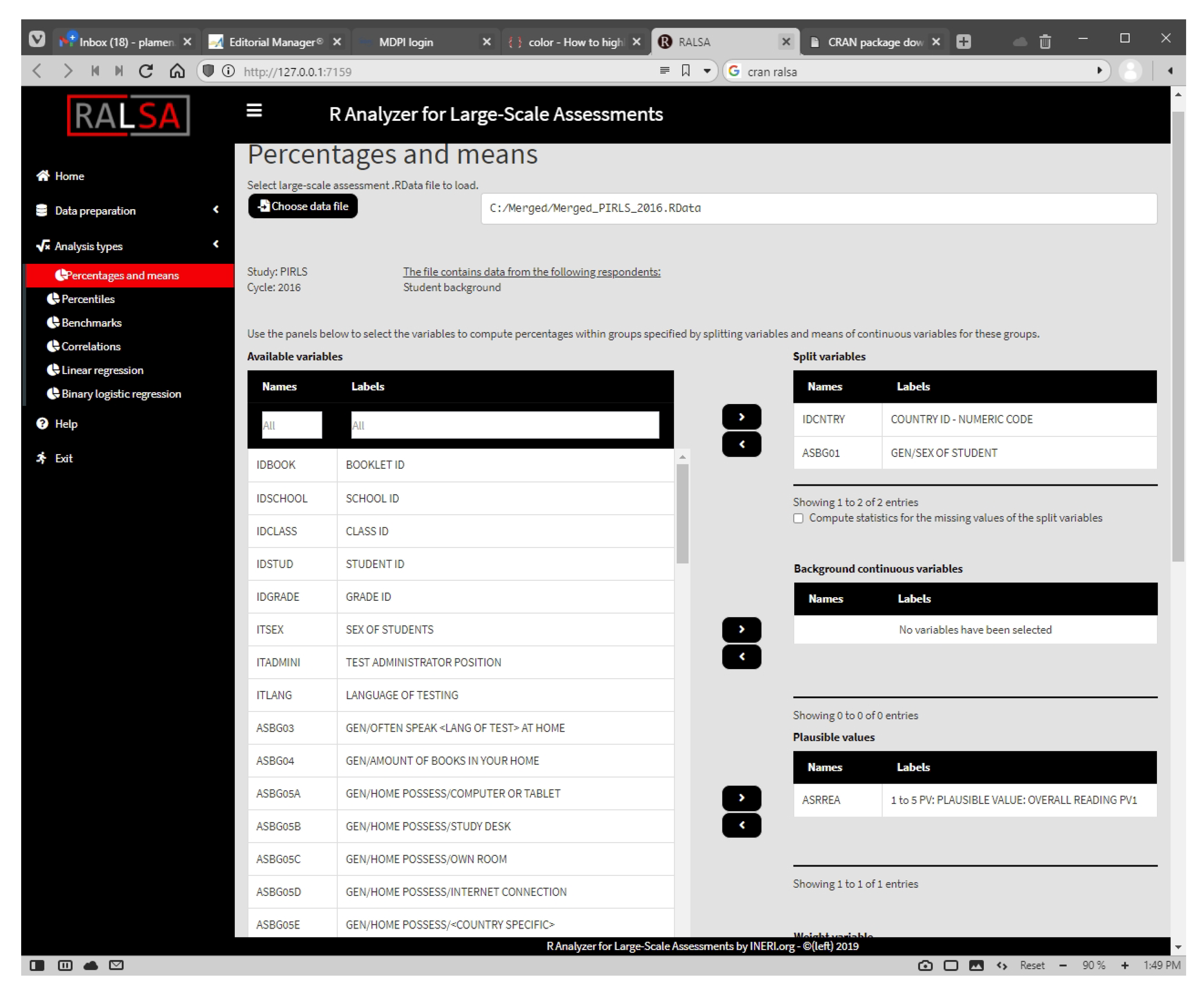
When the package is loaded, a menu is displayed offering the user to start the GUI immediately. Pressing 1 and Enter from the keyboard does so. Alternatively, if the package is already loaded, the user can start the GUI by executing the command in Listing 7. A partial screenshot of the GUI with the settings for the percentages and means analysis equivalent to the code is presented in Figure 3.
Listing 7. Syntax for starting the GUI.

4. Summary and Discussion
A number of software packages for analyzing ILSAs’ data exist. This article presented RALSA, a newly developed R package for analyzing ILSAs’ data. The package can analyze data from various studies using complex sampling and assessment designs. The package was built for user experience and brings a number of features that help even the analysts without technical skills to analyze ILSA data. The package has easy-to-use syntax, automatic recognition of the study design and application of the proper computations, comprehensive output export in an MS Excel workbook, and a GUI for the ease of the analyst.
The article presented the technical aspects of RALSA and its design. The package was designed on the principle of reusing code for common operations, shared across multiple functions to avoid code repetition, redundancy, and errors. The organization and the entire workflow of the package lay on this principle. The analysis and data preparation functions reuse common functions and objects to perform certain operations consistently and safely, regardless of which study’s data are used in an analysis. Besides these benefits, this design also brings one more big advantage—future features can be added to RALSA more consistently, and much faster, compared to the common practice of writing new functionality from scratch. The implementation of generic components may require an investment, which can pay off in the long run through their reuse, which, in turn, enhances the quality of products by using fully tested and debugged software [37]. The advantages of this approach will allow RALSA to grow in the future, adding more studies using complex sampling and assessment designs, as well as more analysis types, by reusing common objects and functions. Suggestions for adding support for new studies (national or international) are welcome. Such was the case of the OECD’s PISA for Development study (PISA-D), which was added after a request from a researcher had been made almost immediately after the first release of the package. Suggestions for adding new analysis types or the addition of features to the existing ones are welcome as well.
The motivation to develop, adapt, and reuse code, however, can go beyond one’s own needs [28], that is, code can be developed and shared with the rest of the software developers for subsequent reuse in other software projects. At the end, “Code reuse is a form of knowledge reuse in software development, which is fundamental to innovation in many fields” [37] (p. 180). This relates to faster and better development of new software in the future. For example, a study from Sojer and Henkel [28] shows that the main benefits Open Source Software (OSS) developers see in code reuse are efficiency and effectiveness. RALSA also uses this approach for faster and safer development by borrowing the functionality from other R packages, as shown earlier in the paper. RALSA is an OSS project as well, just as R and the rest of the contributed packages’ R repository, and is licensed under the General Public License (GPL) v2.0, which permits other developers to reuse its code in their work, after complying with the conditions set in the license agreement.
Funding
This research received no external funding.
Institutional Review Board Statement
Not applicable.
Informed Consent Statement
Not applicable.
Data Availability Statement
Publicly available datasets were analyzed in this study. These data can be found here: https://www.iea.nl/data-tools/repository/pirls (accessed on 10 June 2021).
Acknowledgments
The author of this paper acknowledges the financial support of the International Educational Research and Evaluation Institute (INERI).
Conflicts of Interest
The author declares no conflict of interest.
Abbreviations
The following abbreviations are used in this manuscript:
| 1PL | One-Parameter Logistic model |
| 2PL | Two-Parameter Logistic model |
| 3PL | Three-Parameter Logistic model |
| BRR | Balanced Repeated Replication |
| CBA | Computer-Based Assessment |
| EAP | Expected A Posteriori |
| EAP-MG | Multi-Group Expected A Posteriori |
| GPL | General Public License |
| GUI | Graphical User Interface |
| ICCS | International Civic and Citizenship Education Study |
| IEA | International Association for the Evaluation of Educational Achievement |
| ILSAs | International Large-Scale Assessments and surveys |
| IRT | Item Response Theory |
| JRR | Jackknife Repeated Replication |
| MLE | Maximum Likelihood Estimation |
| MMS | Multiple Matrix Sampling |
| OECD | Organisation for Economic Co-operation and Development |
| OSS | Open-Source Software |
| PCA | Principal Component Analysis |
| PIRLS | Progress in International Reading Literacy Study |
| PISA | Programme for International Student Assessment |
| PPS | Probability Proportional to Size |
| PVs | Plausible values |
| RALSA | R Analyzer for International Large-Scale Assessments |
| SRS | Simple Random Sampling |
| WLE | Warm’s Weighted Likelihood Estimation |
References
- IEA. IDB Analyzer [Computer Software Manual]; (Version 4.0.39). 2021. Available online: https://www.iea.nl/data-tools/tools#section-308 (accessed on 10 June 2021).
- IBM. IBM SPSS [Computer Software]; (Version 27.0). 2020. Available online: https://www.ibm.com/analytics/spss-statistics-software (accessed on 10 June 2021).
- SAS Institute. SAS/STAT Software [Computer Software]; (Version 9.4M7). 2020. Available online: https://www.sas.com/en_us/software/stat.html (accessed on 10 June 2021).
- R Core Team. Foreign: Read Data Stored by ’Minitab’, ’S’, ’SAS’, ’SPSS’, ’Stata’, ’Systat’, ’Weka’, ’dBase’, … [Computer Software Manual]; (R Package Version 0.8-81). 2020. Available online: https://cran.r-project.org/package=foreign (accessed on 10 June 2021).
- Caro, D.; Biecek, P. intsvy: International Assessment Data Manager [Computer Software Manual]; (R Package Version 2.5). 2021. Available online: https://cran.r-project.org/package=intsvy (accessed on 10 June 2021).
- BIFIE; Robitzsch, A.; Oberwimmer, K. BIFIEsurvey: Tools for Survey Statistics in Educational Assessment [Computer Software Manual], (R Package Version 3.3-12). 2019. Available online: https://cran.r-project.org/package=BIFIEsurvey (accessed on 10 June 2021).
- Bailey, P.; Emad, A.; Huo, H.; Lee, M.; Liao, Y.; Lishinski, A.; Nguyen, T.; Xie, Q.; Yu, J.; Zhang, T. EdSurvey: Analysis of NCES Education Survey and Assessment Data [Computer Software Manual]; (R Package Version 2.6.9). 2021. Available online: https://cran.r-project.org/package=EdSurvey (accessed on 10 June 2021).
- Mirazchiyski, P.; INERI. RALSA: R Analyzer for Large-Scale Assessments [Computer Software Manual]; (R package version 1.0.1). 2021. Available online: https://CRAN.R-project.org/package=RALSA (accessed on 10 June 2021).
- INERI. RALSA: R Analyzer for Large-Scale Assessments. 2021. Available online: http://ralsa.ineri.org/ (accessed on 10 June 2021).
- Rutkowski, L.; Gonzalez, E.; von Davier, M.; Zhang, Y. Assessment Design for International Large-Scale Assessments. In Handbook of International Large-Scale Assessments: Background, Technical Issues, and Methods of Data Analysis; Rutkowski, L., von Davier, M., Rutkowski, D., Eds.; CRC Press: Boca Raton, FL, USA, 2014; pp. 74–95. [Google Scholar]
- Rust, K. Sampling, Weighting, and Variance Estimation in International Large-Scale Assessments. In Handbook of International Large-Scale Assessments: Background, Technical Issues, and Methods of Data Analysis; Rutkowski, L., von Davier, M., Rutkowski, D., Eds.; CRC Press: Boca Raton, FL, USA, 2014; pp. 117–154. [Google Scholar]
- LaRoche, S.; Joncas, M.; Foy, P. Sample Design in PIRLS 2016. In Methods and Procedures in PIRLS 2016; Martin, M., Mullis, I., Hooper, M., Eds.; Lynch School of Education, Boston College: Chestnut Hill, MA, USA, 2017; pp. 3.1–3.34. [Google Scholar]
- OECD. Sample Design. In PISA 2015 Technical Report; OECD: Paris, France, 2017; pp. 65–87. [Google Scholar]
- OECD. Test design and test development. In PISA 2015 Technical Report; OECD: Paris, France, 2017; pp. 29–55. [Google Scholar]
- Martin, M.; Mullis, I.; Foy, P. Assessment Design for PIRLS, PIRLS Literacy, and ePIRLS in 2016. In PIRLS 2016 Assessment Framework, 2nd ed.; Mullis, I.V.S., Martin, M., Eds.; Lynch School of Education, Boston College: Chestnut Hill, MA, USA, 2015; pp. 55–69. [Google Scholar]
- Mullis, I.; Prendergast, C. Developing the PIRLS 2016 Achievement Items. In Methods and Procedures in PIRLS 2016; Martin, M., Mullis, I., Hooper, M., Eds.; Lynch School of Education, Boston College: Chestnunt Hill, MA, USA, 2017; pp. 1.1–1.29. [Google Scholar]
- Von Davier, M.; Sinharay, S. Analytics in International Large-Scale Assessments: Item Response Theory and Population Models. In Handbook of International Large-Scale Assessments: Background, Technical Issues, and Methods of Data Analysis; Rutkowski, L., von Davier, M., Rutkowski, D., Eds.; CRC Press: Boca Raton, FL, USA, 2014; pp. 155–174. [Google Scholar]
- Wu, M. The role of plausible values in large-scale surveys. Stud. Educ. Eval. 2005, 31, 114–128. [Google Scholar] [CrossRef]
- Von Davier, M.; Gonzalez, E.; Mislevy, R. What are plausible values and why are they useful? IERI Monogr. Ser. 2009, 2, 9–36. [Google Scholar]
- Foy, P.; Yin, L. Scaling the PIRLS 2016 Achievement Data. In Methods and Procedures in PIRLS 2016; Martin, M., Mullis, I., Hooper, M., Eds.; TIMSS & PIRLS International Study Center: Chestnunt Hill, MA, USA, 2017; pp. 12.1–12.38. [Google Scholar]
- OECD. Scaling PISA data. In PISA 2015 Technical Report; OECD: Paris, France, 2017; pp. 127–186. [Google Scholar]
- Foy, P.; LaRoche, S. Estimating Standard Errors in the PIRLS 2016 Results. In Methods and Procedures in PIRLS 2016; Martin, M., Mullis, I., Hooper, M., Eds.; Lynch School of Education, Boston College: Chestnut Hill, MA, USA, 2017; pp. 4.1–4.22. [Google Scholar]
- Schulz, W. The reporting of ICCS 2016 results. In International Civic and Citizenship Education Study 2016 Technical Report; Schulz, W., Carstens, R., Losito, B., Fraillon, J., Eds.; IEA: Amsterdam, The Netherlands, 2018; pp. 245–256. [Google Scholar]
- Chang, W.; Cheng, J.; Allaire, J.; Xie, Y.; McPherson, J. Shiny: Web Application Framework for R [Computer Software Manual]; (R Package Version 1.6.0). 2021. Available online: https://cran.r-project.org/package=shiny (accessed on 10 June 2021).
- Brese, F. Analyzing the ICCS 2016 data using the IEA IDB Analyzer. In ICCS 2016 User Guide for the International Database; Köhler, H., Weber, S., Brese, F., Schulz, W., Carstens, R., Eds.; IEA: Amsterdam, The Netherlands, 2018; pp. 33–36. [Google Scholar]
- Mullis, I.; Prendergast, C. Using Scale Anchoring to Interpret the PIRLS and ePIRLS 2016 Achievement Scales. In Methods and Procedures in PIRLS 2016; Martin, M., Mullis, I., Hooper, M., Eds.; Lynch School of Education, Boston College: Chestnunt Hill, MA, USA, 2017. [Google Scholar]
- Frakes, W.; Kang, K. Software Reuse Research: Status and Future. IEEE Trans. Softw. Eng. 2005, 31, 529–536. [Google Scholar] [CrossRef]
- Sojer, M.; Henkel, M. Code Reuse in Open Source Software Development: Quantitative Evidence, Drivers, and Impediments. J. Assoc. Inf. Syst. 2010, 11, 868–901. [Google Scholar] [CrossRef] [Green Version]
- Fichman, R.; Kemerer, C. Incentive compatibility and systematic software reuse. J. Syst. Softw. 2001, 57, 45–60. [Google Scholar] [CrossRef]
- Dowle, M.; Srinivasan, A. data.table: Extension of ’data.frame’ [Computer Software Manual]; (R Package Version 1.14.0). 2021. Available online: https://CRAN.R-project.org/package=data.table (accessed on 10 June 2021).
- Introduction to data.table. Available online: https://cran.r-project.org/web/packages/data.table/vignettes/datatable-intro.html (accessed on 10 June 2021).
- Reference Semantics. Available online: https://cran.r-project.org/web/packages/data.table/vignettes/datatable-reference-semantics.html (accessed on 10 June 2021).
- IEA. PIRLS 2016 International Database; IEA Data Repository; IEA: Paris, France, 2016. [Google Scholar]
- Schauberger, P.; Walker, A. openxlsx: Read, Write and Edit xlsx Files [Computer Software Manual]; (R Package Version 4.2.3). 2020. Available online: https://CRAN.R-project.org/package=openxlsx (accessed on 10 June 2021).
- Wickham, H. Mastering Shiny: Build Interactive Apps, Reports, and Dashboards Powered by R, 1st ed.; O’Reilly Media, Inc.: Sebastopol, CA, USA, 2021. [Google Scholar]
- Attali, D. shinyjs: Easily Improve the User Experience of Your Shiny Apps in Seconds [Computer Software Manual]; (R Package Version 2.0.0). 2020. Available online: https://CRAN.R-project.org/package=shinyjs (accessed on 10 June 2021).
- Haefliger, S.; von Krogh, G.; Spaeth, S. Code Reuse in Open Source Software. Manag. Sci. 2008, 54, 180–193. [Google Scholar] [CrossRef] [Green Version]
Figure 1.
Structure and workflow of an analysis function.

Figure 2.
Sample MS Excel output.

Figure 3.
Sample analysis with RALSA using the GUI.

Publisher’s Note: MDPI stays neutral with regard to jurisdictional claims in published maps and institutional affiliations. |
© 2021 by the author. Licensee MDPI, Basel, Switzerland. This article is an open access article distributed under the terms and conditions of the Creative Commons Attribution (CC BY) license (https://creativecommons.org/licenses/by/4.0/).
Share and Cite
MDPI and ACS Style
Mirazchiyski, P.V. RALSA: Design and Implementation. Psych 2021, 3, 233-248. https://0-doi-org.brum.beds.ac.uk/10.3390/psych3020018
AMA Style
Mirazchiyski PV. RALSA: Design and Implementation. Psych. 2021; 3(2):233-248. https://0-doi-org.brum.beds.ac.uk/10.3390/psych3020018
Chicago/Turabian StyleMirazchiyski, Plamen Vladkov. 2021. "RALSA: Design and Implementation" Psych 3, no. 2: 233-248. https://0-doi-org.brum.beds.ac.uk/10.3390/psych3020018