A Novel Method for Clutch Pressure Sensor Fault Diagnosis

School of Automotive Studies, Tongji University, Shanghai 201804, China
*
Author to whom correspondence should be addressed.
Vehicles 2020, 2(1), 191-209; https://0-doi-org.brum.beds.ac.uk/10.3390/vehicles2010011
Submission received: 12 February 2020
/
Revised: 27 February 2020
/
Accepted: 28 February 2020
/
Published: 5 March 2020
(This article belongs to the Special Issue Future Powertrain Technologies)
Abstract
:As a crucial output component, a clutch pressure sensor is of great importance on monitoring and controlling a whole transmission system and a whole vehicle status, both of which play important roles in the safety and reliability of a vehicle. With the help of fault diagnosis, the fault state prediction of a pressure sensor is realized, and this lays the foundation for further fault-tolerant control. In this paper, a fault diagnosis method of Dual Clutch Transmission (DCT) is designed. Firstly, a Variable Force Solenoid (VFS) valve model is established. A feed-forward input system is added to correct the first-order inertial link of the sensor on the second step. Finally, the parameters of the established system model are identified by using the measured data of the actual transmission and the Genetic Algorithm (GA). An identified model is then used for designing a fault observer. The constant output faults of 0, 3, and 5 V, pulse fault, and bias fault that enterprises are concerned with are selected to simulate and verify the fault observer under four different operating conditions. The results show that the designed fault observer has great fault diagnosis performance.

1. Introduction
The clutch pressure sensor, as an important signal output component of the drivetrain, plays a very important role in monitoring and controlling the entire drivetrain and its vehicle. Through the acquisition and processing of sensor signals, the optimal control of the clutch under various operating conditions can be completed, and the requirements for vehicle dynamic, economy, safety can also be met. However, in the case of sensor fault, a system cannot accurately monitor the state of the clutch, nor can it effectively control the clutch. This undoubtedly worsens the safety and economy of the vehicle, as well causing irreparable losses to the lifetime of the clutch. Nowadays, the research on the development of automobiles is paying more and more attention to reliability and safety. Research on the fault diagnosis of clutch pressure sensors aims to not only complete the early warning of the sensor fault but also be the basis of the design of fault-tolerant control. Therefore, the diagnosis of a clutch sensor is of great significance.
At present, there are two main methods for fault diagnosis: the model-based fault diagnosis method and the data-based fault diagnosis method. These two ways each have their own pros and cons. The model-based diagnosis method has the advantage of high accuracy, and it can analyze the system and fault from the perspective of mechanism and structure. However, a real system is generally complex, so it is difficult to get an accurate mathematical model of such, which limits model-based diagnosis. The data-based diagnosis method’s advantage is that it can easily obtain data, and it can also get expected results by combining intelligent algorithms such as deep learning and artificial intelligence. However, though the data-based method is used to process the output of a system, it cannot get information about the mechanism and structure of the system; as such, the correctness and accuracy of the results largely depend on the output data. It is very difficult to get all the features of a system and its faults through limited amounts of data. Thus, the accuracy of this mode is also limited. It is a practical and wise choice to choose different methods according to different situations.
A method of Fault Detection and Isolation(FDI) control based on statistical process monitoring that is aimed at raising the possibility of implement in industrial systems was proposed in [1]. By recognizing the patterns of measurement data, the faults were divided into two lever, low severity lever, and high severity lever categories. The most informative variables were selected to make the decision, and the robustness of the fault detection and identification from noise is enhanced. By analyzing fault current in different working conditions, a fault diagnosis method was proposed for an Neutral Point Clamped (NPC) inverter in [2]. The authors designed a filter to isolate faults, especially in the switches process. A big data processing method was also adopted for the fault diagnosis area in [3]. The author cut the fault detection into three phases: signal separation, sensor fusion and fault detection. Fault detection was realized based on signal separation and sensor fusing. The author of [4] addressed a new reliability model based on energy dissipation by considering performance degradation behaviors. In view of the shortcomings of traditional fault diagnosis methods, a fault diagnosis method based on fault tree was proposed by NI Shao-xu [5]. Based on the analysis and judgment of system fault phenomena, according to the relationship between task and function, a fault tree model, including each functional unit, was established, the minimum cut set of the system was obtained, the key importance of the unit was calculated, and then the fault diagnosis could be completed [6]. LEI Yaguo [7] proposed a method of deep migration diagnosis for mechanical equipment faults, where their knowledge of migration fault diagnosis that had been accumulated in a laboratory environment was applied to engineering equipment. Firstly, a domain-shared deep residual network was constructed to extract the migration fault features from the monitoring data of different pieces of mechanical equipment; then, a domain adaptation regular term constraint was applied in the training process of a deep residual network to form a deep migration diagnosis model. Author [8] proposed a fault detection method on benchmark problem. Firstly, in order to reach good classification performances, a selection of important features is done. Then a fault database is established. Based on the database, a faulty observation is built. Observation based method is still an effective way for fault diagnosis.
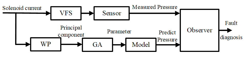
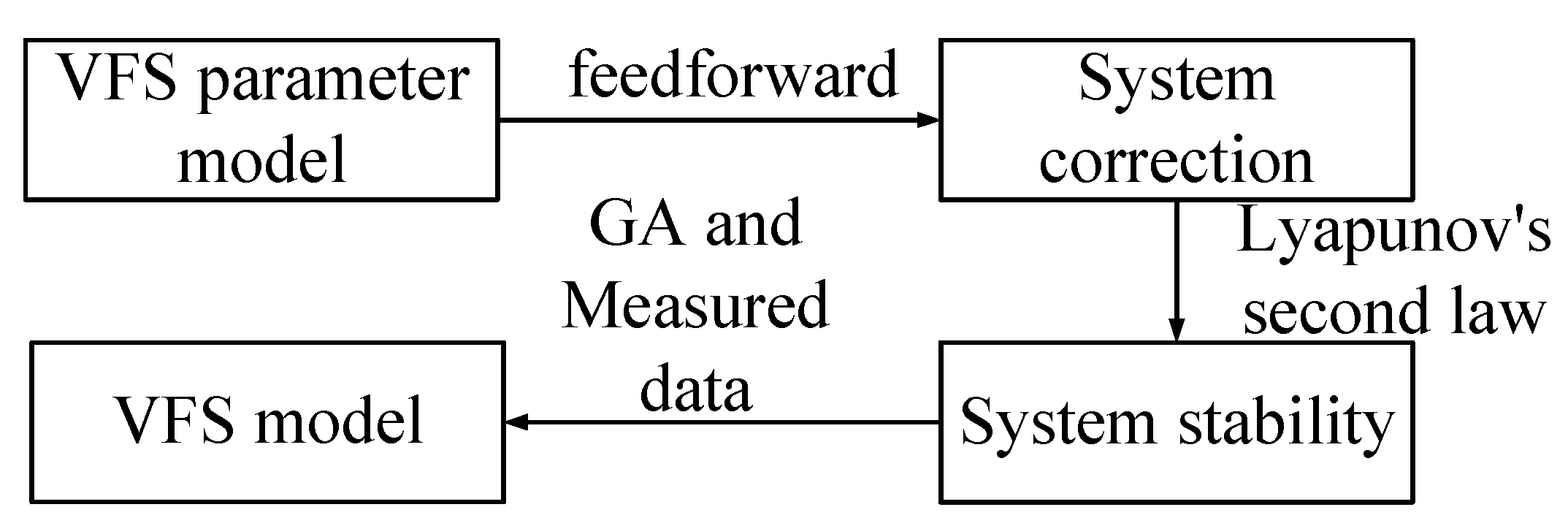
Based on the working principle of solenoid valves, this article establishes a solenoid valve system model, designs an input feedforward system to correct the first-order time lag effect of the sensor, and then use a genetic algorithm combined with the output big data of the actual sensor to identify the model parameters. By using the established model, the fault observer of an actual sensor is designed. The output of the fault observer is proven under different kinds of sensor faults about which enterprises are concerned at present. The system block diagram of fault diagnosis and identification is shown in Figure 1.
2. Modeling the Clutch Pressure System
2.1. Establishment of Mathematical Model
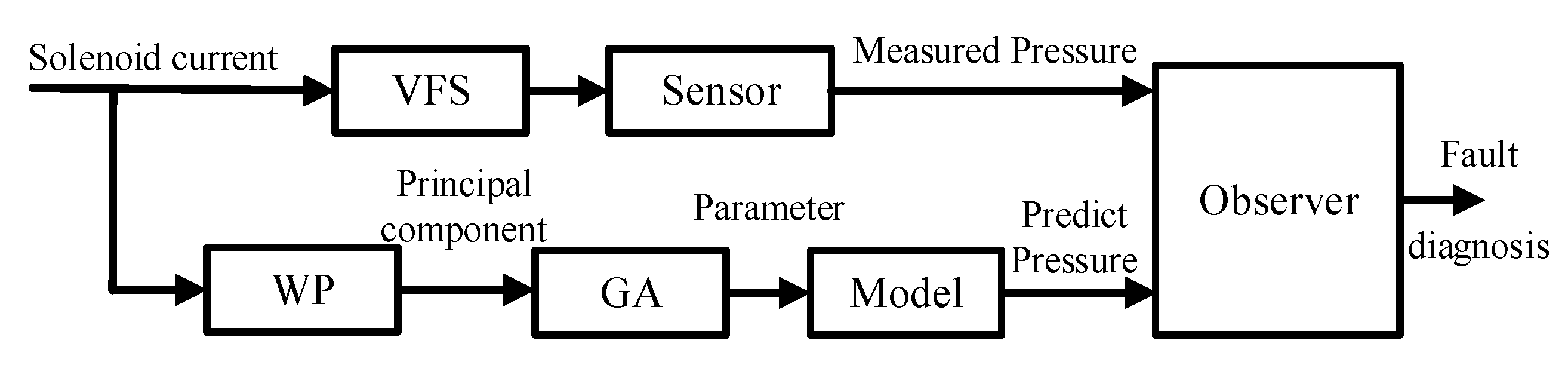
The clutch pressure system of Dual Clutch Transmission (DCT) is composed of a VFS (variable force solenoid) valve, a two-position three-way slide valve, and a corresponding oil hydraulic circuit. The structure diagram is shown in Figure 2:
The oil chamber III is directly connected to the oil inlet, and the oil chamber IV is connected to the clutch pressure plate. As the two-position, three-way valve piston moves to the right, the oil return circuit is gradually sealed and the oil inlet circuit is gradually opened. The pressure oil flows from chamber III into chamber IV. In practical work, the leakage flow in a VFS is approximately zero.
From relevant knowledge of fluid mechanics [9] and hydraulic control system [10], the flow rate into the hydraulic cylinder can be obtained so that the flow rate and pressure from the III chamber to the IV chamber meet the throttling Formula (1):
where is the flow rate, is the flow coefficient of slide valve, is the port area gradient of the slide valve, is the valve core moving distance, is the hydraulic oil density, and is the chamber pressure difference of both sides.
Assuming that the back-flow pressure is zero, the hydraulic oil is an incompressible fluid, and the throttle orifice is symmetric and matched, the flow in each chamber can be obtained as:
Formula (2) can be written as:
The telescopic distance of the VFS valve is about 1.8 mm. It can be considered that it works in a small range near the operating point; as such:
Formula (5) becomes:
Expanding Formula (5) into a second-order Taylor series results in:
The original working point of the VFS valve can be approximated to zero, that is:
then:
where is the flow gain of the slide valve and is the flow pressure coefficient of the spool valve.
Then, Formula (11) becomes:
The pressure in the orifice can be approximately proportional to its orifice area:
From Formulas (3) and (4):
From Formula (14):
where
Due to:
Thus, Formula (15) can be approximated as:
Based on Newton’s second theorem, the force balance equation of the slide valve can be established as:
where is the quality of the solenoid armature, is partial damping coefficient in the solenoid valve, is elastic coefficient of the return spring in the electromagnet, is the displacement of the servo valve core, is the electromagnetic force on the system, and is the force area of the piston of the slide valve
Combining the practical working environment of the slide valve and Formulas (12), (16), (17) results in:
where is the vacuum permeability, is the magnetic flux area, is the winding radius, and is the energizing current of the solenoid valve.
A Laplace transform of Formula (18) gives:
where a, b, and c are parameters that are to be determined.
2.2. Input Feedforward Design
2.2.1. Input Feedforward
Considering that a sensor has a certain delay effect, it is functionally similar to an inertial link [11], so a feedforward system was designed to compensate for that offset:
The zero point of the system was designed according to the time coefficient of the sensor inertia link to correct the system performance.
Formula (19) can be converted into a state space equation:
where , , .
The observability and controllability of system are proven as follows:
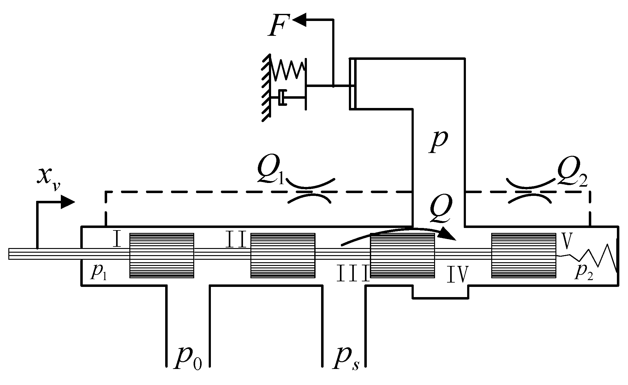
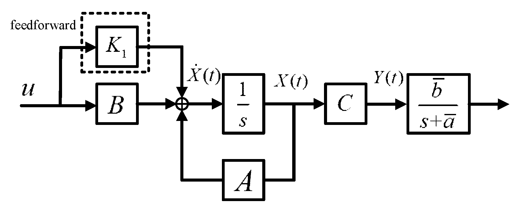
The block diagram of the input feedforward system is shown in Figure 3.
With input feedforward, the system state space equation becomes:
where .
It can be seen from the formula that the input feedforward does not change the matrix, so the system observability remains unchanged, and the controllability is proven as follows:
Thus, the system can be controlled.
Therefore, by introducing input feedforward into the original system, the controllability and observability of the system remain unchanged.
At this point, the system transfer function is:
If , then the zero of the system can be configured and the gain of the transmission function can be adjusted to correct the inertial link of the sensor.
2.2.2. Proof of System Stability
Lyapunov’s second law can be used to prove the stability of the system.
When the system input is zero, the state space equation can be expanded to:
Select:
Then:
According to Lyapunov’s second law, if system stability requires , , then it requires and .
Figure 4 shows the steps of the modeling process.
2.3. Model Parameter Identification Based on GA Algorithm
2.3.1. Input Signal Principal Component Extraction Based on Wavelet Packet Transform
Wavelet packet analysis is a kind of effective signal processing theory. The approximate coefficients and detail coefficients of layer 1 are obtained by filtering the original signal through a low pass filter and a high pass filter, respectively. By filtering the approximate coefficients and detail coefficients of layer 1, the approximate coefficients and detail coefficients of layer 2 are gained. The process is then continued until the requirement is met. The signal can be expressed as:
where is the conjugate matrix of the low pass filter and is the conjugate matrix of the high pass filter. The original signal can be expressed as .
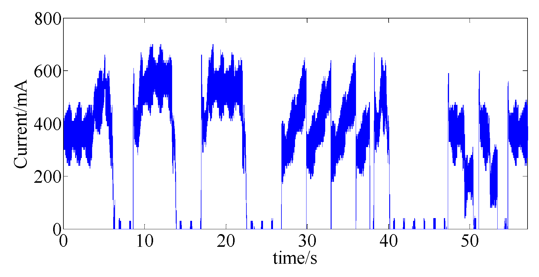
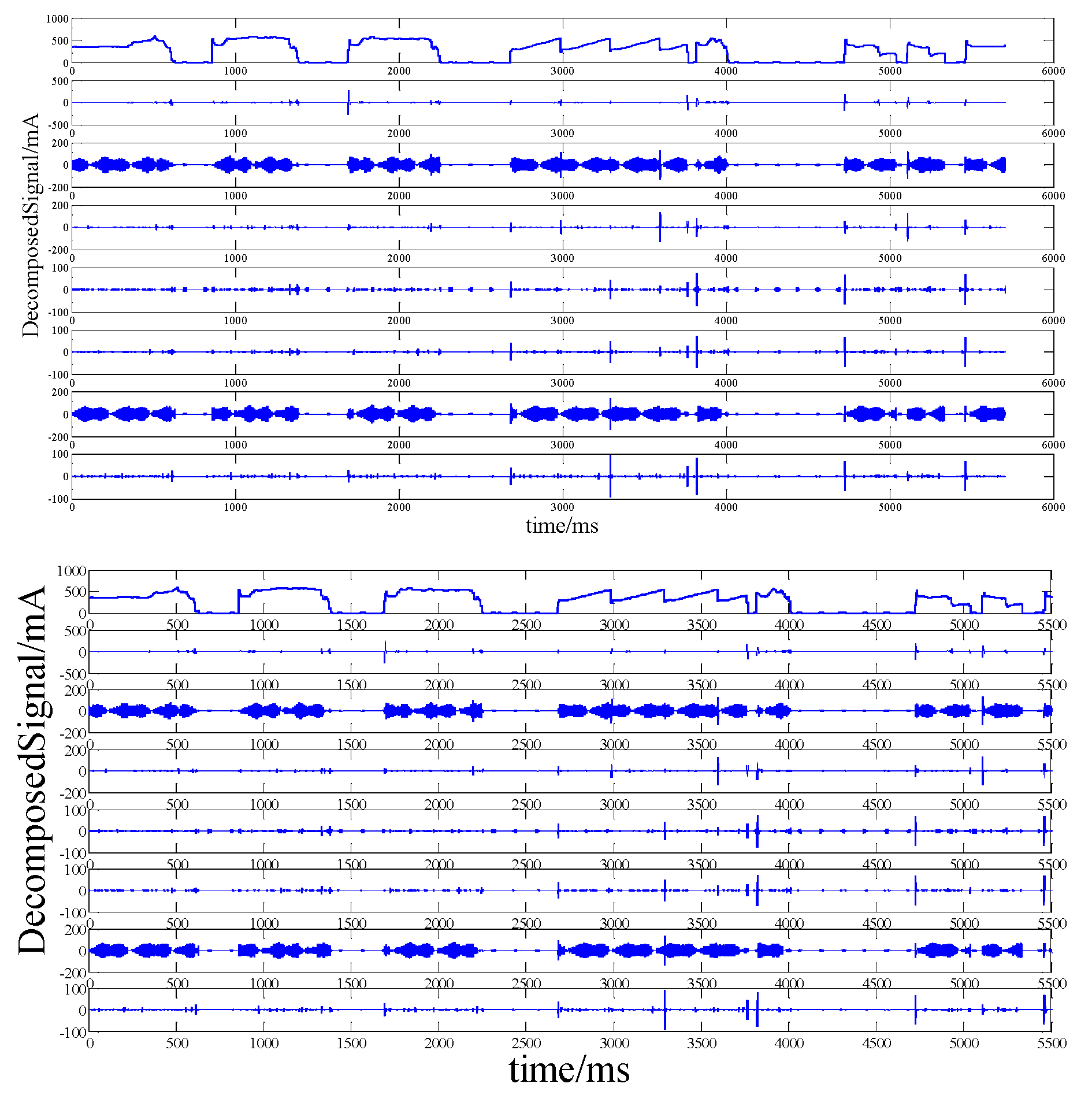
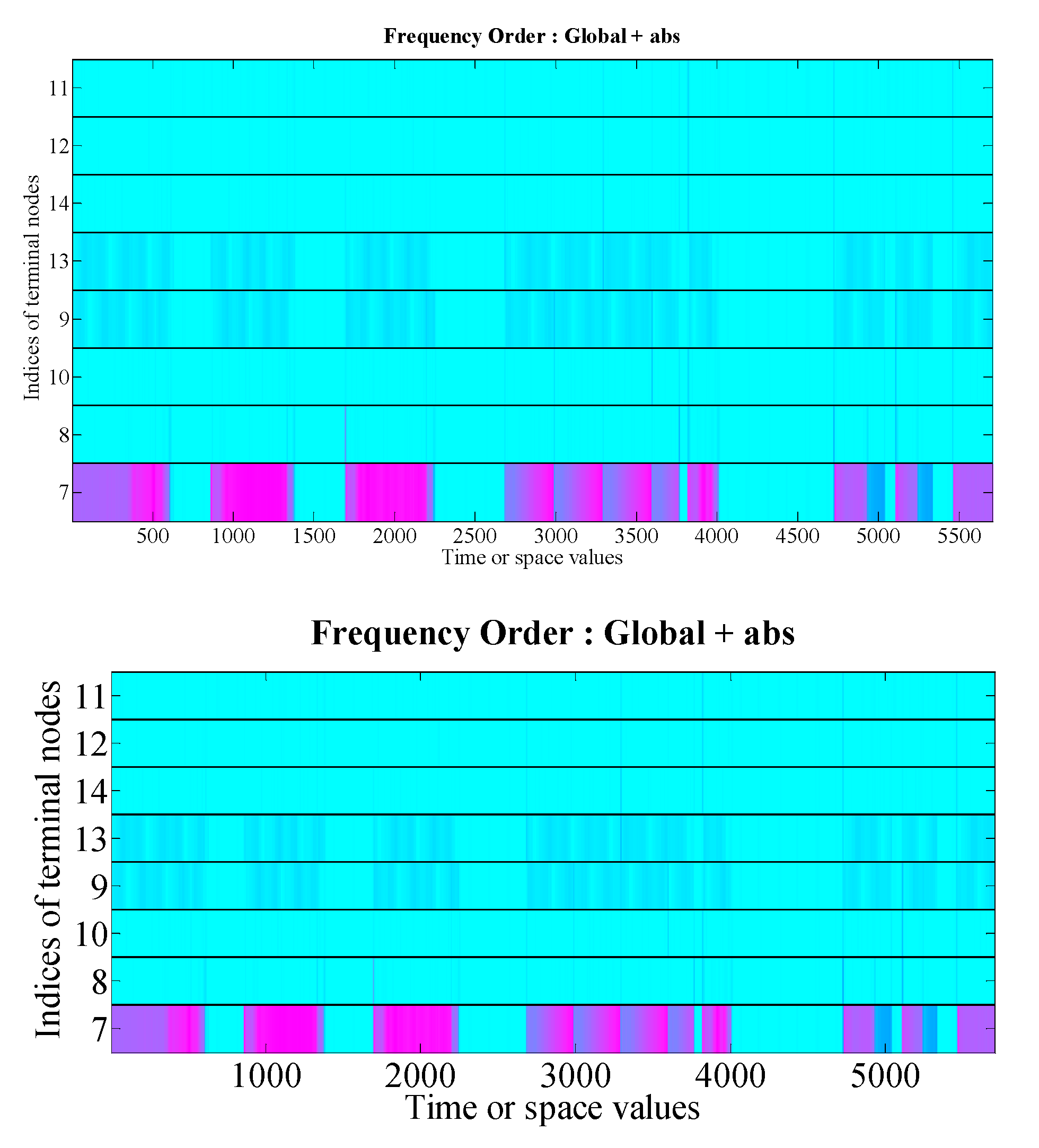
Here, wavelet packet analysis was performed on the solenoid valve current signals to extract principal component information. The data used for identification were collected when the throttle pedal was at its 30% opening value. The solenoid valve input current signal is shown in Figure 5. The wavelet packet decomposition of the current signal is shown in Figure 6
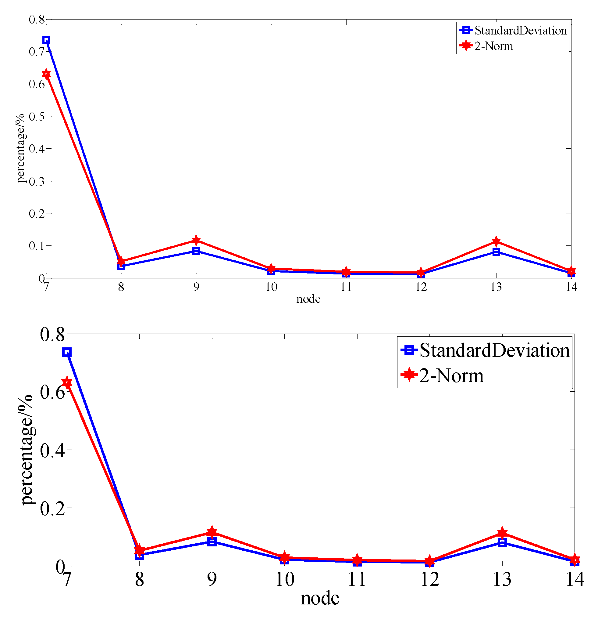
The root mean square value and two-norm value of all eight-layer wavelet signals that were decomposed by the wavelet packet were obtained, and the ratio of the wavelet packet signal in each layer to the original signal was calculated according to Formulas (34) and (35). The result is shown in Figure 6.
where is the two-norm of the layer signal.
where is the layer signal’s standard deviation.
Figure 7 shows the signals, except for the first layers are all high-frequency signals, which are different from the frequency of the control signal and closer to the noise. Figure 7 also shows the standard deviation and two-norm values of all the layers. The seventh layer signal’s deviation and its two-norm value were 63% and 73% of the original signal, respectively. As shown in Figure 8, the energy of the original signal was also mainly concentrated in the signal of layer 7, so the signal of layer 7 was selected as the input control signal.
2.3.2. Genetic Algorithm
Through feedforward correction, the system could be approximated to a second-order system with three parameters. The parameters of the model could be determined by using the data that were measured by the actual sensor and the genetic algorithm.
A genetic algorithm is a kind of randomized search algorithm that uses natural selection and natural genetic mechanisms for reference. A genetic algorithm simulates the phenomenon of reproduction, crossover, and gene mutation in the process of natural selection and natural heredity. This algorithm keeps a group of candidate solutions in each iteration, selects the better individuals from the solution group according to a certain index, and uses genetic operators (selection, crossover and mutation) to combine these individuals to generate a new generation of candidate solution groups. This process can be repeated until a certain income meet the requirements.
A genetic algorithm is composed of the following four parts:
- (1)
- Coding (generating initial population).
- (2)
- Fitness function.
- (3)
- Genetic operator (selection, crossover, and mutation).
- (4)
- Operation parameters.
The coding of the target is the first step of the algorithm, then the fitness function is used to calculate the fitness value for selecting the better individuals. After the selection, crossover, and mutation processes, a new population is generated. The iteration of the algorithm does not stop until the target meets the requirement.
In this paper, the genetic algorithm and data measured from actual sensor were used to identify the parameters of the solenoid valve model. Binary code was chosen, the original population number was set as 30, the genetic algebra was set as 300, and the fitness function was selected as the root mean square error of the actual sensor output and the model output of each generation. The fitness function is shown in Formula (36):
where is the model output of the generation and is the actual sensor output.
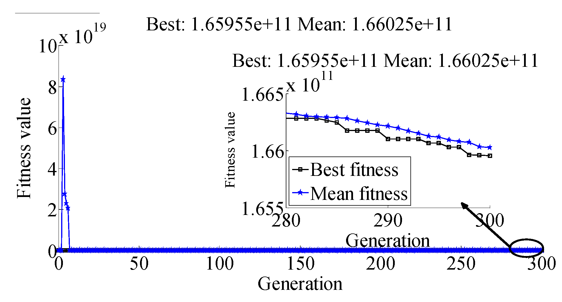
As shown in Figure 9, the best and average fitness values of the system for each generation were declined. The best fitness function value after 300 generations of algorithm iteration was about 1.66e + 11. The model parameters were selected at this time as , , and .
According to the result of stability analysis, the model that was optimized by the genetic algorithm was stable.
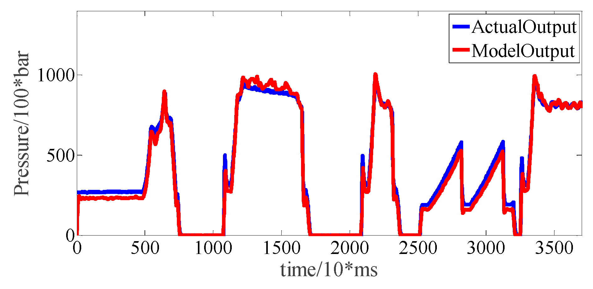
The data that were used for pressure tracking were collected when the throttle was at 50% of its opening value. Layer 7 of the control current of the solenoid valve was tracked. The output of the model was compared with the actual pressure. The result is shown in Figure 10. It can be seen from the figure that the identified system had a high tracking accuracy for the original signal.
3. Fault Observer
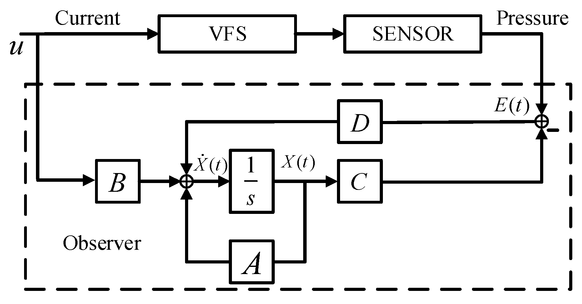
The model was used to design a fault observer of the original solenoid valve system. The structure diagram of the fault observer is shown in Figure 11.
The system equation is:
The observer was designed as:
The state error was defined as:
The output error was defined as:
When the sensor fails:
where is the fault vector. In the case that a certain sensor fails, is the fault manifestation.
Solve Equation (44):
Simplify:
where and is the Scalar constant. If the fault type is n-order fault, Formula (48) is converted to:
where is the order derivative of the fault signal.
Output error:
According to Formula (50), the form of output error is determined by the form and the order derivative of the fault signal. Different fault forms have specific output results. By monitoring the state error and output error, system fault diagnosis can be completed. The output error and state error are close to zero when no component fails.
4. Verification
4.1. Constant Output Fault
In this stage, three kinds of sensor faults modes—0 V constant output, 3 V constant output, and 5 V constant output—were selected. The driving conditions of an automobile are classified into four categories: the launching, upshift, fixed gear driving, and downshift conditions. This model assumes that all driving conditions have been covered.
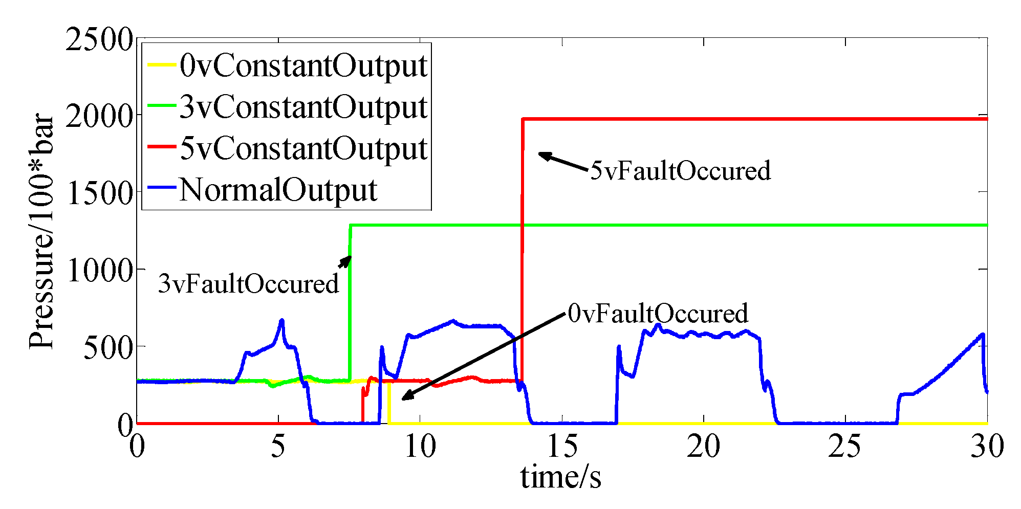
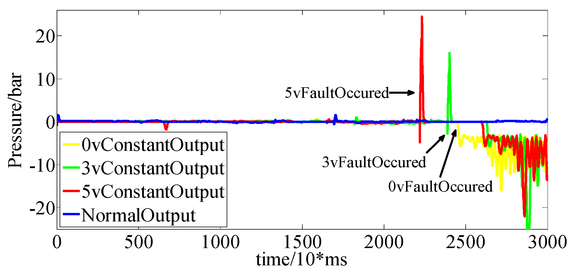
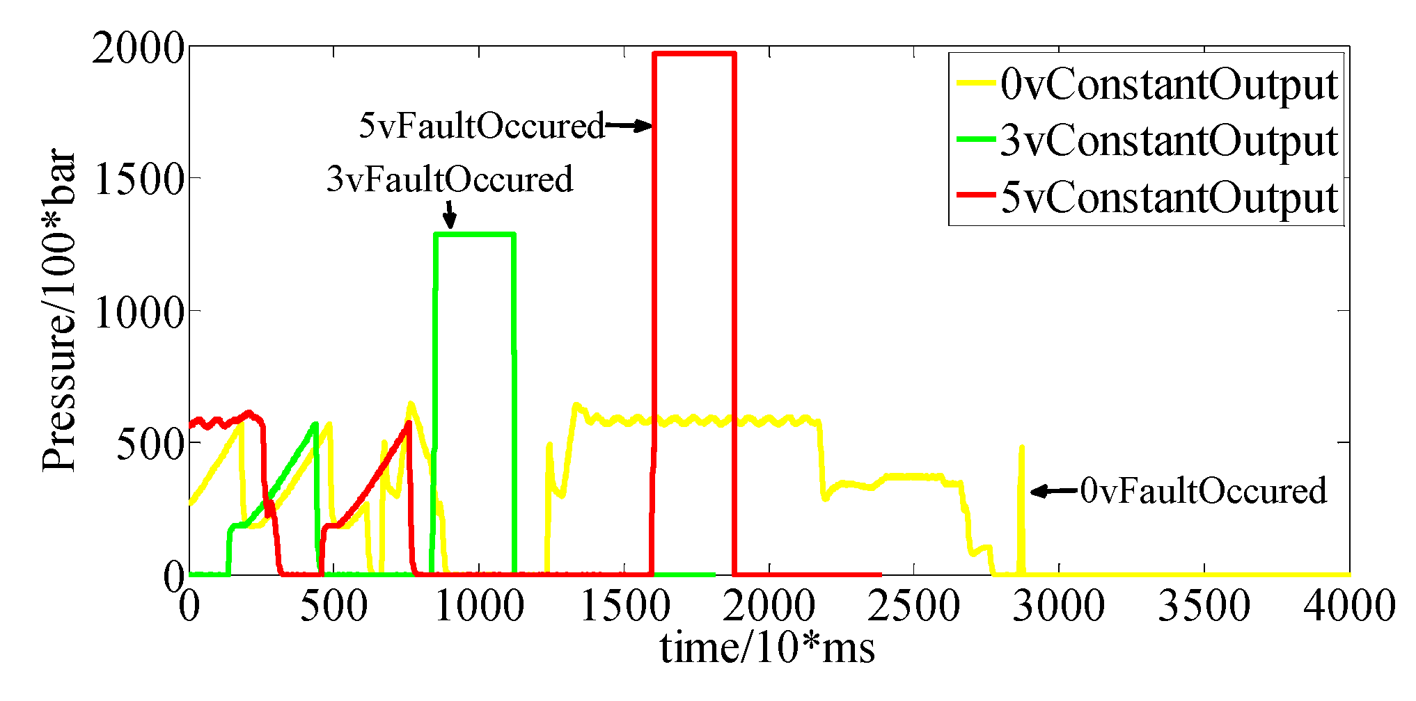
In the launch condition, three kinds of failure are set. The output signal of the clutch pressure sensor is as shown in Figure 11, and the output of fault observer is as shown in Figure 12.
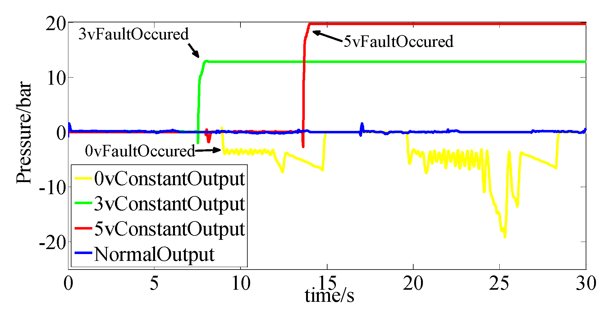
As shown in Figure 12, the outputs of sensor changed to 0, 3 and 5 V at certain time points under launch condition. The fault observer’s output also varied, as shown in Figure 13. According to the results, the form of the fault observer’s output varied according to different kinds of faults. When there was no fault in the system (the blue line in the figure), the output value fluctuated near 0, indicating that there was no big deviation between the output of the observer and the actual output.
When the sensor had a 0 V constant value fault (yellow line in the figure), the fault observer output a signal with a negative amplitude, and the trend of the output was closed to the control current of the solenoid valve. Because the model predicted the clutch pressure value according to the control current of the solenoid valve but the output of the sensor was 0, so the output form of the fault observer followed the difference between the actual sensor and the model system.
When a 3 V constant output fault occurred in the system (green line in the figure), the fault observer output an observation result with a positive amplitude, and the form was consistent with the fault shape of the sensor.
From the system point of view, at this time, the sensor output is a constant non-zero value and feeds back to the controller of the solenoid. The controller of the solenoid generates new control rate according to this received signal. Because the signal is non-zero and constant, the controller’s output is surely affected by this value. From the mathematical point of view, the form of fault is constant value fault and the first and above order derivative of fault signal are all zero, so Formula (50) becomes:
Thus, the output of the fault observer and the sensor fault have the same trend.
When a 5 V constant output fault occurred in the system (red line in the figure), the fault observer output an observation result with a positive amplitude, and the form was consistent with the fault shape of the sensor. The cause analysis was consistent with the 3 V constant output fault. As shown in Figure 13, the observer output of different kinds of faults under different driving conditions was confirmed. The threshold for fault diagnosis could be selected for different conditions. The threshold varied with different kinds of faults. In this paper, the threshold for the normal mode and the 3 V constant output fault could be selected as 5 bar, the thresholds for the 3 and 5 V constant output faults could be selected as 17 bar, and the thresholds for the 0 and 3 V constant output faults could be selected as -5 bar. As shown in the Figure 13, the fault was able to be well-diagnosed.
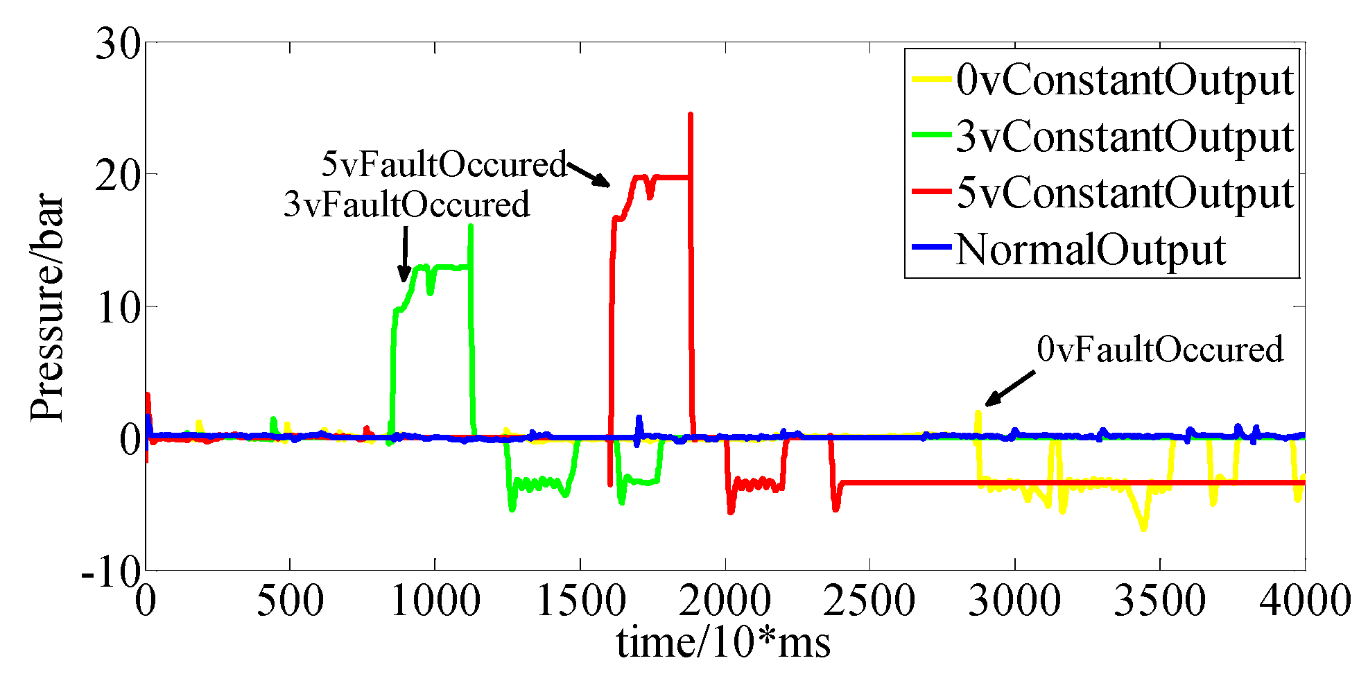
In the upshift condition, three kinds of faults are set. The output signal of the clutch pressure sensor is as shown in Figure 14, and the output of the fault observer is as shown in Figure 15. The threshold could be selected accordingly.
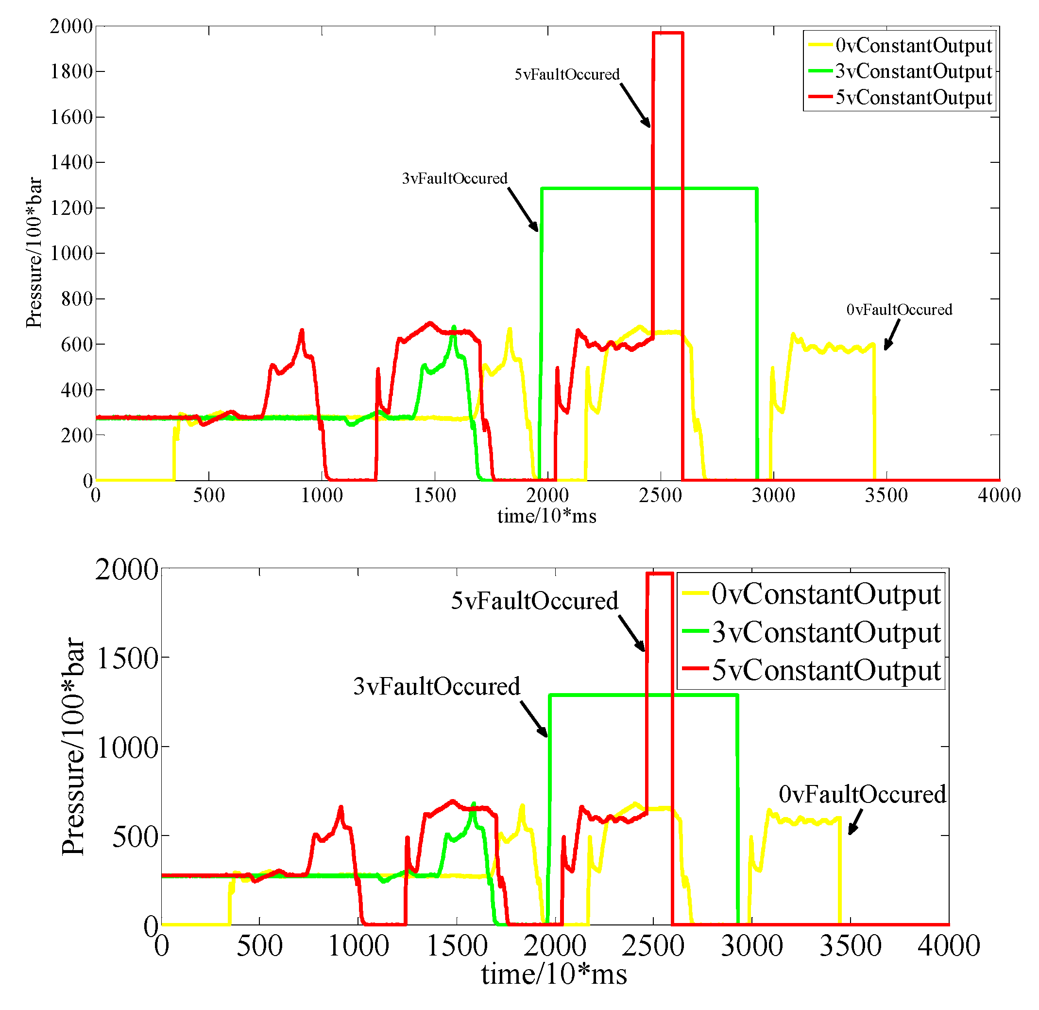
In the fixed gear condition, three kinds of faults are set. The output signals of the clutch pressure sensor are as shown in Figure 16, and the output of the fault observer is as shown in Figure 17. The threshold can be selected accordingly.
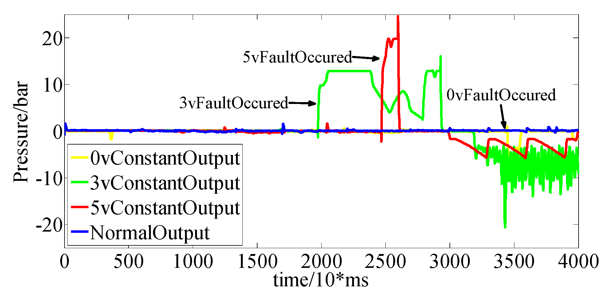
In the downshift condition, three kinds of faults are set. The output signal of the clutch pressure sensor is as shown in Figure 18, and the output of the fault observer is as shown in Figure 19. The threshold can be selected accordingly.
The observer’s output of three kinds of faults under the upshift, fixed gear and downshift conditions are synthetically considered and the result are consistent with that in the launch stage. Because it was impossible to completely shield all the fault-tolerant control strategies and replacement strategies of mature industrial production when collecting the actual sensor signals, the output signals of the sensors were not always consistent under some driving conditions when doing the test, but the diagnosis results were not affected. According to Figure 14, Figure 15, Figure 16, Figure 17, Figure 18 and Figure 19, the output of the fault observer varied according to different faults, as expected under different driving conditions.
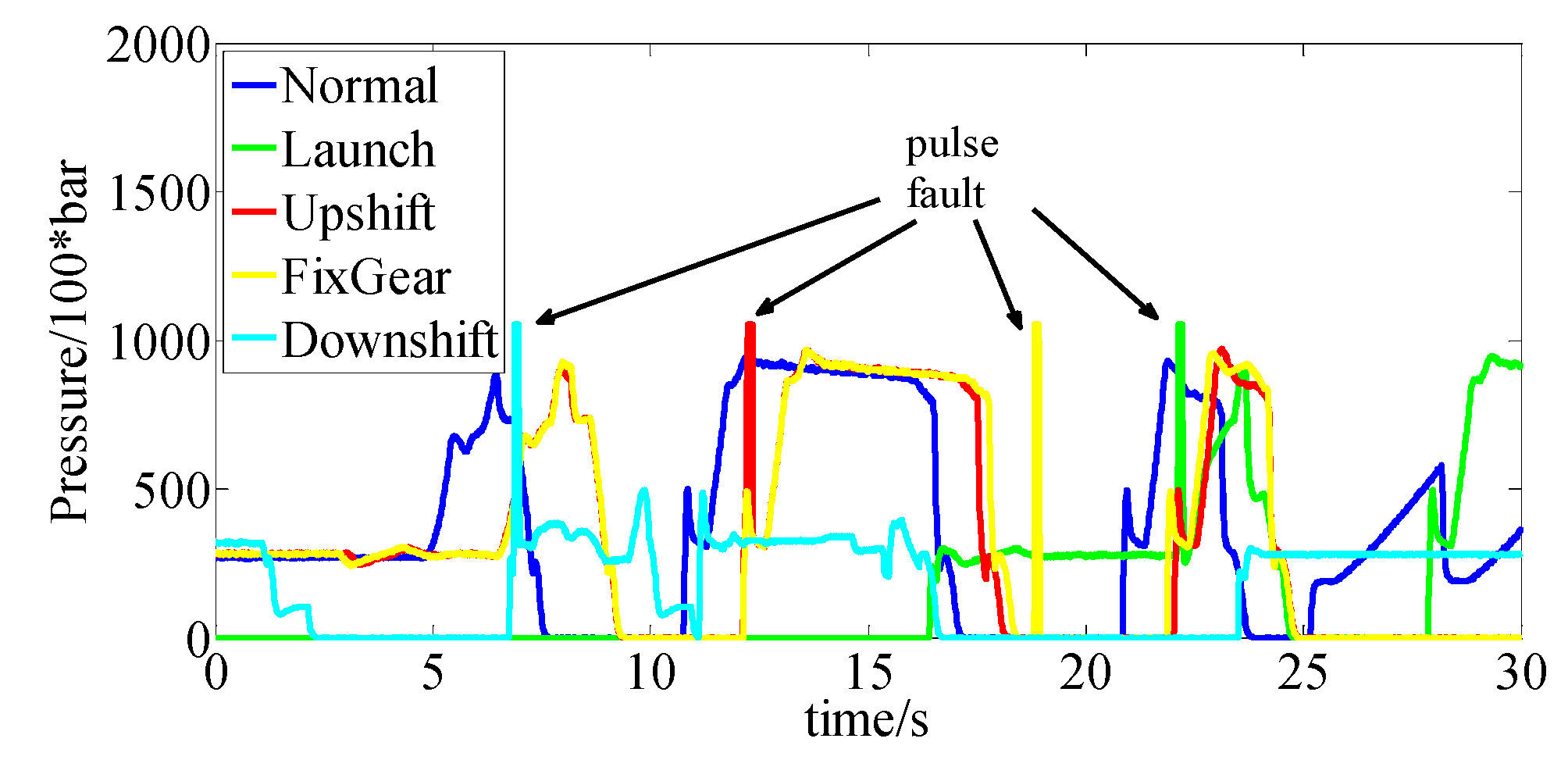
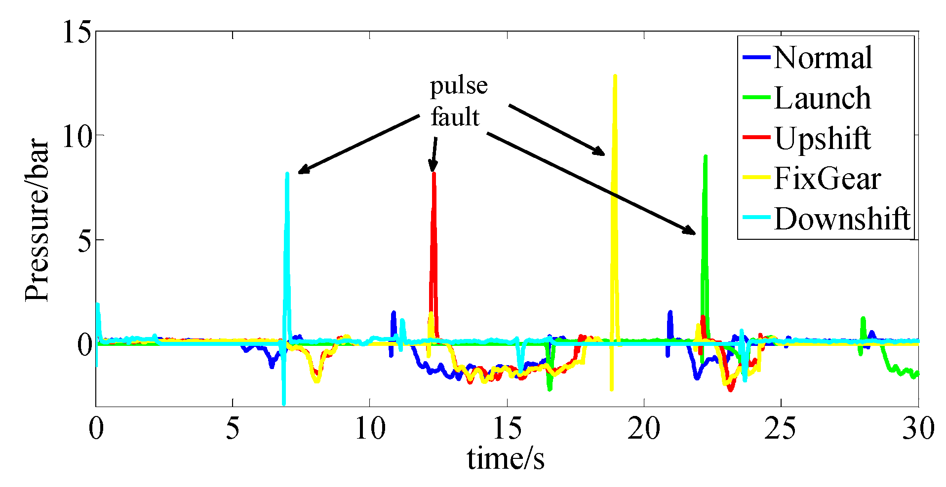
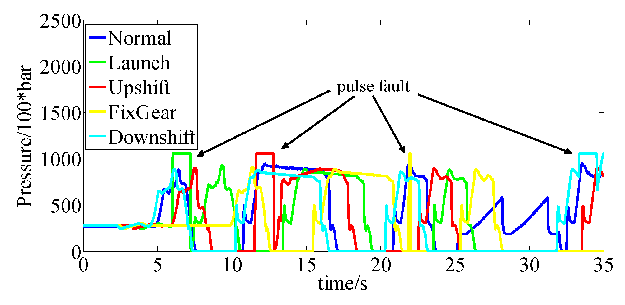
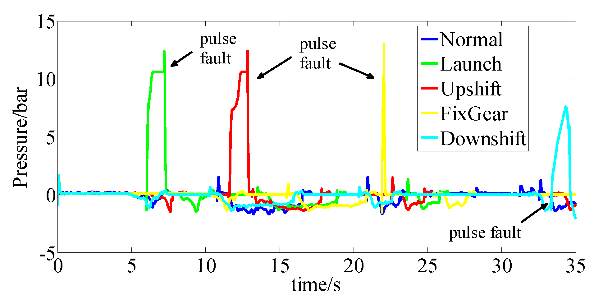
4.2. Pulse Fault
In this stage, the pulse fault was tested. A pulse fault is divided into two kinds; the first one lasts for 0.1 s, and the other is lasts for 1 s, and the enterprise is concerned with both. The amplitude is a certain value. The driving conditions of an automobile are classified into four categories: the launching, upshift, fixed gear driving and downshift conditions. This model assumes that all driving conditions have been covered.
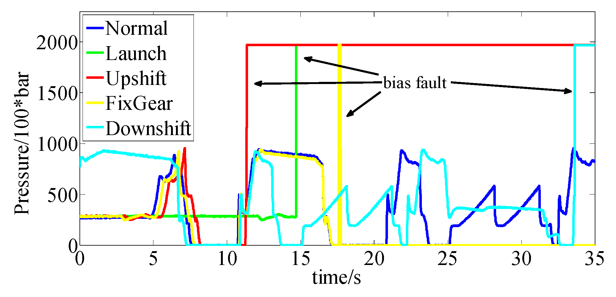
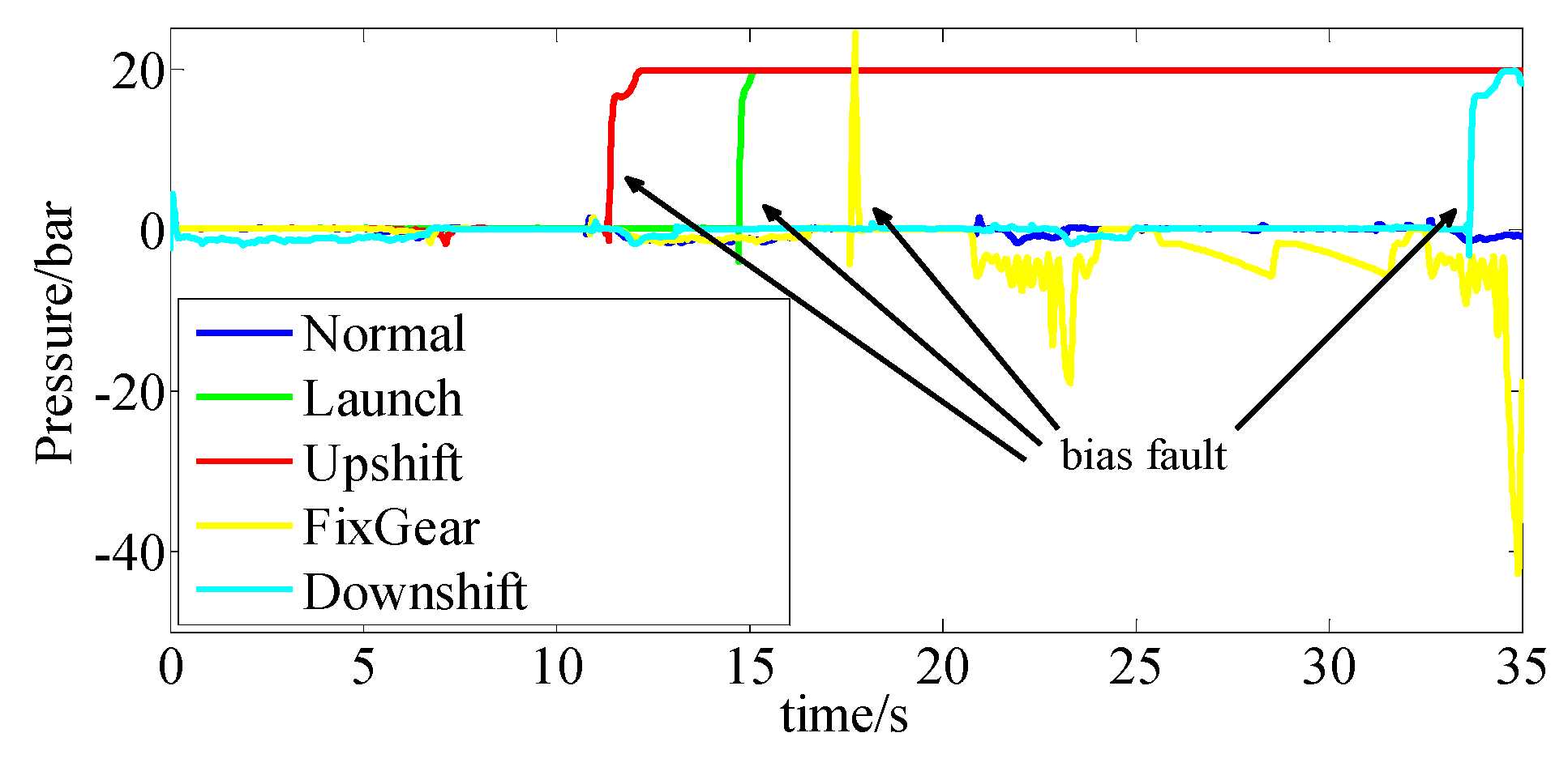
4.3. Bias Fault
In this stage, the bias fault was tested. Bias fault is a common fault that deviates in sensor output. The driving conditions of an automobile are classified into four categories: the launching, upshift, fixed gear driving, and downshift conditions. This model assumes that all driving conditions have been covered.
5. Conclusions
This paper proposed a fault diagnosis method for the pressure sensor of DCT. Firstly, the model of a VFS valve was established, and then the first-order inertial link of the sensor was corrected with the design of a feed-forward system. The parameters of the model were identified by using the actual sensor data of transmission and a GA algorithm. Then, the fault observer was designed by using the identified model. From the theoretical point of view, different types of faults have different kinds of observation outputs. Here, the form of observation output varied with the form of fault. In the verification stage, the fault observer outputs were verified by the measured fault signals of the pressure sensor. Constant output faults of 0, 3, and 5 V, the pulse fault, and the bias fault, all of which the enterprise is concerned by, are generated. The results showed that the designed fault observer had the expected diagnosis effect and function, can diagnose different types of faults, and can output specific results according to different types of faults. By identifying fault types according to the fault observer output, a fault diagnosis method has established, and this lays a foundation for later fault-tolerant control.
Author Contributions
Conceptualization, G.W. and Z.L.; methodology, Z.L.; validation, G.W.; project administration, G.W.; funding acquisition, G.W. All authors have read and agreed to the published version of the manuscript.
Funding
This research was funded by National Natural Science Foundation, grant number is U1764259.
Conflicts of Interest
The authors declare no conflict of interest.
References
- Lucke, M.; Stief, A.; Chioua, M.; Ottewill, J.R.; Thornhill, N.F. Fault detection and identification combining process measurements and statistical alarms. Control Eng. Pract. 2020, 94, 104195. [Google Scholar] [CrossRef]
- Choi, U.M.; Lee, J.S.; Blaabjerg, F.; Lee, K.B. Open-Circuit Fault Diagnosis and Fault-Tolerant Control for a Grid-Connected NPC Inverter. IEEE Trans. Power Electron. 2016, 31, 7234–7247. [Google Scholar] [CrossRef]
- Jaradat, M.A.; Langari, R. A hybrid intelligent system for fault detection and sensor fusion. Appl. Soft Comput. 2009, 9, 415–422. [Google Scholar] [CrossRef]
- Cui, X.; Wang, S.; Li, T.; Shi, J. System Reliability Assessment Based on Energy Dissipation: Modeling and Application in Electro-Hydrostatic Actuation System. Energy Fuels 2019, 12, 3275. [Google Scholar] [CrossRef] [Green Version]
- Ni, S.X.; Zhang, Y.F.; Yi, H.; Liang, X.F. Intelligent Fault Diagnosis Method Based on Fault Tree. J. Shanghai Jiaotong Univ. 2008, 42, 1372–1375. [Google Scholar]
- Barik, M.A.; Gargoom, A.; Mahmud, M.A.; Haque, M.E.; Al-Khalidi, H.; Oo, A.M. A Decentralized Fault Detection Technique for Detecting Single Phase to Ground Faults in Power Distribution Systems with Resonant Grounding. IEEE Trans. Power Deliv. 2018, 33, 2462–2473. [Google Scholar] [CrossRef]
- Lei, Y.; Yang, B.; Du, Z.; Lu, N. Deep Transfer Diagnosis Method for Machinery in Big Data Era. J. Mech. Eng. 2019, 55, 1–8. [Google Scholar] [CrossRef]
- Sylvain, V.; Teodor, T.; Abdessamad, K. Fault detection and identification with a new feature selection based on mutual information. J. Process Control 2008, 18, 479–490. [Google Scholar]
- Yu, P. Hydrodynamics, 2nd ed.; Science Press: Beijing, China, 2016; pp. 53–74. [Google Scholar]
- Li, H. Hydraulic Control System, 1st ed.; National Defense Industry Press: Beijing, China, 1990; pp. 53–70. [Google Scholar]
- Eriksson, L.; Nielsen, L. Modeling and Control of Engines and Drivelines, 1st ed.; Wiley: Hoboken, NJ, USA, 2014. [Google Scholar]
Figure 1.
Block diagram of fault diagnosis system.

Figure 2.
VFS (variable force solenoid) valve structure diagram.

Figure 3.
Input feedforward system block diagram.

Figure 4.
Steps of modeling.

Figure 5.
Control current of a solenoid valve.

Figure 6.
Schematic diagram of wavelet packet signal decomposition.

Figure 7.
Standard deviation and two-norm of each data node.

Figure 8.
Data analysis of each data node.

Figure 9.
Fitness value of each generation.

Figure 10.
Pressure tracking.

Figure 11.
Diagram of the fault observer.

Figure 12.
Sensor output under launch condition.

Figure 13.
Observer output under launch condition.

Figure 14.
Sensor output under upshift condition.

Figure 15.
Observer output under upshift condition.

Figure 16.
Sensor output under the fixed gear condition.

Figure 17.
Observer output under the fixed gear condition.

Figure 18.
Sensor output under the downshift condition.

Figure 19.
Observer output under the downshift condition.

Figure 20.
0.1 s pulse fault sensor.

Figure 21.
Observer output of the 0.1 s pulse fault sensor.

Figure 22.
1 s pulse fault sensor.

Figure 23.
Observer output of 1 s pulse fault sensor.

Figure 24.
Bias fault sensor.

Figure 25.
Observer output of bias fault sensor.

© 2020 by the authors. Licensee MDPI, Basel, Switzerland. This article is an open access article distributed under the terms and conditions of the Creative Commons Attribution (CC BY) license (http://creativecommons.org/licenses/by/4.0/).
Share and Cite
MDPI and ACS Style
Lv, Z.; Wu, G. A Novel Method for Clutch Pressure Sensor Fault Diagnosis. Vehicles 2020, 2, 191-209. https://0-doi-org.brum.beds.ac.uk/10.3390/vehicles2010011
AMA Style
Lv Z, Wu G. A Novel Method for Clutch Pressure Sensor Fault Diagnosis. Vehicles. 2020; 2(1):191-209. https://0-doi-org.brum.beds.ac.uk/10.3390/vehicles2010011
Chicago/Turabian StyleLv, Zhichao, and Guangqiang Wu. 2020. "A Novel Method for Clutch Pressure Sensor Fault Diagnosis" Vehicles 2, no. 1: 191-209. https://0-doi-org.brum.beds.ac.uk/10.3390/vehicles2010011