Cooperative Highway Lane Merge of Connected Vehicles Using Nonlinear Model Predictive Optimal Controller


1
Caterpillar Inc., Mossville, IL 61522, USA
2
Mechanical Engineering, University of Illinois at Chicago, Chicago, IL 60607, USA
*
Author to whom correspondence should be addressed.
Vehicles 2020, 2(2), 249-266; https://0-doi-org.brum.beds.ac.uk/10.3390/vehicles2020014
Submission received: 16 September 2019
/
Revised: 12 March 2020
/
Accepted: 18 March 2020
/
Published: 25 March 2020
(This article belongs to the Special Issue Autonomous Vehicle Control)
Abstract
:Of all driving functions, one of the critical maneuvers is the lane merge. A cooperative Nonlinear Model Predictive Control (NMPC)-based optimization method for implementing a highway lane merge of two connected autonomous vehicles is presented using solutions obtained by the direct multiple shooting method. A performance criteria cost function, which is a function of the states and inputs of the system, was optimized subject to nonlinear model and maneuver constraints. An optimal formulation was developed and then solved on a receding horizon using direct multiple shooting solutions; this is implemented using an open-source ACADO code. Numerical simulation results were performed in a real-case scenario. The results indicate that the implementation of such a controller is possible in real time, in different highway merge situations.
1. Introduction
Autonomous vehicle technology has been a significant research and development topic in the automotive industry during the last decade. The technologies developed in the automotive industry also has direct applications in the construction, mining, agriculture, marine, and unmanned aerial vehicle (UAV) markets. Despite significant R&D activities and investments in this area that date back three decades, it might still take a few decades before an entirely autonomous self-driving vehicle navigates itself through national highways and congested urban cities [1,2]. The prediction is that by the turn of this decade, a fully autonomous self-driving vehicle will be a part of a typical commute in cities in the United States [3], though it might be in more restricted areas. Regulations and standards [4,5] are released regularly to monitor on-road vehicle automation implementation.
Vehicle automation today is based on advanced sensor technology used to sense the environment [6]. It also depends on fast, reliable vehicle-to-vehicle (V2V) communication and intelligent control schemes (i.e., involving machine learning algorithms) to implement complex maneuvers.
As the number of OEMs that contribute to vehicle automation increases, a variety of driving functionalities are being automated [7]. The list of functionalities not only includes alerting the driver, e.g., lane departure warnings, driver sleepiness warnings, obstacle warnings, and pedestrian detection warnings, but also active controls such as stop-n-go, cruise control, lane-change, self-park, night headlight adaptation, construction zone travel, and many more.
One of the most common and critical maneuvers, among other critical driving maneuvers, involves the highway lane merge. In this maneuver, the vehicle moves from one highway lane to another or from a local merge lane adjacent to the highway to the main highway lane. In order to automate this maneuver, simultaneous control of acceleration, brake, and steering is required. While controlling these inputs, the controller needs to track the road profile, respect the speed limits, and look out for traffic on the highway.
This paper presents a Nonlinear Model Predictive Control (NMPC)-based optimization method for highway merge, respecting certain merge constraints. Using a case study of the Dwight Eisenhower Expressway (I-290) highway merge in Chicago, Illinois, this paper presents simulated results for various scenarios.
Autonomous Vehicle Control
Autonomous vehicle control strategies can be divided into two major categories: longitudinal and lateral. In longitudinal control, methods are designed to control the speed and acceleration of all vehicles involved; lateral control strategies mainly address the steering of vehicles.
Longitudinal control requires the merge (host) and highway (leading and trailing) vehicle speed and acceleration and the difference in distance between the merge and highway vehicles. For a platoon, the first vehicle’s speed and acceleration will be relevant to this control. Both vehicles’ on-board sensors read the speed and acceleration, while the range sensors obtain the difference in the merge and highway vehicles’ distance. Radar is a commonly used sensor (other than vision, LIDAR for such measurements [8]. Two different ways can determine the preceding vehicle’s speed and acceleration. One approach is to derive it indirectly using speed data from the host vehicle and combining it with the speed information provided by the host range sensors of the preceding vehicles. Alternatively, the highway vehicle speed and acceleration are communicated to the merging vehicle using the vehicle-to-vehicle communication (V2V) [9], with a fallback mechanism when the V2V is not reliable [10,11].
Lateral control is mainly concerned with steering related maneuvers. For strategic lateral lane change control, the surrounding vehicle environment is crucial. It not only includes the vehicles present in the current lane but also in adjacent lanes along with their dynamics. Minimizing Overall Braking Induced Lane (MOBIL), a higher level lateral strategic control, evaluates the rules required for lane change during mandatory and optional lane changes [12]. Acceleration trajectory, which follows a trapezoidal profile (other studied profiles include polynomial, circular, and cosine approximation to circular), is desired for giving a good transition time while maintaining the comfort of the driver [13]. Genetic algorithms in an optimal formulation and a Bayesian network were also explored for a multilane highway, to increase highway throughput [14]. For lateral control at the vehicle level, different approaches were discussed [15]. One of the approaches involves presenting the lateral maneuver as a track control, another uses a guidance algorithm for a unified lateral maneuver [16]. Another paper presents an implementation of a nonlinear model-based optimized controller on a two-axis truck, using all the available sensory data [17]. An active steering system based on kinematic and dynamic models was used in simulating path planning steering control [18].
2. Highway Merge Problem
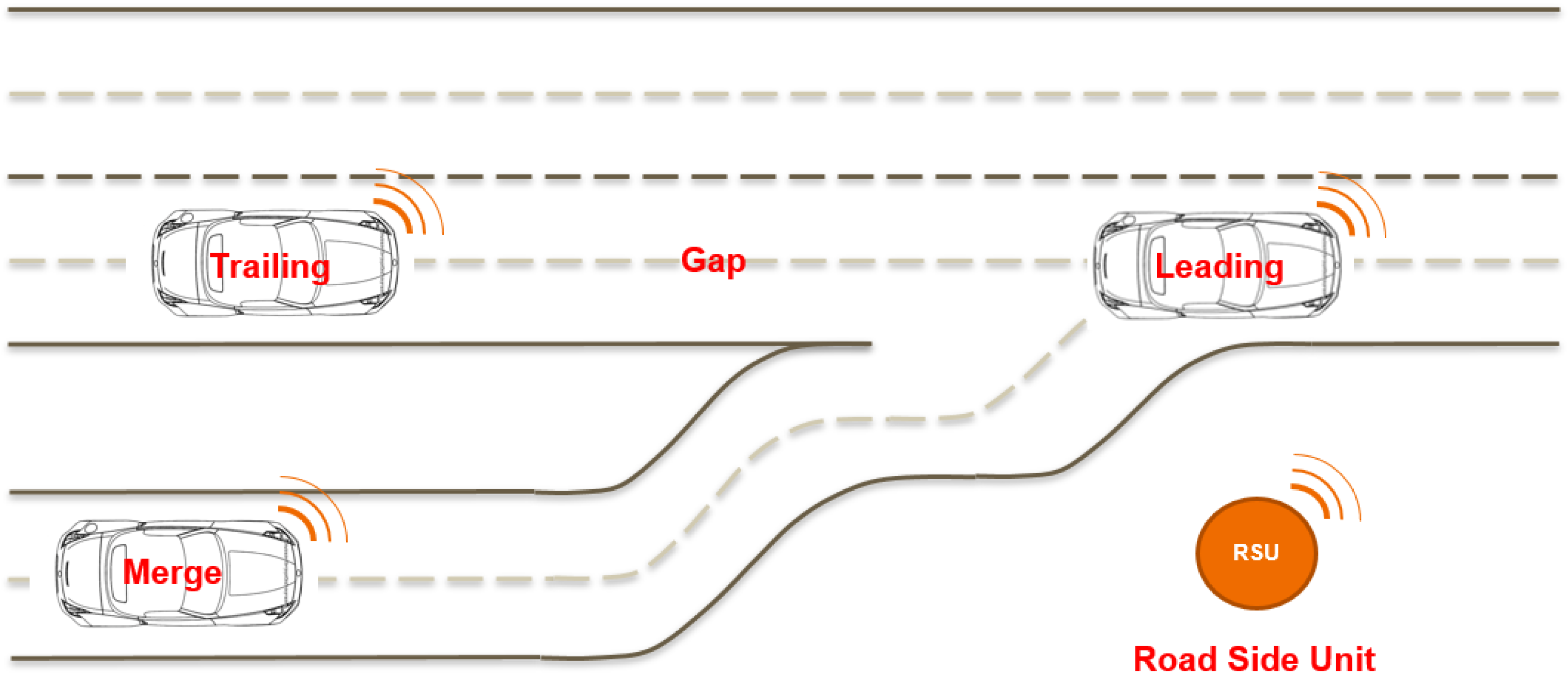
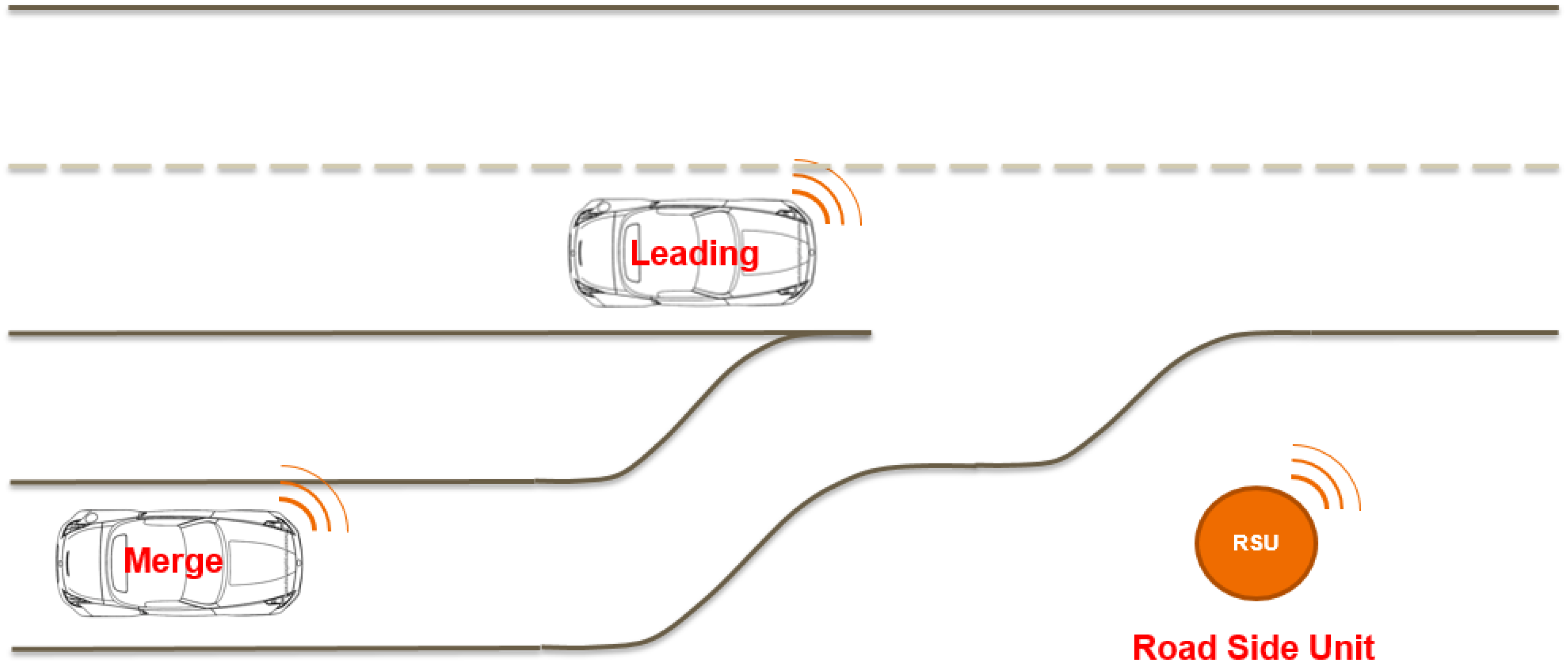
In this maneuver, the merging vehicle is attempting to merge from an adjacent local lane to the main highway lane. In a typical situation, merge happens after finding a gap between two vehicles on the highway, referred to here as lead and trail vehicles. The decision of who will become the lead and trail vehicle during the maneuver can be implemented in two ways: either by a centralized controller on a roadside unit (RSU) guiding the merge and highway vehicles, or by a decentralized controller running in all connected vehicles implementing the highway merge.
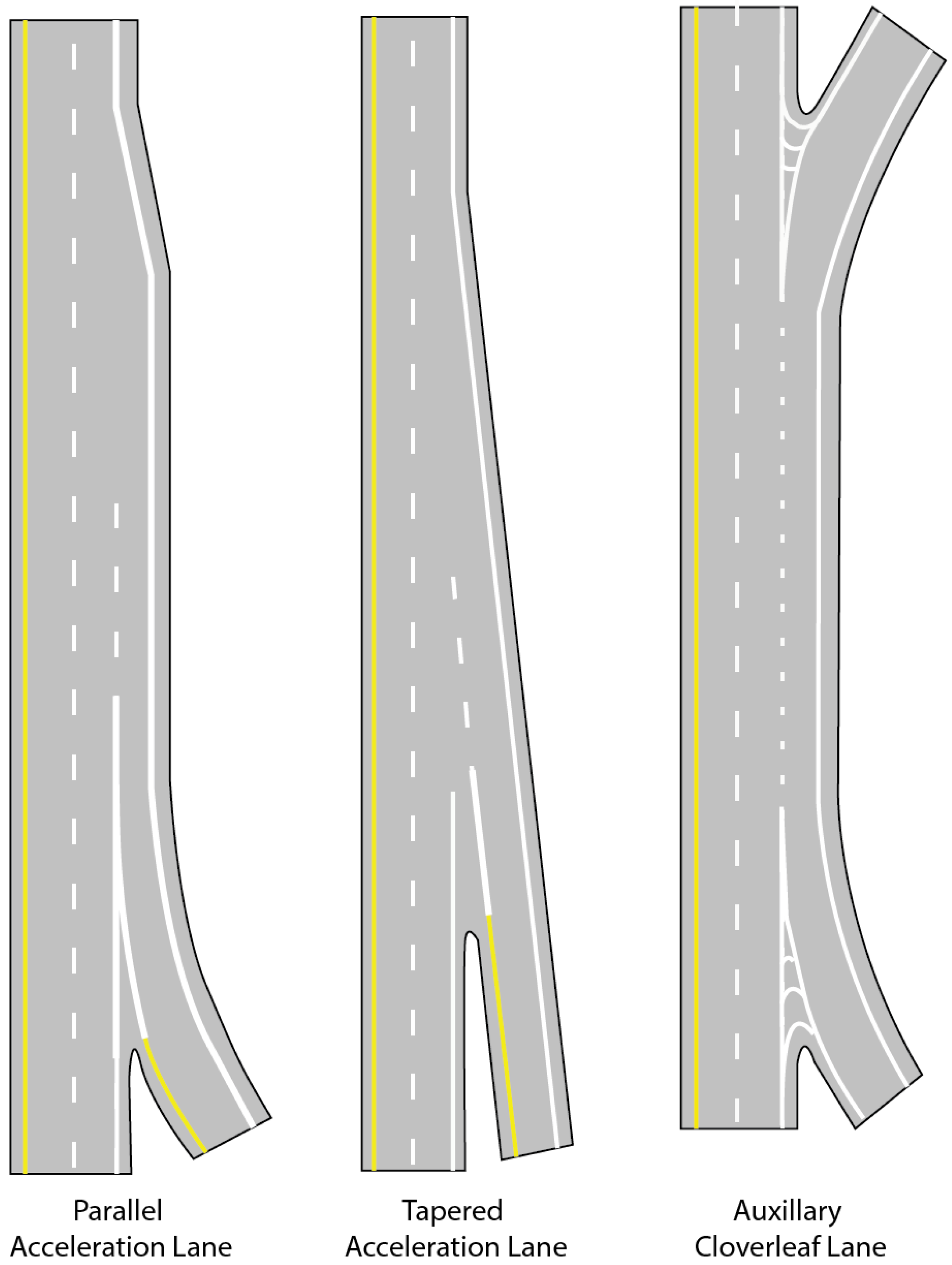
Moreover, the highway merge maneuver will also depend on the configuration of the adjacent local merge lane with respect to the highway lanes. Three types of highway lane merge configuration for the United States are shown in Figure 2. They are referred to as the parallel acceleration lane, tapered acceleration lane, and auxiliary cloverleaf lane. The first type has a parallel lane immediately after the local merge lane. This configuration allows for the vehicles to run in parallel to the highway lane and then implement a lane change. The last one is similar to the parallel lane configuration, as it also allows vehicles to run in parallel to the highway lane and then implement a lane change. The most critical of all highway configurations are tapered lanes, where the vehicle cannot run in parallel to the highway lane but has to immediately join the highway lanes and come up to the designated speed. The tapered lane-type highway merge problem is addressed in this work.
A review of current advances made in connected and automated vehicle research that improves traffic safety by interacting with traffic structures and other connected vehicles is presented in [20]. The model predictive control (MPC)-based merge optimization suggested by [21] searches for a gap in a platoon in the main highway lane. Given the advances made in the V2X, the same strategy can be improved assuming that vehicles are connected and using a better kinematic-based MPC optimization. In [22,23], they used cooperative behavior in their optimization routine; however, the model used in their scheme is a simple particle characterization of the vehicle. A more advanced model of the vehicle could be used, and the optimization scheme redesigned around it, which is the scope of the current work. Most of the simulations were conducted using MATLAB® and its optimization toolbox. The solution was obtained by a rapid generalized minimum residual method (GMRES) method of an associated state-dependent two-point boundary-value problem [22].
The control is optimized over a particular horizon based on the predictions obtained from the model. This limits the use of optimization to implement an online scheme. Most of the solutions presented are offline implementations, rarely applied to a real-time situation. The optimization solution was tested via simulations only. In very few cases, the simulation is compared to the data obtained during a real-time merge process [22,23]. An online scheme can be implemented if the horizon is reduced, thereby decreasing the computation load, but at the cost of decreasing the accuracy of the prediction.
Optimization-Based Strategy
An optimization-based strategy is applied to solve a highway merge problem. Such a strategy adopts a model predictive control (MPC) optimization. The MPC optimization optimizes an objective cost function, usually a function of the states and controls, predicted by a given model. At each sampling time step, it is optimized over a finite time horizon, starting with the current state. The optimized control signal is applied only during the next sample time step of the process. At the next sampling time step, a new prediction of states is computed, and the same optimal control problem is reinitialized using the current sensor reading to obtain a solution for the shifted horizon. The optimal control is subject to input and output constraints.
3. Two-Vehicle Cooperative Highway Lane Merge
3.1. Modeling Assumptions
The mathematical model that is used in this work is formulated from a two-vehicle perspective, shown in Figure 3. The symbols m and h denote the merge and highway (leading) vehicles. The vehicle system state vectors and describe the displacement of merge and highway vehicles, respectively. At initial time interval , state estimates of all vehicles are assumed to be available from the on-board sensors or transmitted between vehicles through V2X communication between vehicles themselves, and between vehicles and infrastructure. Using these current states as initial conditions, the MPC controller predicts the states of the system for the horizon . The optimization problem is solved to determine the optimal control input in order to optimize the cost while satisfying (obeying) the constraints. These optimal control inputs are then given to the low-level vehicle controller used to steer/accelerate/decelerate based on the optimal path. After applying the first control input, the controller algorithm is reinitialized with current states updated as initial conditions. The following assumptions are critical during implementation:
- On-board sensors and sensor fusion techniques are used by each vehicle to uniquely identify its own and other vehicles’ positions and speeds within a specific range of the merging zone;
- The kinematic model is used during the MPC optimization to predict the future evolution of the vehicle system;
- Control decisions to steer, acceleration, and brake are made such that the control objective is minimized and constraints are satisfied.
3.2. Vehicle Kinematic Model and the Vehicle States
The cooperative highway merge model has six states, four states for the merge vehicle described by a subscript m, and two states for the highway vehicle using subscipt h. The states of the merging vehicle model are , where and are longitudinal and lateral displacements, is the vehicle yaw angle, and is the merge vehicle velocity. The merge vehicle inputs are , where a is the acceleration of the vehicle, and is the steering angle of the front wheels. This model is extended to the vehicle in the main highway lane, since the vehicles in the main highway lane are assumed not to make any lateral change, i.e., no steering change is used for the highway vehicles. The highway vehicle longitudinal positions are affected during the merge by acceleration and deceleration. Therefore, the states of these vehicles are , and is the acceleration inputs to highway vehicles. The combined cooperative highway merge model formulation of the merging vehicle in the merge lane and the highway vehicle in the highway lane can be written as follows:
where depends on the steering input to the merging vehicle, as shown in [24].
3.3. Nonlinear Model Predictive Controller
The nonlinear MPC optimization is similar to linear optimization except that the model used in the model predictive control optimization is nonlinear. Similar to standard optimization algorithms, it has an objective cost function plus constraints. Furthermore, in most cases, the objective cost is minimized every time step, starting with the current state for a finite horizon. After applying the first control input at the next sampling time step, a new prediction of states is obtained, and the same optimal control problem based on the current measurements is solved again for the shifted horizon [25,26,27]. The optimal solution is determined with respect to the constraints on input and output.
3.3.1. Direct Multiple Shooting Method
In this method, the original nonlinear optimization problem is formulated as nonlinear programming, wherein the controls and states are parameterized. The parameterization is usually performed using a finite-difference or direct single or multiple shooting method, which offers various advantages. These advantages include using the information of states and controls in a subsequent optimization routine, quick calculations of function values and derivatives, the possibility of parallel computation, and the easy incorporation of constraints and boundary conditions. Considering the above advantages of direct shooting methods, a multishooting method is used, as presented in [28].
3.3.2. ACADO Toolkit
The ACADO Toolkit [29] is an open-source software environment and algorithm collection. This toolkit was developed in C++ for solving problems related to automatic control and dynamic optimization. A general framework is provided for most of the direct optimal control algorithms, which also include model predictive control and estimation of states and parameters. The toolkit also provides an efficient stand-alone implementation of Runge–Kutta and Backward Differentiation Formula (BDF) integrators for the simulation of Ordinary Differential Equations (ODEs) and Differential Algebraic Equations (DAEs).
One feature used in the current formulation includes the use of the stand-alone Runge–Kutta integrators in MATLAB®. Another includes the ACADO code generation from MATLAB®, which is accessible from MATLAB® (OCPexport) for generating efficient, customized OCP solvers, and more importantly, linking ’C++’ ODE models for fast, efficient implementation.
The cooperative highway merge control using the nonlinear model predictive control optimization strategies with a multishooting method as the solution of a multiobjective cost function solved over a finite horizon is developed in two stages. First, the nonlinear model prediction formulation of testing a single vehicle to track the merge lane profile is developed and tested. It is then extended to implement a cooperative strategy between two vehicles: one in the highway and another in the merge lane, as discussed in the kinematic model section. A real case from an existing expressway was used to formulate the trajectories, as presented in the next section.
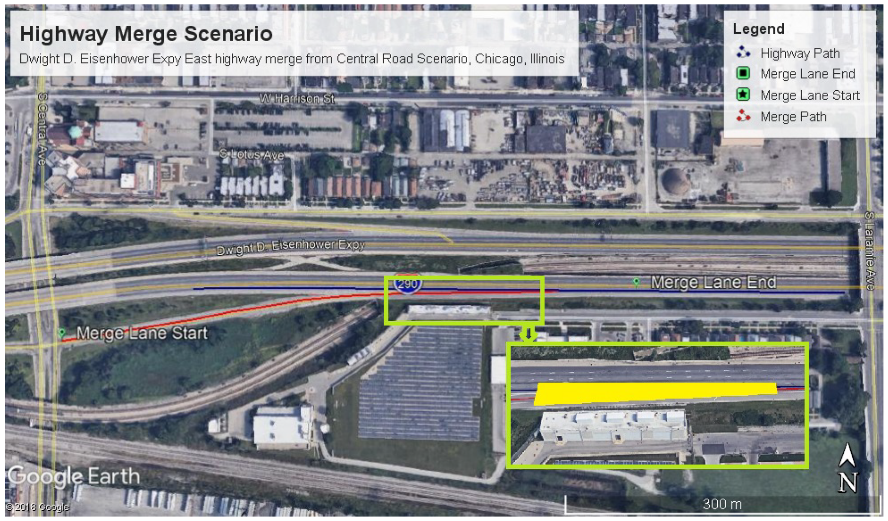
3.4. Highway Merge Case of Dwight D. Eisenhower Expressway (I-290)
Many of the tapered highway merge designs have close to no surplus road in order for the local lane vehicle to implement a smooth merge. As an example, the merge from Central Avenue to the Dwight D. Eisenhower Expressway, commonly referred to as I-290, presents a similar challenge. A Google® top view image [30] of the expressway starting near Central Avenue created from the desktop application Google Earth PRO® is shown in Figure 4.
The picture shows the local merge lane highlighted in the red path, starting at a traffic sign, and continuing to the Eisenhower Expressway. The highway path is marked by a blue line on the expressway to show the rightmost highway lane. Using the scale (shown at the bottom of the picture), the complete merge path measured is approximately 800 m in length. The top view clearly shows the merge area between the highway lane and the merge lane as marked by the yellow rectangle in the inset picture. It is a short path of about 90 m, narrowing towards the east. The short merge path presents a considerable challenge during the merge process, given the speed of the expressway, as explained in the next subsection.
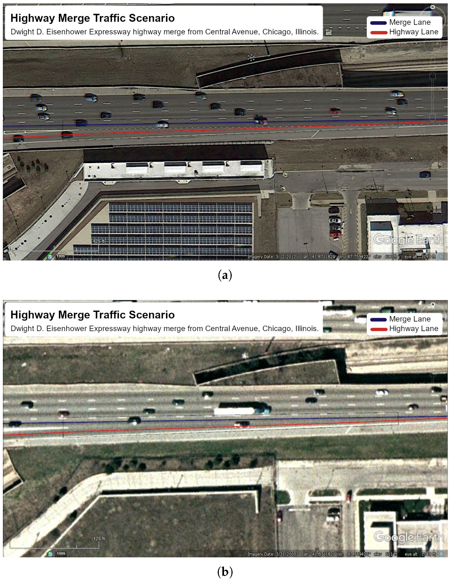
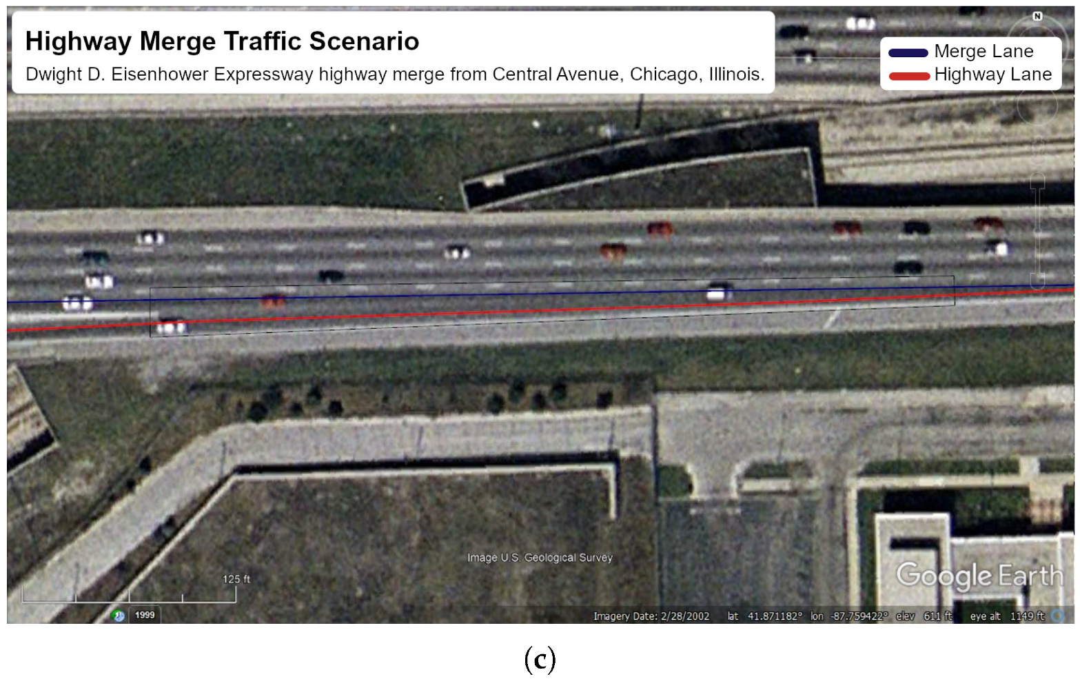
3.4.1. Traffic Conditions of the Highway Merge Lane
This section discusses a couple of Google® satellite images [30] taken from its historical image sets. Observe three cars in the highway lane, and two cars in the local merge lane in the first image (Figure 5a). The highway merge process has to be very quick and efficient, with the desired speed of 55 mph on the expressway.
In the second image (Figure 5b), a vehicle is in the middle of the merge process, with two vehicles trailing it on the highway. This image shows how short the distance would be for the merging vehicle to perform the highway merge from the merge lane. In the final image (Figure 5c), a merging vehicle seems to have completed the merge process with two cars trailing it on the highway.
The speed limit in the local lanes is usually 25 mph (appx. 11 m/s), and the expressway lane speed is 55 mph (appx. 25 m/s). A transition has to be made between these two speeds, and a simple step reference profile is used to represent this transition at approximately 400 m towards east starting at the central traffic junction near the start of the local lane.
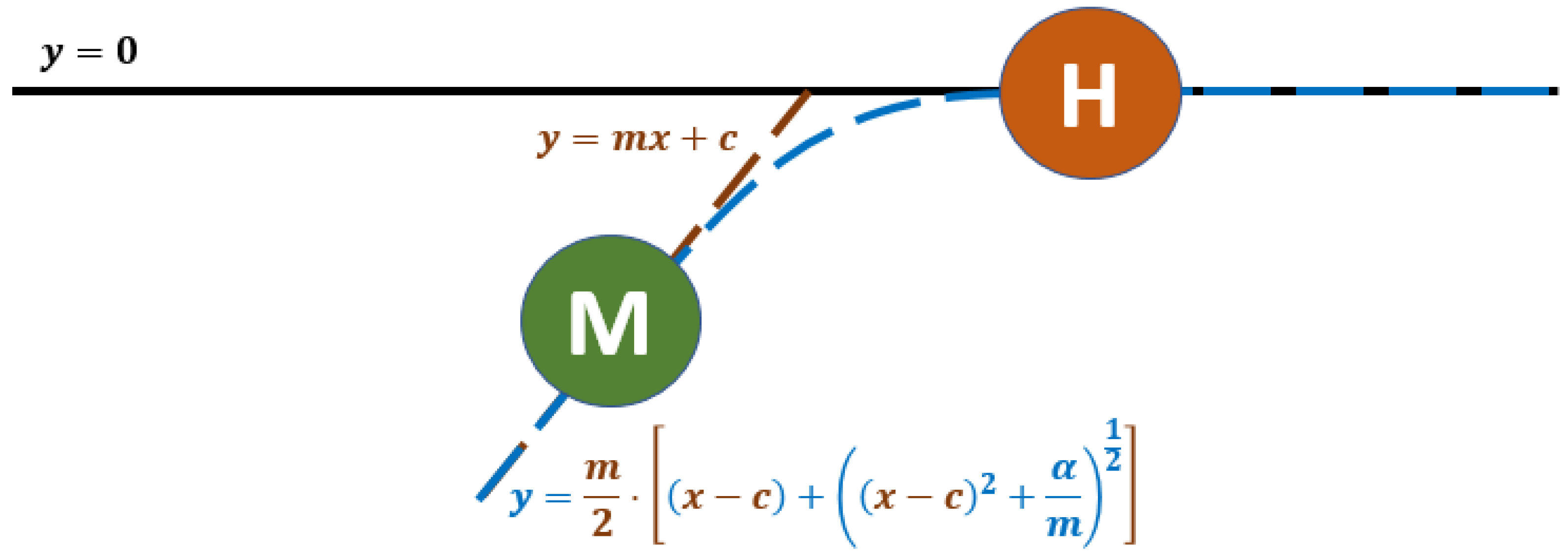
3.4.2. Reference Trajectory Profile
Figure 6 shows the profiles of the highway and the local merge lane.
The equation in Figure 6 describes the equation of the reference trajectory profile [31], where variables x and y are the x-coordinates and y-coordinates of the merge lane, m is the slope of the merge lane, c is the x-intercept of the merge lane, and is the smoothing factor to smooth out the profile.
The parameters are selected such that they match any given profile of the merge lane. The highway lane for the merge process is approximated by the x-axis () shown by a blue line in Figure 4. The local merge lane starts at an over-bridge signal and joins the highway lane at approximately 300 m after that traffic signal. The parameters for the local lane reference trajectory are shown in Table 1. For simulation purposes, the reference for the highway lane was kept at the origin.
4. Nonlinear MPC Cooperative Model Formulation
Using the reference trajectory as defined above and with the nonlinear kinematic bicycle model for a single vehicle, the formulation of the nonlinear merge lane tracking was simulated first, considering the following cost functions and constraints:
- Minimizing the state error between the desired and actual;
- Minimizing the control effort for both lateral and longitudinal control inputs;
- Minimizing control deviations in order to obtain controls that implement a smooth highway merge.
Then, a cooperation MPC optimization formulation was added that minimizes the deviations of states and inputs along with two more considerations as described below:
- Penalizing the proximity between the two vehicles;
- Taking in to account driver comfort.
4.1. Objective Cost
The objective cost can be divided into three different cost functions as follows: tracking, safety, and comfort costs.
4.1.1. Tracking Cost
The tracking cost is minimized to include the squared error between the desired states () and their respective actual states (z), as described in Equation (1). are weights to state errors, is the initial time, T is the sampling time, and horizon H is parameterized into k steps. This part of the cost function evaluates the deviations of displacement of merge and highway vehicles from their respective lanes, the merge vehicle yaw deviation from the reference yaw, and the velocity deviations of both vehicles with reference to the posted speed limits.
4.1.2. Safety Cost
A relative distance parameter is introduced in the proximity or safety cost. Sigmoid functions are constructed, which depends on the relative gap between the merge and highway vehicles, to smooth the proximity cost function, as shown in Equation (3).
where is defined as
in which the variable is the sigmoid tuning parameter for the distance cost.
4.1.3. Comfort Cost
The comfort cost includes the variation of the acceleration control inputs and their derivatives referred to generally as jerks. The steering rate or steering jerk should be limited to minimize the large deviations or oscillations in the system. The acceleration and deceleration rates, which are commonly called acceleration jerks, are regulated rather than tracked in the cost function and minimized to achieve smooth control.
Combining all the three cost forms the objective cost of the cooperative merge, as shown below:
4.2. Constraints
The state constraints are applied only on the velocity states for both vehicles involved in the merge process. As such, the velocities are constrained to the lane speed limits, as shown by Equations (7) and (8).
The inputs are acceleration for both merge and highway vehicles. The steering input refers to the merging vehicle only. The maximum and minimum values of inputs are bound by the acceleration values. As before, the throttle and braking are combined as one constraint to limit both vehicle acceleration and deceleration. All input constraints are given from Equations (9) to (11).
As mentioned in Section 3.3, at time t, the Nonlinear Model Predictive Controller (NMPC) solves Equations (2)–(5) using the kinematic model described in Equation (1) subject to constraints (Equations (7)–(11)) to return the inputs for the complete horizon. The first control input is then applied to the system and is repeated in receding order.
5. Results and Discussion
The ACADO–MATLAB toolkit was used in connection with the MATLAB® simulation environment. The ACADO code for vehicle kinematic simulations was first written and tested to verify the kinematic formulation.
Using parameters for the reference curve and respecting the speed limits of the local and highway lanes, the simulation was performed for the most common highway merge scenarios. Each scenario is discussed in detail in the following subsections. The weights used in the Lagrangian least square formulations of the objective function for a cooperative merge in each scenario are presented in Table 2. As one can observe, the tuning was performed in such a way that the cost associated with y-displacement, velocity states, and safety are given more importance. The controls and control rates are also given due importance, such that the variations of the controls are smooth and give a much better ride to the driver and its passengers, and jerks are regulated as much as possible.
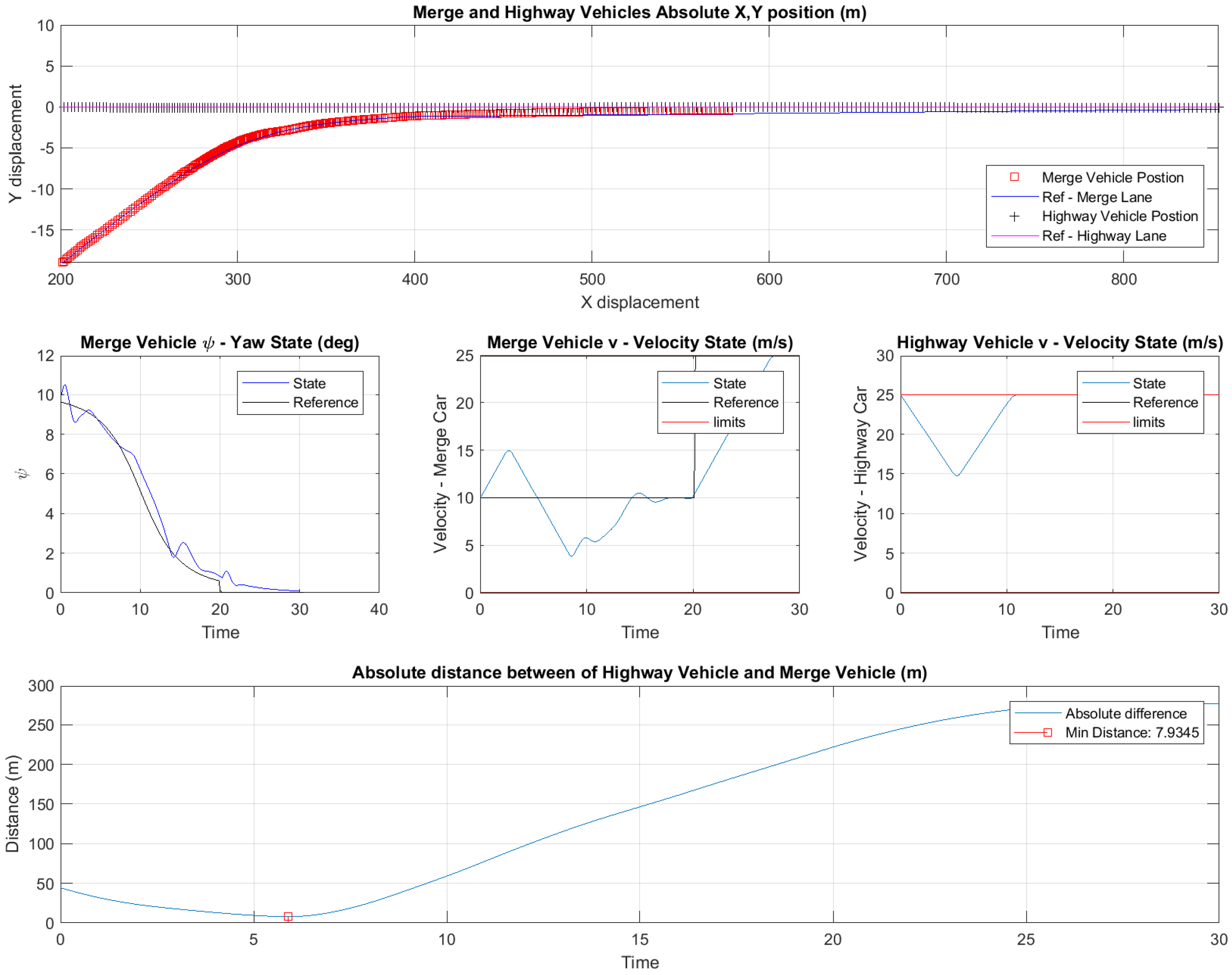
5.1. Scenario 1: Regular Traffic—Vehicles Speeds Close to Desired
Each scenario presents the most common situations that can be encountered during a highway merge. In the first demonstration, it is assumed that during normal traffic conditions, the merge and highway vehicles are close to the speed limits of each lane, respectively. This test was designed to simulate the safety of vehicles as the distance between them is reduced. It was expected that the optimization would emphasize the proximity and trajectory while ignoring other cost functions. The initial conditions for this scenario are shown in Table 3.
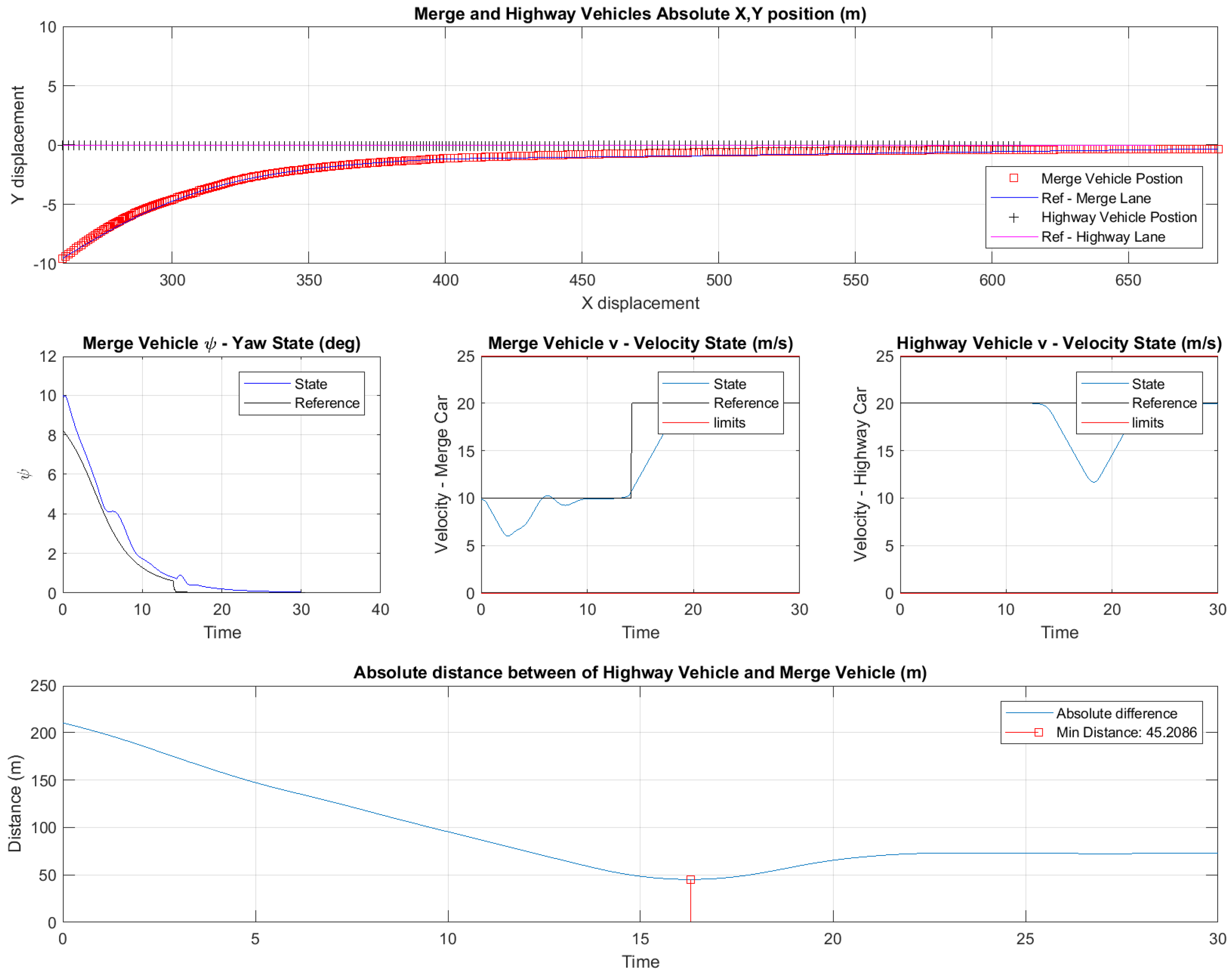
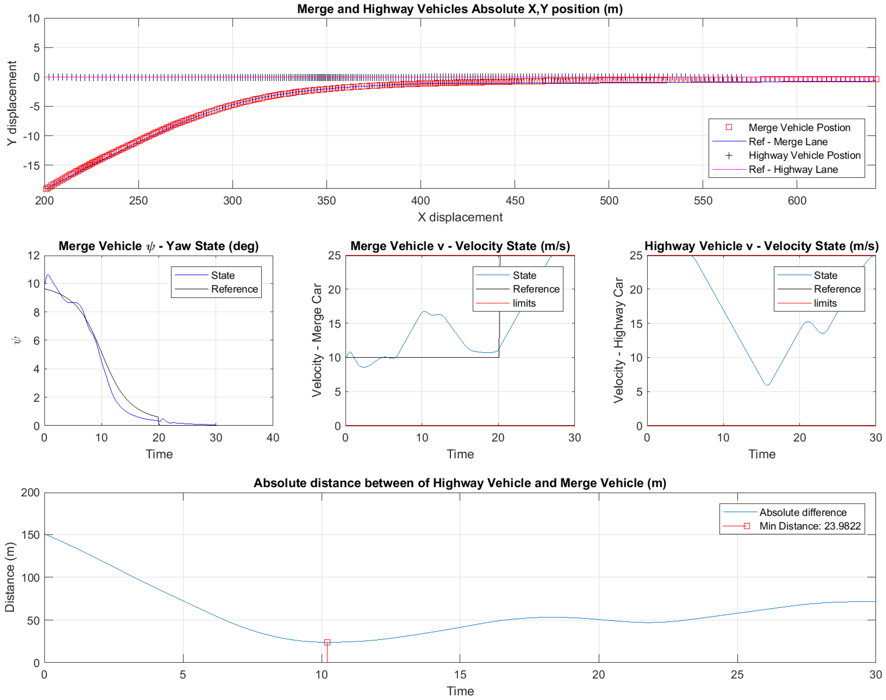
The state trajectories of the merge and highway vehicles during the optimization are presented in Figure 7.
It is observed that the merge vehicle and the highway vehicle are able to track the reference trajectories very closely with the yaw of the merge vehicle close enough to the reference profile. Since, the safety of the vehicles was important, the velocities did not closely adhere to the respective lane speeds. It can be observed that initially the merge vehicle speed increased while the highway vehicle speed reduced, but later, the highway vehicle speed increased and the merge vehicle’s brakes were applied in order for the highway vehicle to take the lead in the merging process. In the last plot, the longitudinal separation between the highway vehicle and merge vehicle is presented. The plot also shows the closest the vehicles come to each other while performing the merge.
As the merge vehicle enters the 400 m mark, which defines the start of highway, the merge vehicle smoothly follows the speed limit, and in a smooth transition happens to adhere to the speed limits of the highway lane. Meanwhile, the highway vehicle continues with a speed of 25 m/s. The minimum gap during the merge process between the two vehicles, in this case, is m.
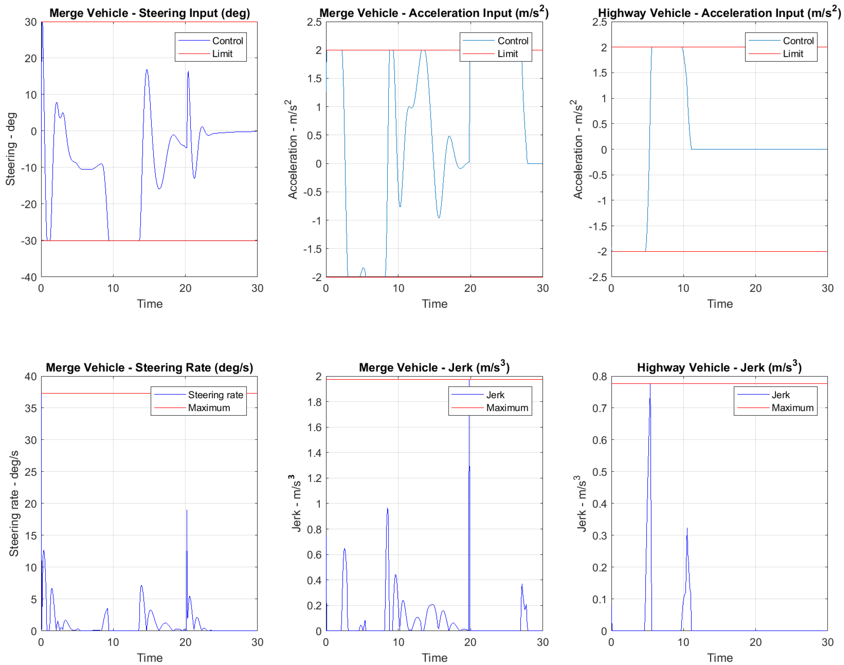
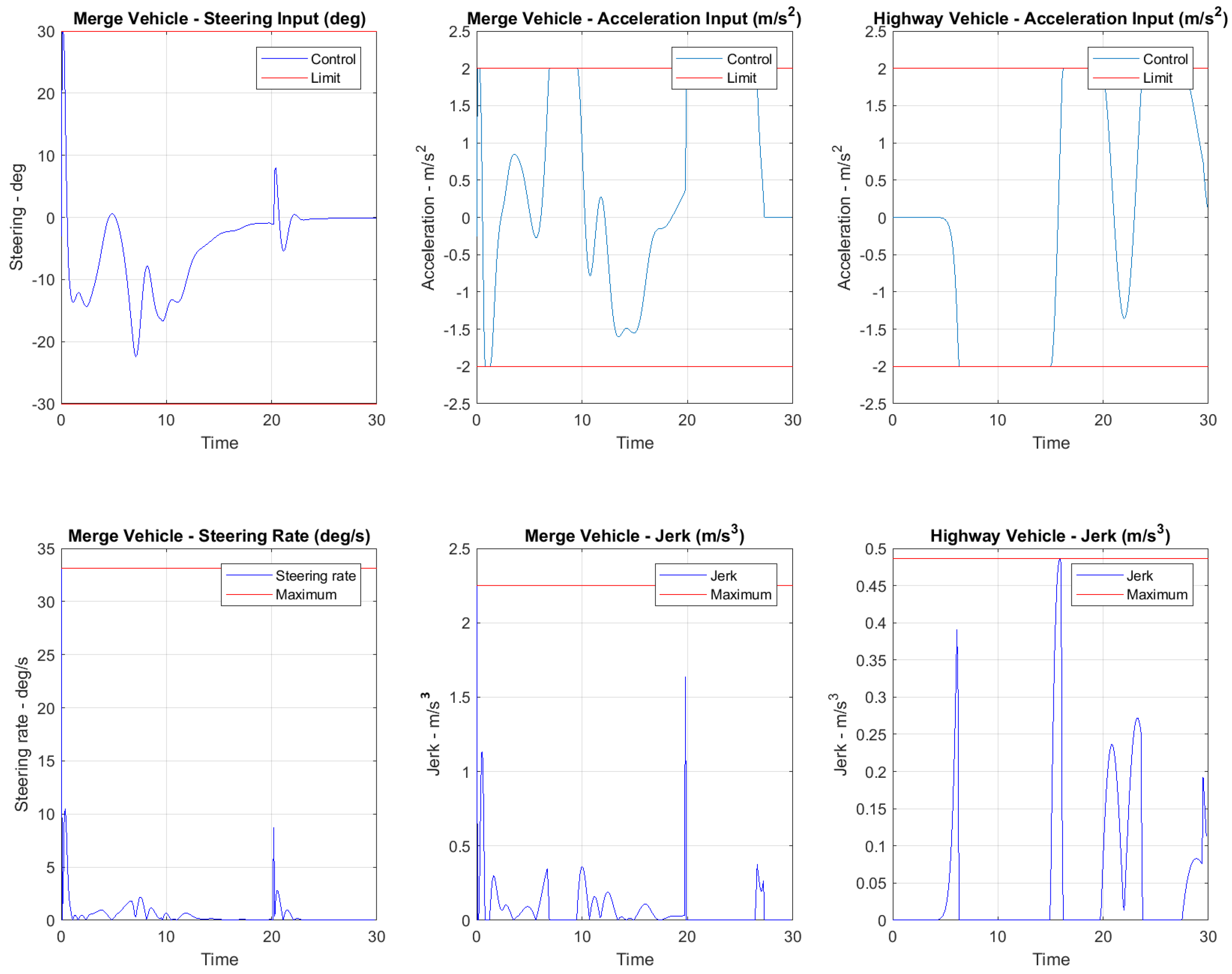
The controls to the merge vehicle and the highway vehicles are shown in Figure 8, which shows that the steering and accelerations are within the limits defined by the constraints of the optimization. The plot also includes the jerks experienced by both vehicles. The objective was to have it close to zero as regulated in the cost function. The absolute maximum jerk rates are shown by the red limit line and remain within the comfort limits of driving.
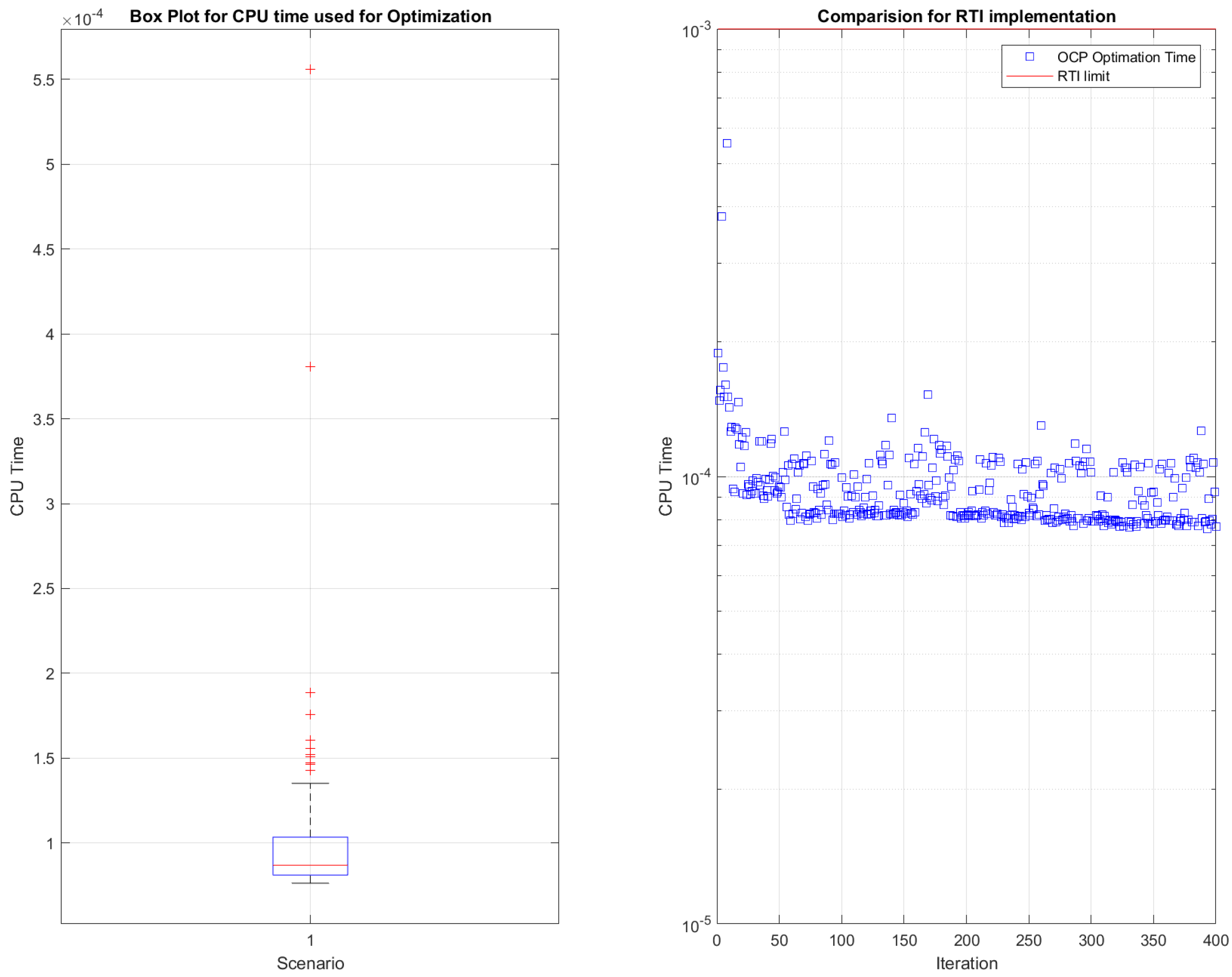
The simulation was performed on a desktop personal computer with an Intel-3 processor and 8 Gb of memory using MATLAB® 2017a. Figure 9 shows the box plot of the CPU computation time for each optimization step; on the right, it shows the logarithmic plot of the CPU computation time with respect to the Real-Time Implementation (RTI) limit set at one millisecond. As observed, most of the computation of the control steps is a 10th less than the RTI limit which shows that the algorithm can be implemented in real time.
5.2. Scenario 2: Scenario When Merge Vehicle Enters the Highway Lane First
In some cases, even though the merge car is slower, because it is following the merge lane speed limit, it can enter the highway lane first as it is in close proximity to it. This scenario tests such a case. When it happens, the fast moving highway vehicle has to respect the safety constraint and slow down and allow the merge vehicle to gain its speed while still respecting the traffic speed limits. The initial conditions for this scenario are shown in the Table 4
The state trajectories of the merge and highway vehicles during optimization are presented in Figure 10 for 40 s to show the merge process.
The velocity of the merge vehicle is close enough to the lane speeds, but as the merge vehicle approaches the highway path, it receives cautions and reduces its speed, and when it enters the highway, it transitions to adhere to the strict speed limits of the highway lane. Meanwhile, the highway vehicle speed is reduced in such a way that the safety criterion is maintained, and as soon as the leading merge vehicle increases its speed, it follows closely to continue its route at the desired speed. It can be observed that the vehicle longitudinal distance maintains the safety limit set by the criterion very well.
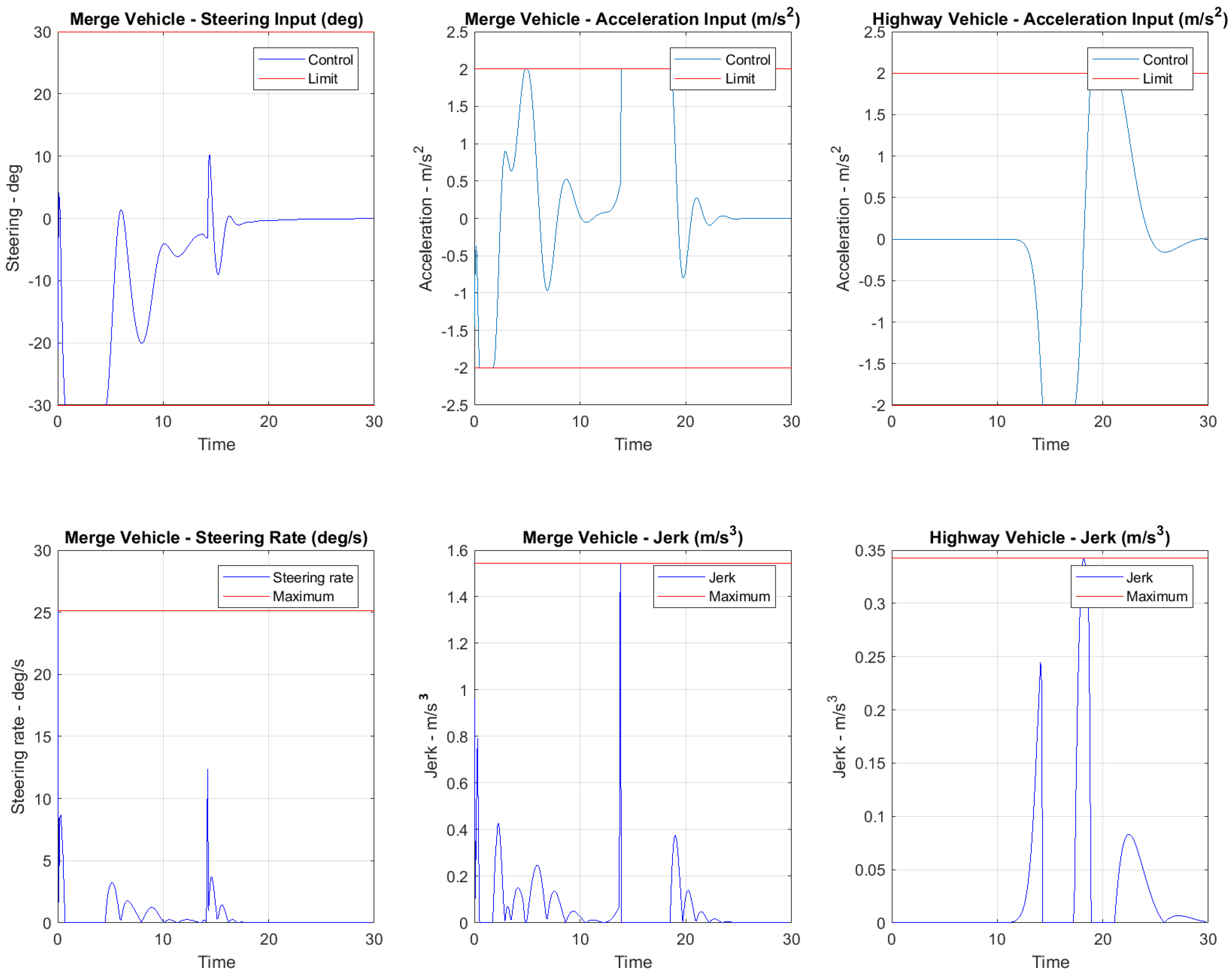
During this scenario, the controls applied and jerks experienced by the merge vehicle and the highway vehicles are shown in Figure 11. Again, they are both within the satisfactory limits.
5.3. Scenario 3: Close Call, Control Speeds Up/Slows Down Vehicles to Complete the Merge
This scenario tests the optimization scheme when the distance between the vehicles is very close. It is expected that in such a scenario, if one of the vehicles gives in, the other vehicle will takes the lead respecting safety and tracking the objectives. To generate such a case, the initial conditions of the simulations were modified, as shown in the Table 5.
The state trajectories of the merge and highway vehicles during optimization are presented in Figure 12 for 40 s to show the merge process. It can be observed that the merge vehicle speeds up and deviates from the reference speed profile, while the highway vehicle slows down and allows the merge vehicle to lead the merge process, which can also be observed in some cases of human driving. During this scenario, the controls applied and jerks experienced by the merge vehicle and the highway vehicles are shown in Figure 13.
6. Conclusions
A cooperative Nonlinear Model Predictive Control (NMPC)-based optimization method is developed for a highway merge maneuver, while respecting the relevant constraints. A cooperative control is a form of autonomous merge in which a merge is implemented between a ’merge’ vehicle in the local lane and a ’highway’ vehicle close by in the highway lane, with some communication between the two. The optimization considered tracking, safety, and driving comfort subject to the model dynamics of the process. The optimization used kinematic vehicle models which have a lower computational load compared to dynamic vehicle models for state predictions. The cooperative strategy is solved using direct simultaneous multishooting techniques. Using a highway merge profile on the Dwight Eisenhower Expressway (I-290) in Chicago, Illinois, this paper presents simulation results for various highway merge scenarios. It was assumed that the highway merge vehicle was part of the merge process.
Author Contributions
S.A.H. reviewed the literature, narrowed the research, formulated the problem, developed methodology, wrote the software, validated the results and did the analysis. B.S.J. was equally involved in the conceptualization of the problem, literature review, and initial investigation of the problem statement. S.C. supervised the overall research, reviewed the conceptualization, project administration, and funding acquisition. All the authors contributed equally towards the review process of this paper. All authors have read and agreed to the published version of the manuscript.
Funding
This research was funded by the University of Illinois at Chicago, College of Engineering and partially funded by Servotech Inc.
Acknowledgments
The authors would like to acknowledge the University of Illinois at Chicago to providing the resources for completing this research.
Conflicts of Interest
The authors declare no conflict of interest.
References
- Litman, T. Autonomous Vehicle Implementation Predictions; Victoria Transport Policy Institute: Victoria, BC, Canada, 2017. [Google Scholar]
- Waldrop, M.M. No drivers required. Nature 2015, 518, 20. [Google Scholar] [CrossRef] [PubMed]
- Walker, J. The Self-Driving Car Timeline–Predictions from the Top 11 Global Automakers. Abrufdatum. 2018. Available online: https://www.techemergence.com/self-driving-car-timeline-themselves-top-11-automakers/ (accessed on 1 August 2018).
- Federal Automated Vehicles Policy. Accelerating the Next Revolution in Roadway Safety; NHTSA, US Dept. Transportation: Washington, DC, USA, 2016.
- National Highway Traffic Safety Administration. Automated Driving Systems 2.0: A Vision for Safety; National Highway Traffic Safety Administration: Washington, DC, USA, 2017.
- Shahian Jahromi, B.; Tulabandhula, T.; Cetin, S. Real-Time Hybrid Multi-Sensor Fusion Framework for Perception in Autonomous Vehicles. Sensors 2019, 19, 4357. [Google Scholar] [CrossRef] [PubMed] [Green Version]
- Shahian-Jahromi, B.; Hussain, S.A.; Karakas, B.; Cetin, S. Control of autonomous ground vehicles: A brief technical review. IOP Conf. Ser. Mater. Sci. Eng. 2017, 224, 012029. [Google Scholar] [CrossRef]
- Meinel, H.H. Commercial Applications of Millimeterwaves History, Present Status, and Future Trends. IEEE Trans. Microw. Theory Tech. 1995, 43, 1639–1653. [Google Scholar] [CrossRef]
- Rajamani, R.; Shladover, S. An experimental comparative study of autonomous and co-operative vehicle-follower control systems. Transp. Res. Part C Emerg. Technol. 2001, 9, 15–31. [Google Scholar] [CrossRef]
- Rajamani, R.; Tan, H.S.; Law, B.K.; Zhang, W.B. Demonstration of integrated longitudinal and lateral control for the operation of automated vehicles in platoons. IEEE Trans. Control. Syst. Technol. 2000, 8, 695–708. [Google Scholar] [CrossRef]
- Hernandez-Jayo, U.; Mammu, A.S.K.; De-la Iglesia, I. Reliable communication in cooperative ad hoc networks. In Contemporary Issues in Wireless Communications; IntechOpen: London, UK, 2014; Available online: https://www.intechopen.com/books/contemporary-issues-in-wireless-communications/reliable-communication-in-cooperative-ad-hoc-networks (accessed on 25 March 2020). [CrossRef] [Green Version]
- Kesting, A.; Treiber, M.; Helbing, D. General Lane-Changing Model MOBIL for Car-Following Models. Transp. Res. Rec. J. Transp. Res. Board 2007, 1999, 86–94. [Google Scholar] [CrossRef] [Green Version]
- Chee, W.; Tomizuka, M. Vehicle Lane Change Maneuver in Automated Highway Systems; UC Berkeley: Berkeley, CA, USA, 1994. [Google Scholar]
- Kim, K.; Cho, D.i.; Medanic, J.V. Lane assignment using a genetic algorithm in the automated highway systems. In Proceedings of the 2005 IEEE Intelligent Transportation Systems, Vienna, Austria, 16 September 2005; pp. 540–545. [Google Scholar]
- Chee, W. Unified Lateral Control System for Intelligent Vehicles. SAE Trans. 2000, 109, 531–539. [Google Scholar]
- Hatipoglu, C.; Ozguner, U.; Redmill, K.A. Automated lane change controller design. IEEE Trans. Intell. Transp. Syst. 2003, 4, 13–22. [Google Scholar] [CrossRef]
- Gidlewski, M.; Zardecki, D. Automatic Control of Vehicle steering system during lane change. In Proceedings of the 24th International Technical Conference on the Enhanced Safety of Vehicles (ESV), National Highway Traffic Safety Administration, Gothenburg, Sweden, 8 June 2015; p. 15-0106. [Google Scholar]
- Snider, J.M. Automatic Steering Methods for Autonomous Automobile Path Tracking; Tech. Rep. CMU-RITR-09-08; Robotics Institute: Pittsburgh, PA, USA, 2009. [Google Scholar]
- Hussain, S.A.; Shahian-Jahromi, B.; Karakas, B.; Cetin, S. Highway lane merge for autonomous vehicles without an acceleration area using optimal Model Predictive Control. World J. Res. Rev. 2018, 6, 27–32. [Google Scholar] [CrossRef]
- Rios-Torres, J.; Malikopoulos, A.A. A Survey on the Coordination of Connected and Automated Vehicles at Intersections and Merging at Highway On-Ramps. IEEE Trans. Intell. Transp. Syst. 2016, 1066–1077. [Google Scholar] [CrossRef]
- Kachroo, P.; Li, Z. Vehicle merging control design for an automated highway system. In Proceedings of the IEEE Conference on Intelligent Transportation System, ITSC’97, Boston, MA, USA, 12 November 1997; pp. 224–229. [Google Scholar]
- Cao, W.; Mukai, M.; Kawabe, T.; Nishira, H.; Fujiki, N. Gap Selection and Path Generation during Merging Maneuver of Automobile Using Real-Time Optimization. SICE J. Control. Meas. Syst. Integr. 2014, 7, 227–236. [Google Scholar] [CrossRef]
- Cao, W.; Mukai, M.; Kawabe, T.; Nishira, H.; Fujiki, N. Cooperative vehicle path generation during merging using model predictive control with real-time optimization. Control Eng. Pract. 2015, 34, 98–105. [Google Scholar] [CrossRef]
- Rajamani, R. Vehicle Dynamics and Control; Mechanical Engineering Series; Springer: Boston, MA, USA, 2012; p. 498. [Google Scholar] [CrossRef]
- Bulirsch, R.; Vögel, M.; von Stryk, O.; Chucholowski, C.; Wolter, T.M. An optimal control approach to real time vehicle guidance. In Mathematics—Key Technology for the Future; Springer: Berlin/Heidelberg, Germany, 2003; pp. 84–102. [Google Scholar] [CrossRef]
- Mokhiamar, O.; Abe, M. Simultaneous Optimal Distribution of Lateral and Longitudinal Tire Forces for the Model Following Control. J. Dyn. Syst. Meas. Control 2004, 126, 753. [Google Scholar] [CrossRef]
- Zeping, F.; Jianmin, D. Optimal lane change motion of intelligent vehicles based on extended adaptive pseudo-spectral method under uncertain vehicle mass. Adv. Mech. Eng. 2017, 9, 1–15. [Google Scholar] [CrossRef] [Green Version]
- Diehl, M.; Bock, H.G.; Schlo, J.P.; Findeisen, R.; Nagy, Z.; Allgo, F.; Schlöder, J.P.; Findeisen, R.; Nagy, Z.; Allgöwer, F. Real-time optimization and nonlinear model predictive control of processes governed by differential-algebraic equations. J. Process Control 2002, 12, 577–585. [Google Scholar] [CrossRef]
- Houska, B.; Ferreau, H.J.; Vukov, M.; Quirynen, R. ACADO Toolkit User’s Manual. Available online: http://www.acadotoolkit.org (accessed on 12 August 2018).
- Google Earth Pro. Dwight D. Eisenhower Expressway between Central Ave and Laramie Ave. Google Earth Pro, 2018. Available online: https://www.google.com/earth/ (accessed on 1 August 2018).
- Cao, W.; Mukai, M.; Kawabe, T. Two-dimensional merging path generation using model predictive control. Artif. Life Robot. 2013, 17, 350–356. [Google Scholar] [CrossRef]
Figure 1.
Typical cooperative lane merge maneuver.

Figure 2.
Types of highway merge ramps.

Figure 3.
Highway merge using two vehicles.

Figure 4.
Top view of Eisenhower Expressway starting near Central Avenue, Chicago, IL, USA.

Figure 5.
Traffic on Dwight D. Eisenhower Expressway for a highway merge from Central Avenue, (Lat. and Lon. ) [30]. (a) Traffic image date: 12 March 2012; (b) image date: 31 March 2005; (c) image date: 28 February 2005.
Figure 5.
Traffic on Dwight D. Eisenhower Expressway for a highway merge from Central Avenue, (Lat. and Lon. ) [30]. (a) Traffic image date: 12 March 2012; (b) image date: 31 March 2005; (c) image date: 28 February 2005.


Figure 6.
Equations describing the highway lane and merge lane.

Figure 7.
State cooperative merge scheme—Scenario 1.

Figure 8.
Optimized control—Scenario 1.

Figure 9.
CPU optimization time—Scenario 1.

Figure 10.
State cooperative merge scheme—Scenario 2.

Figure 11.
Optimized control—Scenario 2.

Figure 12.
State cooperative merge scheme—Scenario 3.

Figure 13.
Optimized control—Scenario 3.


Table 1.
Local lane trajectory parameters.
| Reference Trajectory Parameters of the Local Lane | ||
|---|---|---|
| Slope (m) | Smoothing () | X-Intercept (c) |
| 0.18 | 500 | 300 |
Table 2.
Tuning parameters for cooperative merge—Scenario 1.
| Weights for Objective Cost Functions | |||||
|---|---|---|---|---|---|
| Tracking–Weights | Distance–Weight | ||||
| functiondist | |||||
| 1 | 1 | 1 | 1 | 8 | |
| Comfort–Weights | |||||
| 1 | 2 | 5 | 5 | 5 | 5 |
Table 3.
Initial conditions for Scenario 1.
| Initial Conditions for Scenario 1: Regular Traffic | |||||
|---|---|---|---|---|---|
| 200 m | −18 m | 10 | 5 m/s | 100 m | 25 m/s |
Table 4.
Initial conditions for Scenario 2.
| Initial Conditions for Scenario 2: Merge Vehicle First | |||||
|---|---|---|---|---|---|
| 260 m | −18 m | 10 | 10 m/s | 50 m | 20 m/s |
Table 5.
Initial conditions for Scenario 3.
| Initial Conditions for Scenario 3: Close Call | |||||
|---|---|---|---|---|---|
| 200 m | −18 m | 10 | 10 m/s | 100 m | 25 m/s |
© 2020 by the authors. Licensee MDPI, Basel, Switzerland. This article is an open access article distributed under the terms and conditions of the Creative Commons Attribution (CC BY) license (http://creativecommons.org/licenses/by/4.0/).
Share and Cite
MDPI and ACS Style
Hussain, S.A.; Shahian Jahromi, B.; Cetin, S. Cooperative Highway Lane Merge of Connected Vehicles Using Nonlinear Model Predictive Optimal Controller. Vehicles 2020, 2, 249-266. https://0-doi-org.brum.beds.ac.uk/10.3390/vehicles2020014
AMA Style
Hussain SA, Shahian Jahromi B, Cetin S. Cooperative Highway Lane Merge of Connected Vehicles Using Nonlinear Model Predictive Optimal Controller. Vehicles. 2020; 2(2):249-266. https://0-doi-org.brum.beds.ac.uk/10.3390/vehicles2020014
Chicago/Turabian StyleHussain, Syed A., Babak Shahian Jahromi, and Sabri Cetin. 2020. "Cooperative Highway Lane Merge of Connected Vehicles Using Nonlinear Model Predictive Optimal Controller" Vehicles 2, no. 2: 249-266. https://0-doi-org.brum.beds.ac.uk/10.3390/vehicles2020014