Adaptive Neural Motion Control of a Quadrotor UAV


1
División de Mecatrónica, Tecnológico de Estudios Superiores de Tianguistenco, Carretera Tenango—La Marquesa Km. 22, Santiago Tilapa, Tianguistenco, Mexico State C.P. 52650, Mexico
2
División de Ingeniería Eléctrica, Facultad de Ingeniería, Universidad Nacional Autónoma de México, Av. Universidad 3000, Cd. Universitaria, Delegación Coyoacán, Mexico City C.P. 04510, Mexico
3
Departamento de Energía, Universidad Autónoma Metropolitana, Unidad Azcapotzalco, Av. San Pablo No. 180, Col. Reynosa Tamaulipas, Mexico City C.P. 02200, Mexico
*
Author to whom correspondence should be addressed.
†
These authors contributed equally to this work.
Vehicles 2020, 2(3), 468-490; https://0-doi-org.brum.beds.ac.uk/10.3390/vehicles2030026
Submission received: 22 May 2020
/
Revised: 12 July 2020
/
Accepted: 16 July 2020
/
Published: 20 July 2020
(This article belongs to the Special Issue Autonomous Vehicle Control)
Abstract
:Unmanned Aerial Vehicles have generated considerable interest in different research fields. The motion control problem is among the most important issues to be solved since system dynamic stability depends on the robustness of the main controller against endogenous and exogenous disturbances. In spite of different controllers have been introduced in the literature for motion control of fixed and rotary wing vehicles, there are some challenges for improving controller features such as simplicity, robustness, efficiency, adaptability, and stability. This paper outlines a novel approach to deal with the induced effects of external disturbances affecting the flight of a quadrotor unmanned aerial vehicle. The aim of our study is to further extend the current knowledge of quadrotor motion control by using both adaptive and robust control strategies. A new adaptive neural trajectory tracking control strategy based on B-spline artificial neural networks and on-line disturbance estimation for a quadrotor is proposed. A linear extended state observer is used for estimating time-varying disturbances affecting the controlled nonlinear system dynamics. B-spline artificial neural networks are properly synthesized for on-line calculating control gains of an adaptive Proportional Integral Derivative (PID) scheme. Simulation results highlight the implementation of such a controller is able to reject disturbances meanwhile perform proper motion control by exploiting the robustness, disturbance rejection, adaptability, and self-learning capabilities.
1. Introduction
The interest in the study of unmanned aerial vehicles (UAV) has increased in the last years since these aerial machines are able to accomplish several sorts of tasks. Diverse configurations of these vehicles one may encounter in many different applications, e.g., surveillance, monitoring, inspection, mapping, or payload transportation [1]. The four-rotor helicopter is a rotary-wing unmanned aerial vehicle (RW-UAV) commonly named as quadrotor [2]. This has been the focus of various technological and scientific research works. This vehicle is an underactuated system, due to it counts with six degrees of freedom and only four independent control inputs; providing this platform the ability of vertical take off and landing (VTOL). This feature allows its safe operation in interiors, unlike other UAV’s such as the fixed wing (FW-UAV) type that need large and wide space extensions for take-off and landing [3].
During their operation, quadrotors are subject to endogenous and exogenous uncertainties, due to a highly changing medium as a consequence of variable wind speeds, fluctuations in the surrounding humidity and air resistance. Thus, a complex non-linear dynamic behaviour between relevant variables and uncertainty is observed. Taking this into consideration, and in order to perform tasks of trajectory tracking, slow and fast motion, hovering, stable flight and VTOL, the design of robust motion control schemes is necessary.
Different linear and nonlinear control strategies have been proposed in the literature for control of quadrotor helicopters. In [4], conventional proportional integral derivative controller (PID) and linear quadratic (LQ) controllers are developed for stabilization tasks for a quadrotor in presence of small perturbations. PID control algorithms have been also introduced in [5]. Here, results show that the proposed controller presents a good performance for flight in controlled environments and a trajectory tracking with relatively slow speed only. In spite of being unable to deal with large disturbances, classical controllers present a compact and functional structure which has allowed their successful implementation in commercial models [6].
In some works, diverse control strategies composed of conventional and nonlinear robust controllers are introduced to deal efficiently with external disturbances, model uncertainties, internal cross couplings and noisy sensor measurements. The introduced scheme in [7] consists of a backstepping based PID nonlinear controller to regulate the quadrotor rotational dynamics, the integral of tracking error is considered in the backstepping control design to minimize the steady-state error. The work developed in [8] deals with the regulation of position for the quadrotor through a robust PID control. Meanwhile, the attitude problem is solved by means of integral backstepping and terminal sliding mode controllers, providing robustness to the control loop against external disturbances.
Furthermore, diverse nonlinear robust controllers have been reported facing the disturbed helicopter dynamics, as is introduced in [9,10]. Here, the authors study the response of a quadrotor prototype for tracking trajectories by using backstepping and sliding mode strategies. In the first one, the backstepping control stage allows to compensate the rotational dynamics in presence of bounded perturbations. Nevertheless, sliding mode control introduces high frequencies to the system through the chattering phenomenon. Therefore, in the second proposal, the backstepping and sliding mode controllers are arranged to face the chattering phenomenon and the discontinuous action of control inputs, improving in this way the quadrotor tracking performance when unknown disturbances occur. Additionally, different schemes for enhancing sliding mode control performance have been also introduced in the literature. For example, in [11] a second order sliding mode controller is proposed for attenuating the switching problem without affecting the quadrotor flight performance. At the same time, in [12] unmatched perturbations and chattering problem are effectively solved by a block controller combined with the super twisting algorithm.
Besides, in [13] a nonlinear controller is introduced for controlling rotational dynamics and a model predictive controller (MPC) for performing tasks of trajectory tracking in the X and Y directions, in order to ensure a proper path following. In their study, authors consider external disturbances on the six degrees of freedom as well as parametric uncertainties. Meanwhile, in [6] robust compensators are proposed providing robustness to nominal PD control synthesis for attitude and position control in order to restrain the effects of uncertainties. Adaptive control has been proved to be powerful to handle parametric uncertainties and obtain asymptotic stability without using high-gain feedback or switching terms [14]. So, many authors have used adaptive controllers for solving the quadrotor control problem. Authors in [15] propose an adaptive control scheme with an intelligent observer based on artificial neural networks (ANN). Here, aerodynamic effects have been considered as disturbances. On the other hand, some modern nonlinear algorithms have been proposed as in [16] where a nonlinear internal model control (NLIMC) is introduced for controlling a quadrotor perturbed by wind gusts. The performance of the control is ensured by fixing a reference model of the tracking error. Meanwhile, in [17] a framework of Active Disturbance Rejection Control (ADRC) and Embedded Model Control (EMC) is proposed for robust attitude control of a four-rotor helicopter, where an state predictor, a control law, and a model-based reference generator are designed.
One of the main problems of the flight control systems is due to the combination of nonlinear dynamics, modelling uncertainties and parameter variation in characterizing an aircraft and its operating environment [18]. One fact that should be pointed out is that many uncertainties in control systems are unmeasurable; thus, the disturbance estimation technique represents a very good alternative to actively suppress time-varying disturbances [19,20]. Effectiveness and robustness of the ADRC has been proved for a wide range of engineering applications which involve different single input-output (SISO) and and multiple input - output (MIMO) systems (e.g., power converters [21], electric motor drives [22], mechanical systems [23], unmanned aerial vehicles [24], among others).
Some interesting ADRC based control schemes for the robust motion control of the quadrotor flight, have been reported. The proposed scheme in [25], implements a linear active disturbance rejection control (LADRC). Here, disturbances are estimated by a Linear Extended State Observer (LESO), and rejected by a PD controller; showing an acceptable control performance in overshoot, rise time and settle time. However, reported results consider weak disturbances only. On the other hand, authors in [26] propose a linear active disturbance rejection sliding mode control for addressing the system uncertainties and external disturbances, which are estimated by a LESO and afterwards, actively rejected through a sliding mode controller. In that study, slightly disturbed components are injected for altitude and attitude displacements in order to show the proposed controller performance. Meanwhile, even though ADRC control is able to reject the total disturbance, authors in [27] put all the available process information as an input in the control scheme for improving the disturbance estimation. On the other hand, in [28] satisfactory results are achieved to stabilize the system with a nonlinear modified version of the ADRC, where an extended state observer (ESO) is proposed for state estimation in order to deal with input delays and filter noisy output measurements of the variables of interest. Recently, the design and develop of modified and enhanced versions of the central ideas of the ADRC has been reported, as in [29]. Here, researchers propose a robust integral of sign of error (RISE) scheme and a disturbance compensation for the tracking trajectory of a quadrotor UAV. In that work, velocity measurements are unnecessary but the use of a third order ESO is required to achieve a high tracking performance.
In this work a novel robust adaptive neural motion control scheme for quadrotor vehicles is proposed. The presented control design method is based on synthesis of B-spline artificial neural networks (BsNN) and on-line estimation of dynamic disturbances, where an linear extended state observer is implemented to improve the robust control capability to actively suppress significant disturbances affecting the underactuated nonlinear system dynamics.
Efficiency and robustness of the controlled nonlinear dynamic system are significantly improved, since B-spline neural networks have capabilities for efficiently control physical systems by updating their response on-line, considering a simple structure and a small number of basic mathematical operations. Besides, the estimation of lumped disturbances allows to actively compensate it on-line by including in the nominal adaptive controller. In contrast with other controllers proposed in literature, in our scheme it is no necessary a full knowledge of the mathematical model and there is neither high frequency nor high gain behaviour of the control inputs due to the suitably selection of the PID-like controller gains by the B-spline neural networks.
Simulation results are included to verify that the novel control scheme represents a very good alternative to efficiently perform desired motion tracking for quadrotor helicopters. Moreover, simulations results yield that our motion control scheme can efficiently adapt to diverse uncertain operating scenarios even in presence of exogenous disturbances.
2. Dynamic Model
The quadrotor is an under-actuated and MIMO dynamic system with six degrees of freedom and only four control inputs. Moreover, its dynamic behaviour is governed by a set of strongly coupled nonlinear differential equations. A quadrotor is commonly designed to have a rigid body mechanical structure in order to obtain a simplified mathematical model, where two frames of reference are used to describe its dynamic behaviour [2,30]. The first inertial coordinate (global) frame reference with X, Y and Z axes is attached to the earth, and the second (local) one , with X’, Y’ and Z’ axes fixed to the centre of mass of the quadrotor as depicted in Figure 1. The suitably balanced mechanical structure has four rotors located symmetrically, which are used to generate the control force and torques represented as u, , and , respectively. Thus, force and torque controllers should be synthesized to perform on-line and off-line trajectory tracking for translation and rotation motion in the three-dimensional space planned for the quadrotor. The system motion is achieved by increasing or decreasing properly the speed of each rotor. The pair of rotors 1 and 3, spin counter-clockwise and the other in clockwise. Thus, pitching moment () is produced by rotors 1 and 3; rolling moment () is caused by the difference between forces produced by rotors 2 and 4; and yawing moment () is originated when angular velocities of lateral rotors are modified. Meanwhile, the control force u that allows lifting the body of the quadrotor, includes all the vertical forces produced by each rotor.
The relation between rotor forces () and control inputs is given by [2]
where l is the distance from the motors to the centre of mass and stands for the torque induced by each electric motor . and are related to the geometry of the rotors blades by means of the coefficients of thrust and drag. Hence, it is easy to see in Equation (1) that motion in different directions on the plane can be attained by regulating angular velocities of rotors in order to change the magnitude of the forces . Therefore, by suitably combining the rolling, pitching and yawing moments, a quadrotor can track different reference trajectories.
Exhaustive studies on the quadrotor mathematical model have been reported in the literature, where both numerical simulations an experimental tests have let to validate mathematical representations for describing the four-rotor helicopter dynamics. Since it is consider generally as a rigid body, representations as Newton-Euler, Euler-Lagrange and their derivations can be used to describe translational and rotational dynamics. Usually, a vector of generalized coordinates is used to represent the position and orientation of the body respect to the inertial reference frame as follows
where , and are the Euler angles describing the orientation of the system, and x, y and z are the position coordinates of the centre of mass (summarized as attitude vector and position vector , respectively) measured with respect to the inertial reference frame , as shown in Figure 1. Therefore, for purposes of control design, consider the following experimental validated quadrotor mathematical model [2,31,32], which is a Newton-Euler nonlinear simplified approximation around the hovering condition.
here, and represent the main force and torques acting on the quadrotor centre of mass expressed in the body frame. Meantime, is the velocity vector. The angular velocity vector is and is the inertia tensor, both regarding the body frame . The matrices and stand for skew-symmetric matrix of the vector [33] and the orthogonal rotation matrix (which allows to transform orientation between both reference frames, to [34,35]), respectively. Then, in order to express the equations regarding the inertial fixed frame, let and , where
The angular body velocities are related with rate of change of the Euler angles, which represent the quadrotor attitude in the inertial frame, under the next assumption
Thus, by using a standard kinematic transformation [33]
and assuming that in the zero vicinity the approximation , and is valid, the nonlinear dynamic model of the quadrotor can be resumed as follows
where m is the total quadrotor mass, and are the diagonal elements of the tensor of inertia expressed in the body frame, g the acceleration constant of gravity, is the gyroscopic effect resulting from the propeller rotation, with as the propeller moment of inertia and as the overall sum of rotors speed. On the other hand, and are the exogenous disturbances affecting the translational and rotational dynamics, respectively. Notice, that in spite of this model is a simplified version, rotational dynamics has numerous nonlinear couplings, which means that to solve the control problem it is not an easy task.
3. Motion Control Design
3.1. PID-Like Controller
The control approach is based on tracking errors given by the difference between real measured variables and desired reference trajectories,
for . Desired positions for regulation and trajectory tracking of the fully actuated motion are defined as and . Meantime, the virtual control stage computes the reference trajectories and by means of Equation (10), and, in this way, ensure the proper underactuated motion in X and Y directions. In this fashion, the virtual controllers to regulate underactuated dynamics are proposed as follows
with standing for an auxiliary controller introduced for controlling the vertical second order dynamics, . Hence, reference trajectories for and angles are given by
So, let introduce the following control inputs
where and are auxiliary design controllers. Furthermore, observe that the available model information is used in the control design as a compensation term. Therefore, the unperturbed position dynamics of the quadrotor is then governed by
with and . Thus, the auxiliary controllers are proposed with the following PID structure
where is the second derivative of the planned position reference. Then, by substituting Equations (13) and (11) in the equations set (7) the close-loop tracking error dynamics are given by
So, the closed-loop characteristic polynomial is
where the controller gains , and for , should be properly adjusted for ensuring closed-loop system stability. For instance, the coefficients of (15) can be selected matching the following Hurwitz characteristic polynomial
so that,
here , are the controller adjustment parameters for the properly tracking of the planned trajectory. In this work we compute on-line the controller parameters by using artificial neural networks.
3.2. Adaptive Control
Among the extensive list of automatic controllers, adaptive control has been proved to be powerful to handle parametric uncertainties and obtain asymptotic stability without using high-gain feedback or switching terms [14]. Thus, in this section the B-spline Artificial Neural Networks (BsNN) are used for the dynamic tuning of an adaptive control scheme using dynamic gains such as the introduced in (17). The synaptic weights are updated in every sample by using different learning index and inputs for each BsNN. This type of artificial neural networks are able to deal with the system nonlinearities and uncertainties, by means of the constant learning process of the physically system variables.
The scheme portrayed in Figure 2 shows the main architecture for each BsNN; a B-spline function is a polynomial mapping, which is compounded by a linear mix of the monovariable and multivariable basis functions, defined by its extremes. The associative networks, as the B-spline type, adjust iteratively their synaptic weights in order to reproduce a specific function. The updating process for associative networks is commonly performed by the use of least square algorithms, modifying in this way the index weight for each input of the basis function. The author in [36] proposes the BsNN output as follows
here y are the q- weight and the q- basis function input, respectively; and h is the number of synaptic weights. In this study we use the B-spline for calculating the gains of the whole controllers, with the output of each neural network defined as the control parameters for .
The learning process for an ANN is achieved through the error minimization, which is defined as difference between the actual output vector and the desired value [37]. In this work, the BsNN are training by using the following instantaneous learning rule [38]
here, is the learning rate and is the instantaneous output error. In this fashion, the training process is on-line performed continuously, meanwhile the weights values are updated by using the feedback variables. Its simply structure based on the basis functions constitutes only one internal layer, which becomes a powerful mechanism if the limits are properly bounded by choosing a correct knot vector and basis function shape [39].
In this work, different from our previous proposals [37], we use the BsNN for calculating the control gains in indirect way, it means by computing the control parameters introduced in (17). In this fashion, we try to constrain the BsNN whilst the Hurwitz stability condition keeps.
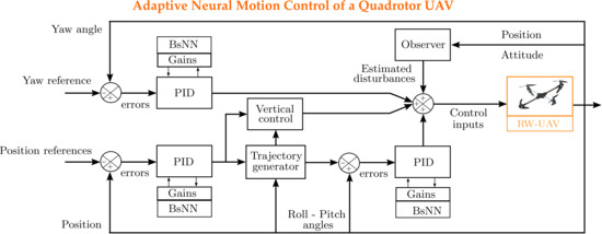
The summary of the control scheme is shown in the control diagram introduced in Figure 3. Here, the auxiliary vector is adopted to compact the representation of the proposal. Also, the position and attitude vectors are used to simplify the flux of the error information trough the circuit of control. Moreover we introduce the vector in order to simplify the representation.
Meanwhile, the trajectory generator in Equation (10) is summarized in TG block, which is continuously calculating the and in order to achieve a proper horizontal motion. On the other hand, PID blocks contains the controllers given in (13), where a proper mechanism to calculated the error integrals is included.
The control process is summarized as follows: firstly, the feedback values are compared with the planned references for the position and velocity variables and in order to calculate both the tracking errors and the auxiliary controllers. Later, the underactuation problem is solved by means of the virtual controllers and which are used within the TG block for updating the values of the angular references, and in this manner, ensuring close loop stability and the desire motion on the vertical and horizontal planes. Finally, and before the continuous process starts again, the actual control inputs are calculated and injected to the system as one force and three torques produced for the variations of angular velocity of their four rotors.
3.3. Extended State Observer Design
In order to provide the control scheme with a disturbance estimation mechanism, an extended state observer is introduced. Then, without loss of generality, we can represent the second order quadrotor dynamics (7) by the following state-space representation
where the function is the generalized disturbance [40] (involving external disturbance, unmodeled dynamics as well as parametric uncertainties). Therefore, assuming f is differentiable, with , equation set (20) can be written as an augmented state space
Then, by the implementation of a state observer it is possible to compute a good approximation of the disturbance, which is used as a compensation term added to the nominal control law. So, in spite of the original ADRC employs a non-linear observer, successfully results have been attained with the linear version introduced in [41], which deals efficiently with the observation problem. Then, in this work we use it as the main state observer, which is given as follows
with as the estimation error defined as for and are the observer gains, which are selected such that the third order characteristic polynomial is Hurwitz (stable).
A suitably selection of the observer gain vector guarantees the tracking of the real states. Therefore, the estimated states and the estimated generalized disturbance can be used in the controller design.
4. Numerical Experiments
Several numerical simulations are performed to asses the robustness of the proposed adaptive robust controller. Here, the control scheme should provide an acceptable level of attenuation of the exogenous disturbances for a flying quadrotor which is tracking a planned reference. The outline of the evaluation process is as follows: firstly, a nominal adaptive PID controller is evaluated for the unperturbed helicopter flight. Secondly, harmonic forces are injected to the system in order to visualize the response of the nominal controller. Finally, a scheme of disturbance estimation and compensation is attached to the nominal adaptive control law for improving their robustness capabilities.
The planned reference trajectories were selected in such a way a lemniscate path shape [42] is described on the horizontal X-Y plane. So, the individual dynamic references for x and y positions are given by the parametric equations and their derivatives depicted in Table 1.
A value of m is adopted for the distance to the origin to one of the lemniscate focus. Meanwhile, in order to asses the robustness and adaptability of the system to track a desire time-variable position , the mixture of step and variable profiles presented in Table 2 is used as the planned reference. On the other hand, a Bézier interpolation polynomial was implemented to obtain a smooth transient between initial and the desired yaw angle , which is given by
where: s, s, for ; s, s, for s; and , for s.
During indoors operations quadrotors are able to accomplish several kind of tasks without problems, but it is not the same for uncontrolled environments, where the surrounding medium is constantly changing, and different forces are induced as consequence of wind. So, one the main issues to be solved by the automatic control algorithms is the adaptation among different operational conditions. Thus, in our study some disturbing forces are used in order to simulate an probable outdoors uncontrolled medium.
4.1. Nominal Adaptive Control Performance
The performance of the introduced adaptive controller is portrayed in Figure 4, where an efficient vertical trajectory tracking and a proper yaw position regulation is achieved. Moreover, it can be verified that in spite of a change in the sort of reference profiles, the controller guarantees close-loop stability while an acceptable tracking is performed.
Similarly, a properly computation of the dynamics gains is corroborated meanwhile the high-gain feedback effect is minimized, which is one of the most relevant features of the adaptive control nature. Notice, from Equation (7), that the main thrust force influences also on the motion in X and Y directions, meanwhile is actively compensating the gravity force effects. Therefore, special attention needs to be taken during the vertical motion control design process. Furthermore, from Figure 4 it is observed the smoothly transients of the position regulation of the yaw angle by using the polynomial (24), such that the computed yawing torque is sufficiently soft and free of high frequency oscillations. On the other hand, Figure 5 shows that the proposed adaptive control configuration allows the system performing an effective tracking of the pitch and roll angles (computed on-line by expression (10)) in spite of the fact that derivatives and are not included in the control scheme. Also, the control input torques and presents an reachable magnitude, which can be transformed as forces by means of an inverse relation of the expression introduced in (1).
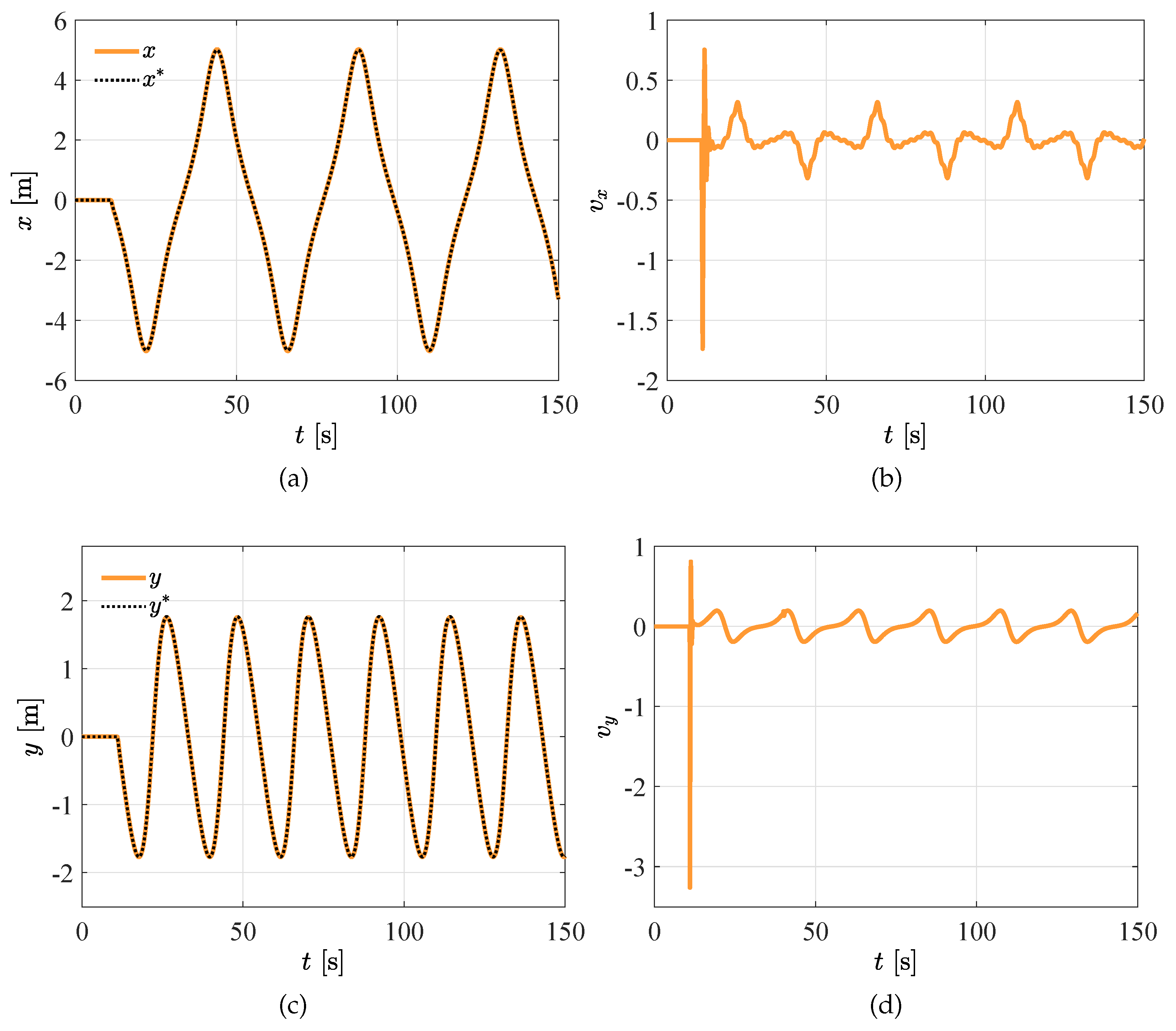
As a result of suitable feedback control design, the helicopter is able to follow the predefined lemniscate reference path within the two dimensional X-Y plane, Figure 6, as a consequence of the properly trajectory tracking shown in Figure 7.
During the experiment, it is evident that by the action of the introduced adaptive PID controllers, both fully actuated and underactuated dynamics are properly controlled.
Figure 7 depicts the close-loop response of the system underactuated dynamics, where the trajectory tracking issue is properly solved by the suitably action of the introduced virtual controllers. As aforementioned, by the regulation of the roll and pitch dynamics, it is possible to ensure the desire motion on the horizontal plane. So it can be conclude that regulation of the angular dynamics plays a fundamental role in control motion, as well as a correct selection of the expression (9) which relates the calculus of the reference angles, whose dynamics are fully actuated, with the underactuated motion.
Different operational conditions where considered for the BsNN training process, where the system is carried from an initial condition to a desired point [37]. Notice it is complicated to know the derivatives of the on-line computed references, since and are functions dependants of the dynamic controllers and , of the mass, the constant of gravity, and the actual feedback values and . Nevertheless, the adaptive structure allows to compensate adequately this absent of information.
For simplicity of results presentation, in Figure 8 it is presented only the dynamic gain values for the regulation of z position. Here, it is observed the dynamic behaviour of the control parameters which are intelligent adjusted by the use of the neural networks. The plot also shows that, in specific small time windows, the values of the control gains turns briefly to negative values, which in a fixed gain control scheme could be lead to a system unstable condition.
From figures, it is evident the effectiveness of the introduced adaptive control scheme (Figure 3) to deal with the trajectory tracking problem of a quadrotor UAV. In the study different sorts of references profiles where assigned for the fully actuated vertical motion, as well as for underactuated motion above the horizontal plane. Besides, due to the action of the adaptive gains scheme, the effects of feedback high-gain are suitably minimized, which means that the actuators will be not saturated.
Additionally, in the next section, some disturbance forces are included in order to asses the robustness of the proposed adaptive control scheme while the quadrotor is performing tracking tasks.
4.2. Adaptive Control Performance against Disturbances
For the sake of simplicity in the results presentation, only results from vertical motion are included. Nevertheless, the introduced control schemes were properly validated by several simulations for the other translational and rotational motions. Therefore, in order to simulate the possibly effects of the wind on the flying quadrotor within an uncontrolled environment (crosswinds and gusts), two different disturbance signals are injected to the system: with for both case studies, and and for the first and the second test, respectively. Besides, harmonic forces perturbing the roll and pitch dynamics are included as for .
In Figure 9 it is observed the response of the system subjected to two different disturbances. Here, the adaptive controller tries to compensate the undesired induced oscillations while tracking tasks are executed. As it is illustrated in the pictures, in spite of that the nominal adaptive control allows the quadrotor tracking the planned references, in both cases undesired motion oscillations are present. Moreover, the respective computed control inputs are not smooth. Keep in mind that due to the BsNN’s work as iterative algorithms it is possibly that in specific sceneries, with particular operational conditions, they could act as filters in presence of relative high frequency signals, which will be a discussion topic in future studies.
Notice, that the magnitude and frequency of the injected disturbance signals have significant effects on the dynamic response of the system. It is important to highlight that even in the presence of significant disturbances the control scheme is able to keep the quadrotor near of the desire reference position. Nevertheless, it is desirable that undesired oscillating motions not to be present in the system response.
It is evident that the satisfactory results achieved for the unperturbed case are quite different for both disturbed case of studies. Thus, it is necessary to consider the use of the observer mechanism for disturbance estimation, and in this fashion, take advantage of the features of both control structures.
4.3. Robust Adaptive Control Performance against Disturbances
Now, consider the following control law for the auxiliary vertical motion controller
where is the disturbance estimated by the extended observer (22). So, by substituting the Equation (25) in the disturbed version of (12) for z variable
then,
so, by assuming that , then without loss of generality, the Equation (14) is true, and the nominal controller is then responsible of tracking and regulation tasks. The observer gains are selected as , , , with for translational and for rotational dynamics, respectively.
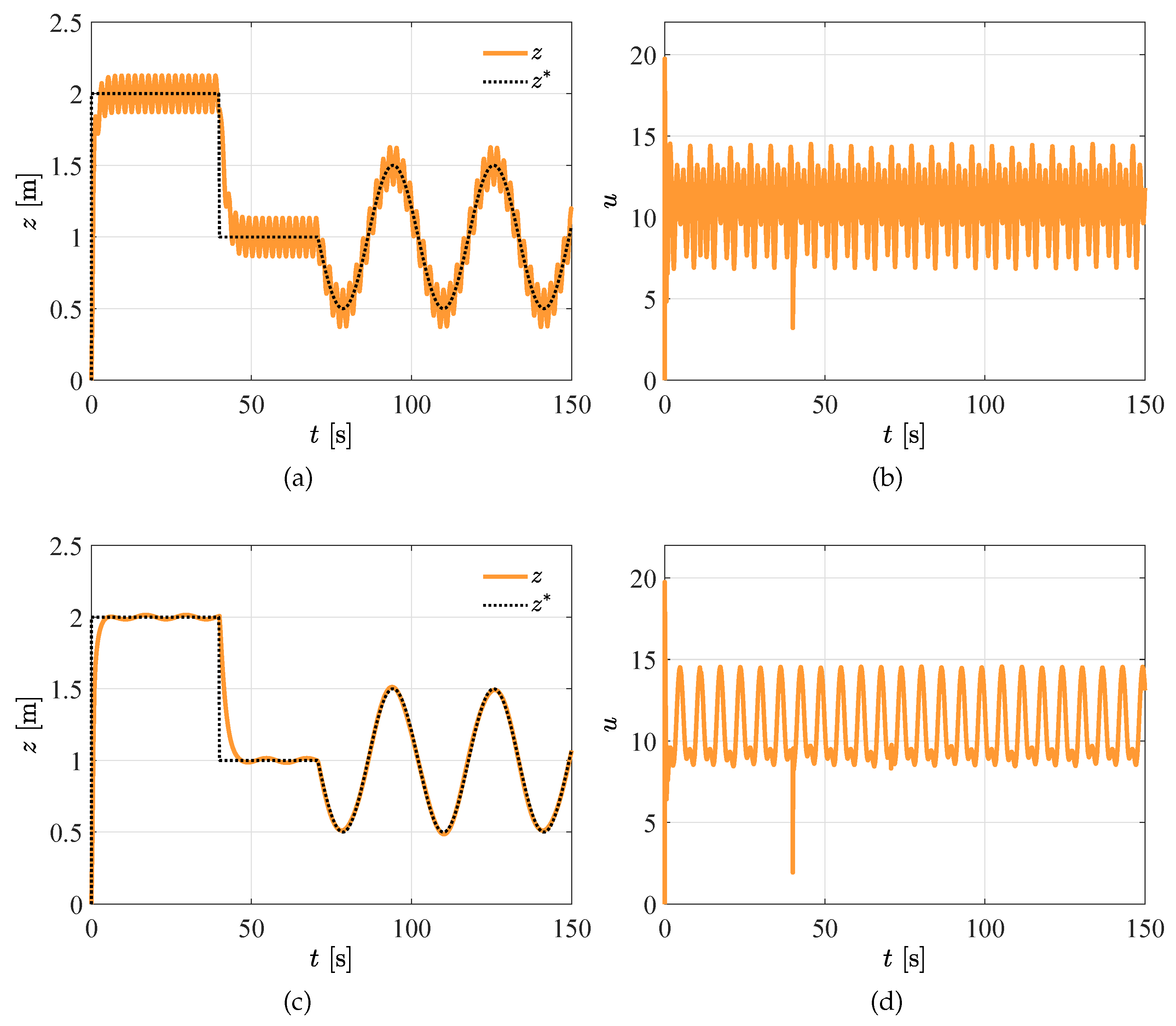
Then, as aforementioned (and previously demonstrated), the nominal optimal controller is able to perform a very good tracking and regulation. Figure 10 depicts the reference tracking for both case studies, where the proposed robust adaptive PID controller is implemented. Here, a satisfactory performance of the control scheme is observed, where even in the presence of the disturbances, the efficiency of the control action is not affected, which guarantee close-loop stability.
The main force control input u for each case study is portrayed in Figure 11, where is evident the effects of the injected compensation for actively reject the estimated disturbance . On the other hand, it is observed that the selected observer gains allows to tracking the real disturbance by the estimation. Notice, the estimated variables can be used in the controller design, or such as complementary information in the filtering stage for data collected by sensors. In the pictures related with the case study 1 in Figure 11, the time scale has been modified with purposes of improve the visualization of the yielded results. Moreover, it is shown that in spite of the oscillations present in the control signal, the motion is free from undesired oscillations.
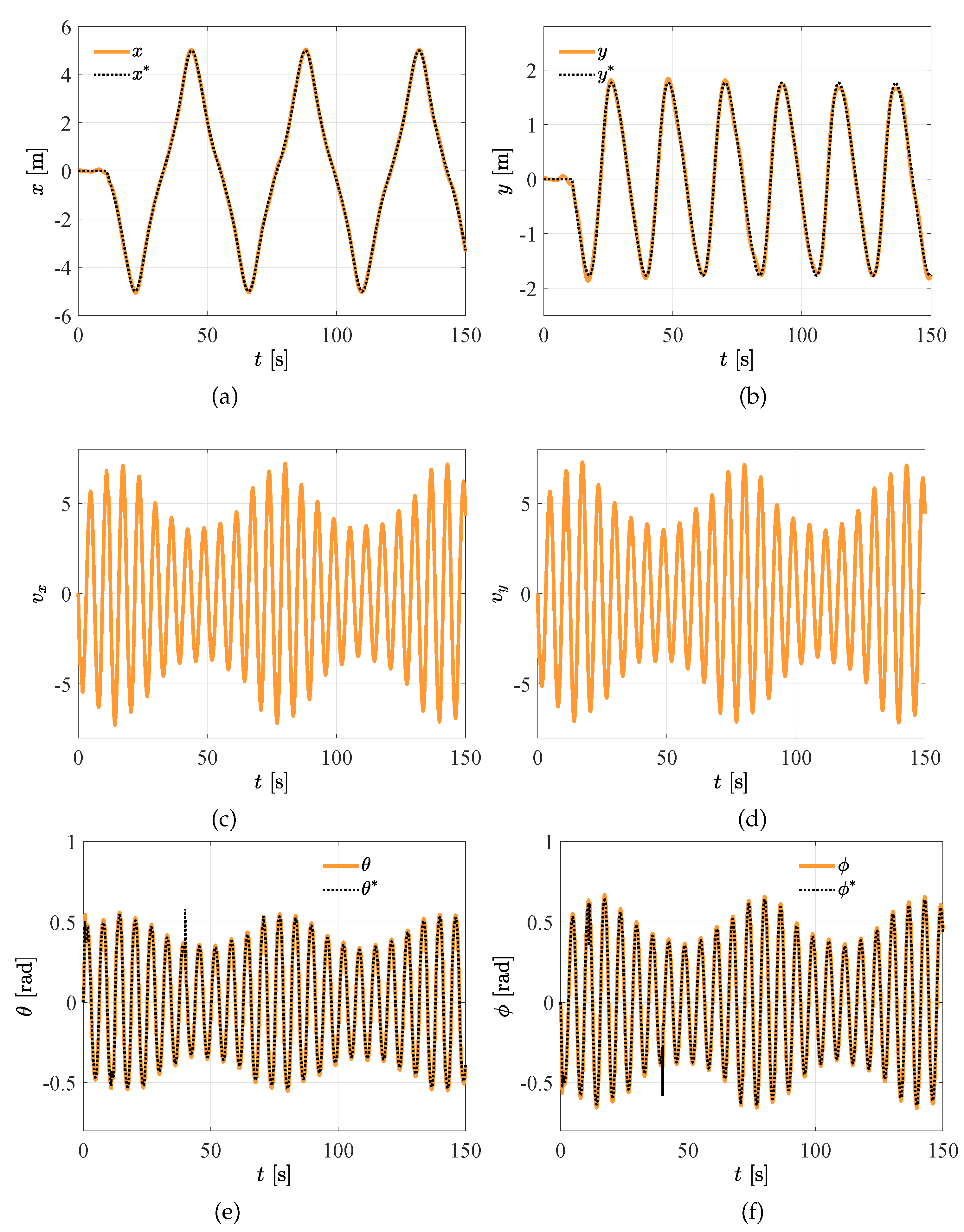
Finally, in Figure 12 it is observed the effectiveness of the introduced control strategy, where both the unperturbed and perturbed responses for the underactuated motion are depicted. Here, harmonic forces perturbing the horizontal displacements (lateral and longitudinal) are included as for , Figure 13.
Moreover, it is appreciated the control robustness to face undesired harmonic effects induced by endogenous perturbations, where only a slight deviation from the reference trajectory is observed at . Also, despite the derivatives of the on-line computed angular references are not included in the control scheme, the adaptation capabilities provided by the BsNN control allow a proper tracking of the angular dynamic references and , ensuring at the same time the planned motion on the horizontal plane. It is worth to note that the study of the design and implementation of this kind of controllers can be extended to another aerial vehicles as the fixed wing UAV.
4.4. Dynamic Response in Presence of Turbulent Wind Field
In this section the Dryden wind gust model presented in [24] is introduced to the system in order to verify the quadrotor behaviour by using the proposed controller. Here, it is assumed that the disturbance caused by wind field is proportional to the wind speed, and is defined as a set of sinusoidal excitations given by
where is a description of the wind disturbance in , or channels in a specific instant of time, meanwhile and are randomly selected frequencies and phase shifts, respectively; n is the number of sinusoids, is the amplitude, and is a static term for wind disturbance. Besides, the disturbance torque caused by the wind field is proportional to the wind speed [24]. Thus, the model (28) can be used as torque disturbances , and in (7), where the particular values considering for , are summarized in Table 3.
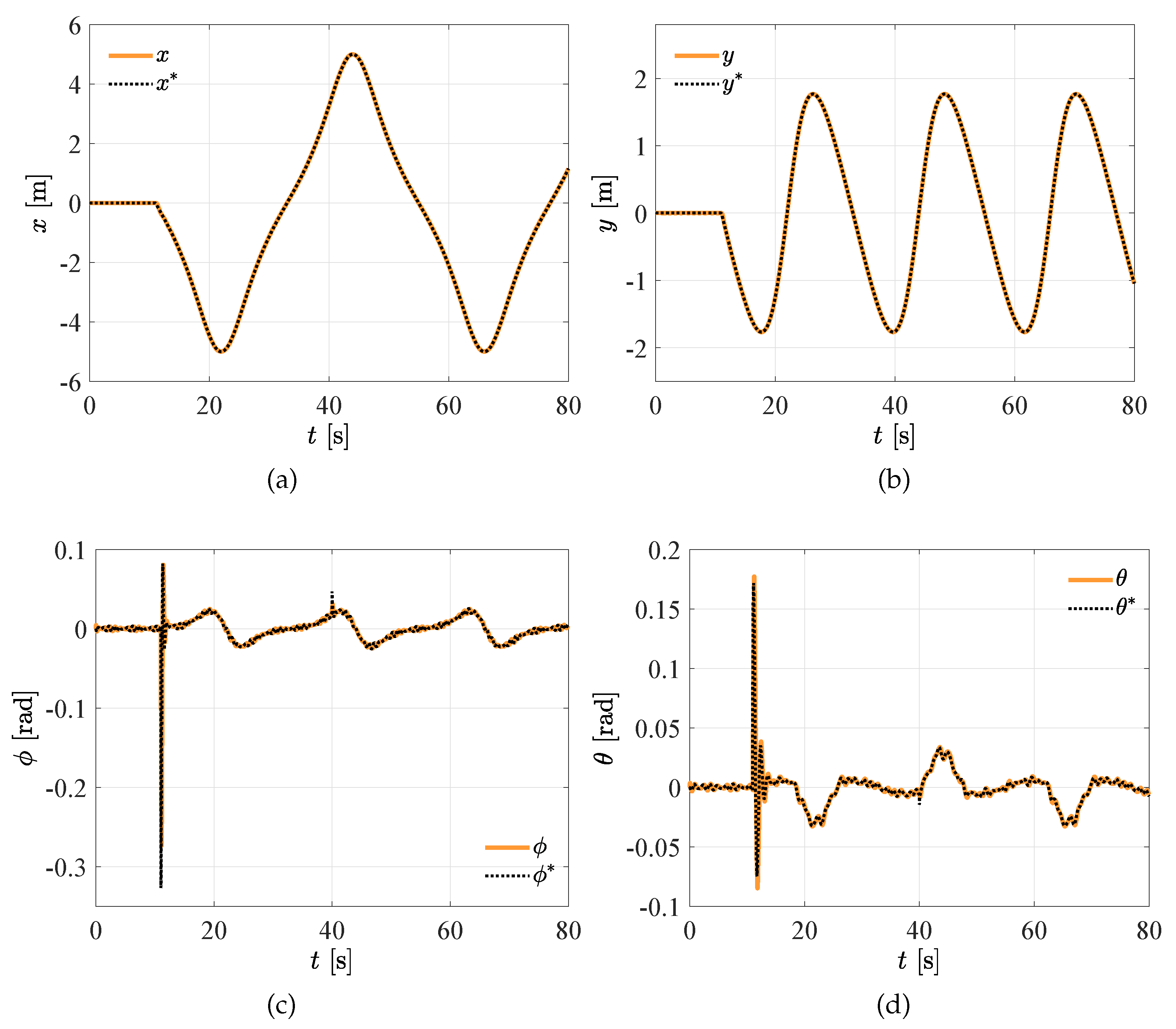
Results portrayed in Figure 14 and Figure 15 show the performance of the system while facing the disturbance torques described in Table 3. Here, the robustness capabilities of the proposed scheme allows the quadrotor following the reference trajectories.
In addition, for the sake of simplicity in the results presentation, only 80 seconds of the full time line are presented. From figures we conclude that the introduced controller is a very good alternative for deal with disturbance rejection problem while trajectory tracking tasks are perform by a quadrotor helicopter.
5. Conclusions
A novel robust adaptive neural motion control strategy for a quadrotor UAV has been introduced. Adaptive control structure has been designed using neural networks of the type B-spline, which allows to minimize significantly the high-gain feedback effects. Later, an linear extended state observer has been adopted for estimating the generalized disturbance, which is used in the main control law design for counteracting harmonic disturbing forces. Furthermore, several numeric simulations were performed to asses the robustness of the proposed control scheme, where it is confirmed a successful performance for tracking and regulation tasks while acceptable levels of disturbance attenuation are achieved. Yielded results corroborate that the proposed control strategy is an efficient alternative for motion control of disturbed nonlinear systems. Future works will be focussed on the off-line training process for the neural networks in order to improve their disturbance rejection capabilities.
Author Contributions
Research and writing, H.Y.-B., R.T.-O., F.B.-C.; and Supervision, R.T.-O., F.B.-C. All authors have read and agreed to the published version of the manuscript.
Funding
This research received no external funding.
Conflicts of Interest
The authors declare no conflict of interest. The funders had no role in the design of the study; in the collection, analyses, or interpretation of data; in the writing of the manuscript, or in the decision to publish the results.
Abbreviations
The following abbreviations are used in this manuscript:
| UAV | Unmanned Aerial Vehicle |
| FW-UAV | Fixed-Wing Unmanned Aerial Vehicle |
| RW-UAV | Rotary-Wing Unmanned Aerial Vehicle |
| VTOL | Vertical Take off and Landing |
| PID | Proportional Integral Derivative |
| MPC | Model Predictive Control |
| NLIMC | Nonlinear Internal Model Control |
| ADRC | Active Disturbance Rejection Control |
| EMC | Embedded Model Control |
| ANN | Artificial Neural Network |
| BsNN | B-spline Neural Network |
| ESO | Extended State Observer |
| LESO | Linear Extended State Observer |
References
- Siciliano, B.; Khatib, O. (Eds.) Springer Handbook of Robotics, 2nd ed.; Springer International Publishing: Cham, Switzerland, 2016. [Google Scholar]
- Castillo, P.; Lozano, R.; Dzul, A. Modelling and Control of Mini-Flying Machines, 1st ed.; Springer Publishing Company, Inc.: New York, NY, USA, 2010. [Google Scholar]
- Corke, P. Robotics, Vision and Control: Fundamental Algorithms in MATLAB, 2nd ed.; Springer Publishing Company, Incorporated: New York, NY, USA, 2017. [Google Scholar]
- Bouabdallah, S.; Noth, A.; Siegwart, R. PID vs. LQ Control Techniques Applied to an Indoor Micro Quadrotor. In Proceedings of the 2004 IEEE/RSJ International Conference on Intelligent Robots and Systems (IROS) (IEEE Cat. No.04CH37566), Sendai, Japan, 28 September–2 October 2004; Volume 3, pp. 2451–2456. [Google Scholar]
- Hoffmann, G.; Huang, H.; Waslander, S.; Tomlin, C. Quadrotor Helicopter Flight Dynamics and Control: Theory and Experiment. In AIAA Guidance, Navigation and Control Conference and Exhibit; American Institute of Aeronautics and Astronautics: Reston, VA, USA, 2007; pp. 1670–1689. [Google Scholar]
- Liu, H.; Li, D.; Zuo, Z.; Zhong, Y. Robust Three-Loop Trajectory Tracking Control for Quadrotors With Multiple Uncertainties. IEEE Trans. Ind. Electron. 2016, 63, 2263–2274. [Google Scholar] [CrossRef]
- Mian, A.A.; Daobo, W. Modeling and Backstepping-based Nonlinear Control Strategy for a 6 DOF Quadrotor Helicopter. Chin. J. Aeronaut. 2008, 21, 261–268. [Google Scholar] [CrossRef] [Green Version]
- Modirrousta, A.; Khodabandeh, M. A novel nonlinear hybrid controller design for an uncertain quadrotor with disturbances. Aerosp. Sci. Technol. 2015, 45, 294–308. [Google Scholar] [CrossRef]
- Bouabdallah, S.; Siegwart, R. Backstepping and Sliding-mode Techniques Applied to an Indoor Micro Quadrotor. In Proceedings of the 2005 IEEE International Conference on Robotics and Automation, Barcelona, Spain, 18–22 April 2005; pp. 2247–2252. [Google Scholar]
- Jia, Z.; Yu, J.; Mei, Y.; Chen, Y.; Shen, Y.; Ai, X. Integral backstepping sliding mode control for quadrotor helicopter under external uncertain disturbances. Aerosp. Sci. Technol. 2017, 68, 299–307. [Google Scholar] [CrossRef]
- Zheng, E.H.; Xiong, J.J.; Luo, J.L. Second order sliding mode control for a quadrotor UAV. ISA Trans. 2014, 53, 1350–1356. [Google Scholar] [CrossRef]
- Luque-Vega, L.; Castillo-Toledo, B.; Loukianov, A.G. Robust block second order sliding mode control for a quadrotor. J. Frankl. Inst. 2012, 349, 719–739. [Google Scholar] [CrossRef]
- Raffo, G.V.; Ortega, M.G.; Rubio, F.R. An integral predictive/nonlinear H∞ control structure for a quadrotor helicopter. Automatica 2010, 46, 29–39. [Google Scholar] [CrossRef]
- Yao, J.; Deng, W. Active disturbance rejection adaptive control of uncertain nonlinear systems: Theory and application. Nonlinear Dyn. 2017, 89, 1611–1624. [Google Scholar] [CrossRef]
- Dierks, T.; Jagannathan, S. Output Feedback Control of a Quadrotor UAV Using Neural Networks. IEEE Trans. Neural Netw. 2010, 21, 50–66. [Google Scholar] [CrossRef]
- Bouzid, Y.; Siguerdidjane, H.; Bestaoui, Y. Nonlinear internal model control applied to VTOL multi-rotors UAV. Mechatronics 2017, 47, 49–66. [Google Scholar] [CrossRef]
- Lotufo, M.A.; Colangelo, L.; Perez-Montenegro, C.; Canuto, E.; Novara, C. UAV quadrotor attitude control: An ADRC-EMC combined approach. Control Eng. Pract. 2019, 84, 13–22. [Google Scholar] [CrossRef]
- Wahid, N.; Hassan, N.; Rahmat, M.F.; Mansor, S. Aircraft Pitch Control Design using Observer-State Feedback Control. Aust. J. Basic Appl. Sci. 2011, 5, 1065–1074. [Google Scholar]
- Guo, B.Z.; Zhao, Z.L. Active Disturbance Rejection Control for Nonlinear Systems: An Introduction, 1st ed.John Wiley and Sons(Asia) Pte Ltd.: Singapore, 2016. [Google Scholar]
- Li, S.; Yang, J.; Chen, W.-H.; Cheng, X. Disturbance Observer-Based Control, 1st ed.; CRC Press, Taylor and Francis Group: Boca Raton, FL, USA, 2014. [Google Scholar]
- Sun, D. Comments on Active Disturbance Rejection Control. IEEE Trans. Ind. Electron. 2007, 54, 3428–3429. [Google Scholar]
- Li, S.; Xia, C.; Zhou, X. Disturbance rejection control method for permanent magnet synchronous motor speed-regulation system. Mechatronics 2012, 22, 706–714. [Google Scholar] [CrossRef]
- Zhao, S.; Gao, Z. An Active Disturbance Rejection Based Approach to Vibration Suppression in Two-Inertia Systems. Asian J. Control 2013, 15, 350–362. [Google Scholar] [CrossRef] [Green Version]
- Shi, D.; Wu, Z.; Chou, W. Generalized Extended State Observer Based High Precision Attitude Control of Quadrotor Vehicles Subject to Wind Disturbance. IEEE Access 2018, 6, 32349–32359. [Google Scholar] [CrossRef]
- Li, J.; Li, R.; Zheng, H. Quadrotor modeling and control based on Linear Active Disturbance Rejection Control. In Proceedings of the 2016 35th Chinese Control Conference (CCC), Chengdu, China, 27–29 July 2016; pp. 10651–10656. [Google Scholar]
- Lu, H.; Zhu, X.; Ren, C.; Ma, S.; Wang, W. Active Disturbance Rejection Sliding Mode Altitude and Attitude Control of a Quadrotor with Uncertainties. In Proceedings of the 2016 12th World Congress on Intelligent Control and Automation (WCICA), Guilin, China, 12–15 June 2016; pp. 1366–1371. [Google Scholar]
- Sanz, R.; Garcia, P.; Albertos, P. Active Disturbance Rejection by State Feedback: Experimental Validation in a 3-DOF Quadrotor Platform. In Proceedings of the 2015 54th Annual Conference of the Society of Instrument and Control Engineers of Japan (SICE), Hangzhou, China, 28–30 July 2015; pp. 794–799. [Google Scholar]
- Dong, W.; Gu, G.Y.; Zhu, X.; Ding, H. A high-performance flight control approach for quadrotors using a modified active disturbance rejection technique. Robot. Auton. Syst. 2016, 83, 177–187. [Google Scholar] [CrossRef]
- Shao, X.; Meng, Q.; Liu, J.; Wang, H. RISE and disturbance compensation based trajectory tracking control for a quadrotor UAV without velocity measurements. Aerosp. Sci. Technol. 2018, 74, 145–159. [Google Scholar] [CrossRef]
- Castillo, P.; García, P.; Lozano, R.; Albertos, P. Modelado y estabilización de un helicóptero con cuatro rotores. Rev. Iberoam Autom. Inform. Ind. RIAI 2007, 4, 41–57. [Google Scholar] [CrossRef] [Green Version]
- Bouabdallah, S.; Siegwart, R. Full Control of a Quadrotor. In Proceedings of the 2007 IEEE/RSJ International Conference on Intelligent Robots and Systems, San Diego, CA, USA, 29 October–2 November 2007; pp. 153–158. [Google Scholar]
- Kushleyev, A.; Mellinger, D.; Powers, C.; Kumar, V. Towards a swarm of agile micro quadrotors. Auton. Robots 2013, 35, 287–300. [Google Scholar] [CrossRef]
- Spong, M.; Hutchinson, S.; Vidyasagar, M. Robot Modeling and Control, 2nd ed.; Wiley: Hoboken, NJ, USA, 2020. [Google Scholar]
- Arnol’d, V.I. Mathematical Methods of Classical Mechanics; Springer: New York, NY, USA, 2013; Volume 60. [Google Scholar]
- Goldstein, H.; Poolef, C.; Safko, J. Classical Mechanics, 3rd ed.; Addison Wesley: New York, NY, USA, 2000. [Google Scholar]
- Brown, M.; Harris, C. Neurofuzzy Adaptive Modelling and Control; Prentice Hall International (UK) Ltd.: Hertfordshire, UK, 1994. [Google Scholar]
- Yañez-Badillo, H.; Tapia-Olvera, R.; Aguilar-Mejia, O.; Beltran-Carbajal, F. Control Neuronal en Línea para Regulación y Seguimiento de Trayectorias de Posición para un Quadrotor. Rev. Iberoam. Autom. Inform. Ind. RIAI 2017, 14, 141–151. [Google Scholar] [CrossRef] [Green Version]
- Saad, D. (Ed.) On-line Learning in Neural Networks; Cambridge University Press: New York, NY, USA, 1998. [Google Scholar]
- Beltran-Carbajal, F.; Tapia-Olvera, R.; Valderrabano-Gonzalez, A.; Lopez-Garcia, I. Adaptive neuronal induction motor control with an 84-pulse voltage source converter. Asian J. Control 2020. [Google Scholar] [CrossRef]
- Han, J. From PID to Active Disturbance Rejection Control. IEEE Trans. Ind. Electron. 2009, 56, 900–906. [Google Scholar] [CrossRef]
- Gao, Z. Active Disturbance Rejection Control: A Paradigm Shift in Feedback Control System Design. In Proceedings of the 2006 American Control Conference, Minneapolis, MN, USA, 14–16 June 2006; pp. 2399–2405. [Google Scholar]
- Weisstein, E.W. Lemniscate. Available online: https://mathworld.wolfram.com/Lemniscate.html (accessed on 17 July 2020).
Figure 1.
A flying quadrotor subjected to main four control inputs.
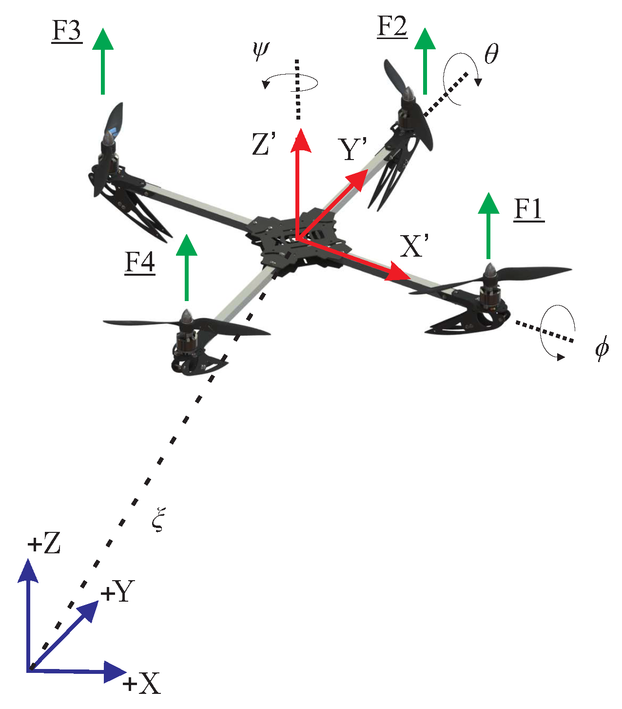
Figure 2.
B-spline network structure.

Figure 3.
Adaptive neural controller diagram.
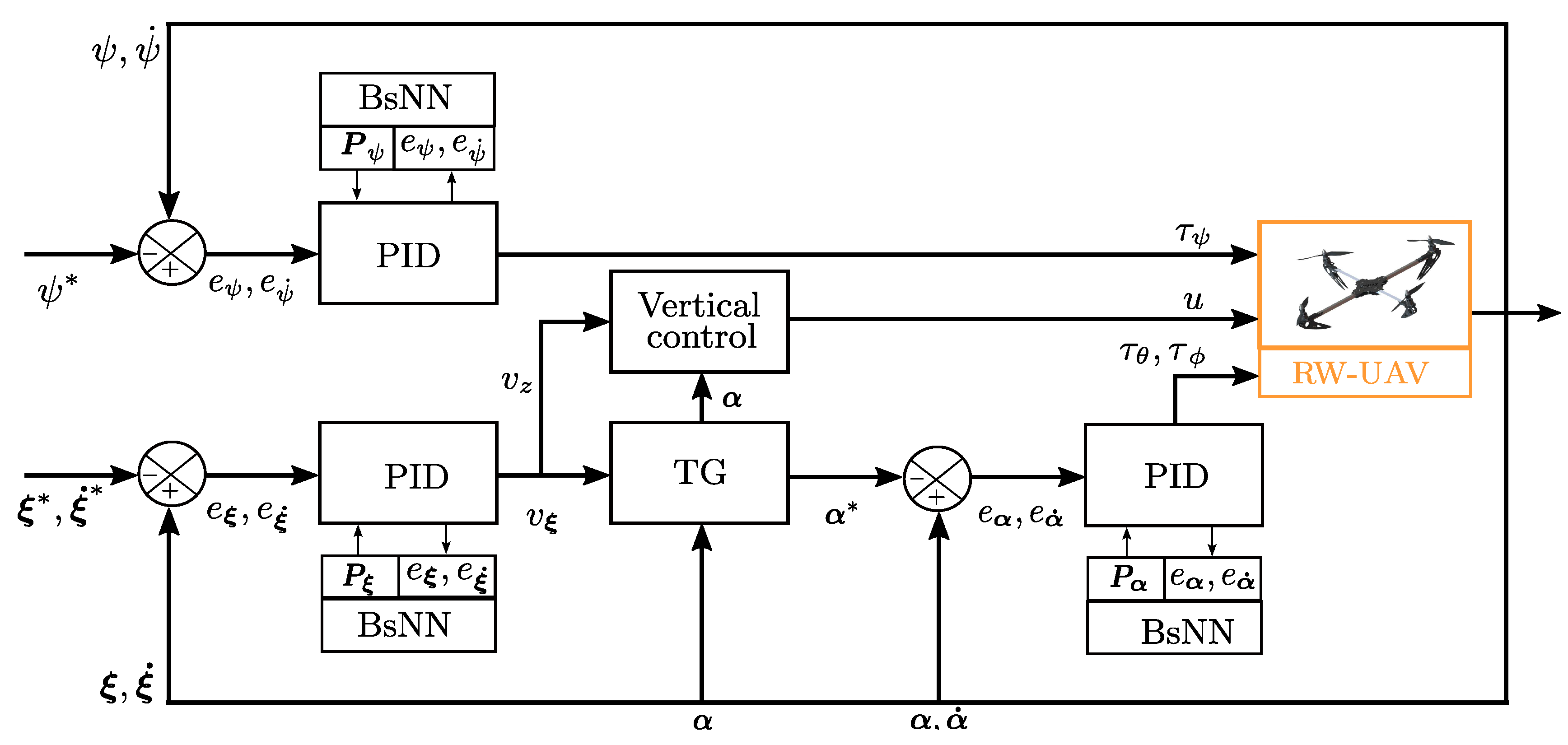
Figure 4.
Controlled vertical dynamics. (a) Tracking of the desired vertical position. (b) Main trust force control input u. (c) Yaw angle regulation. (d) Computed input control .
Figure 4.
Controlled vertical dynamics. (a) Tracking of the desired vertical position. (b) Main trust force control input u. (c) Yaw angle regulation. (d) Computed input control .
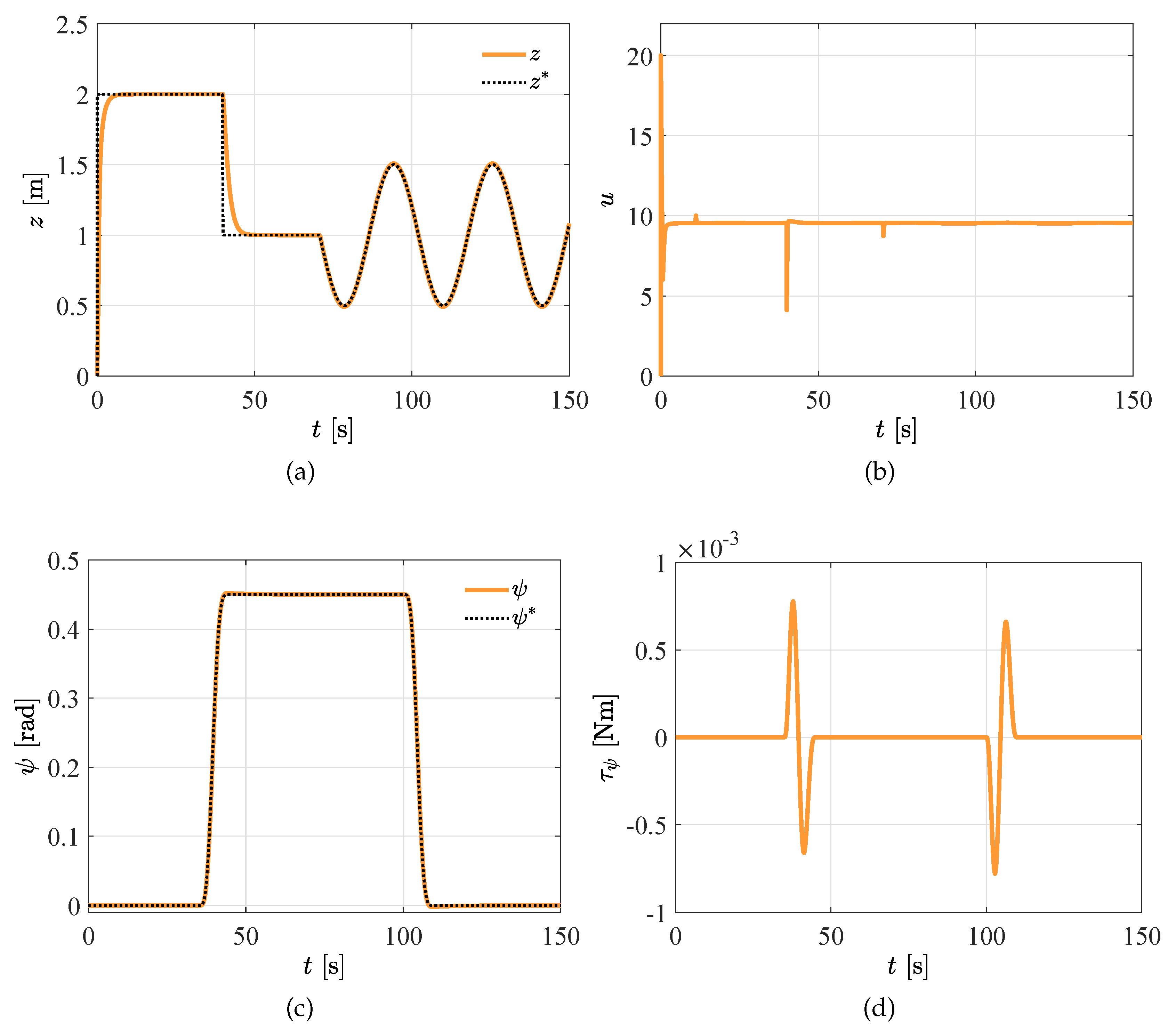
Figure 5.
Pitch and roll dynamics.(a) Tracking of the desired angle. (b) Tracking of the desired angle. (c) Computed input control . (d) Computed input control .
Figure 5.
Pitch and roll dynamics.(a) Tracking of the desired angle. (b) Tracking of the desired angle. (c) Computed input control . (d) Computed input control .

Figure 6.
Path following on the horizontal plane.

Figure 7.
Controlled underactuated dynamics. (a) Tracking of the desired x position. (b) Virtual controller . (c) Tracking of the desired y position. (d) Virtual controller .
Figure 7.
Controlled underactuated dynamics. (a) Tracking of the desired x position. (b) Virtual controller . (c) Tracking of the desired y position. (d) Virtual controller .

Figure 8.
On-line computed adaptive control parameters for vertical motion.(a) Derivative gain . (b) . (c) Proportional gain . (d) . (e) Integral gain . (f) .
Figure 8.
On-line computed adaptive control parameters for vertical motion.(a) Derivative gain . (b) . (c) Proportional gain . (d) . (e) Integral gain . (f) .
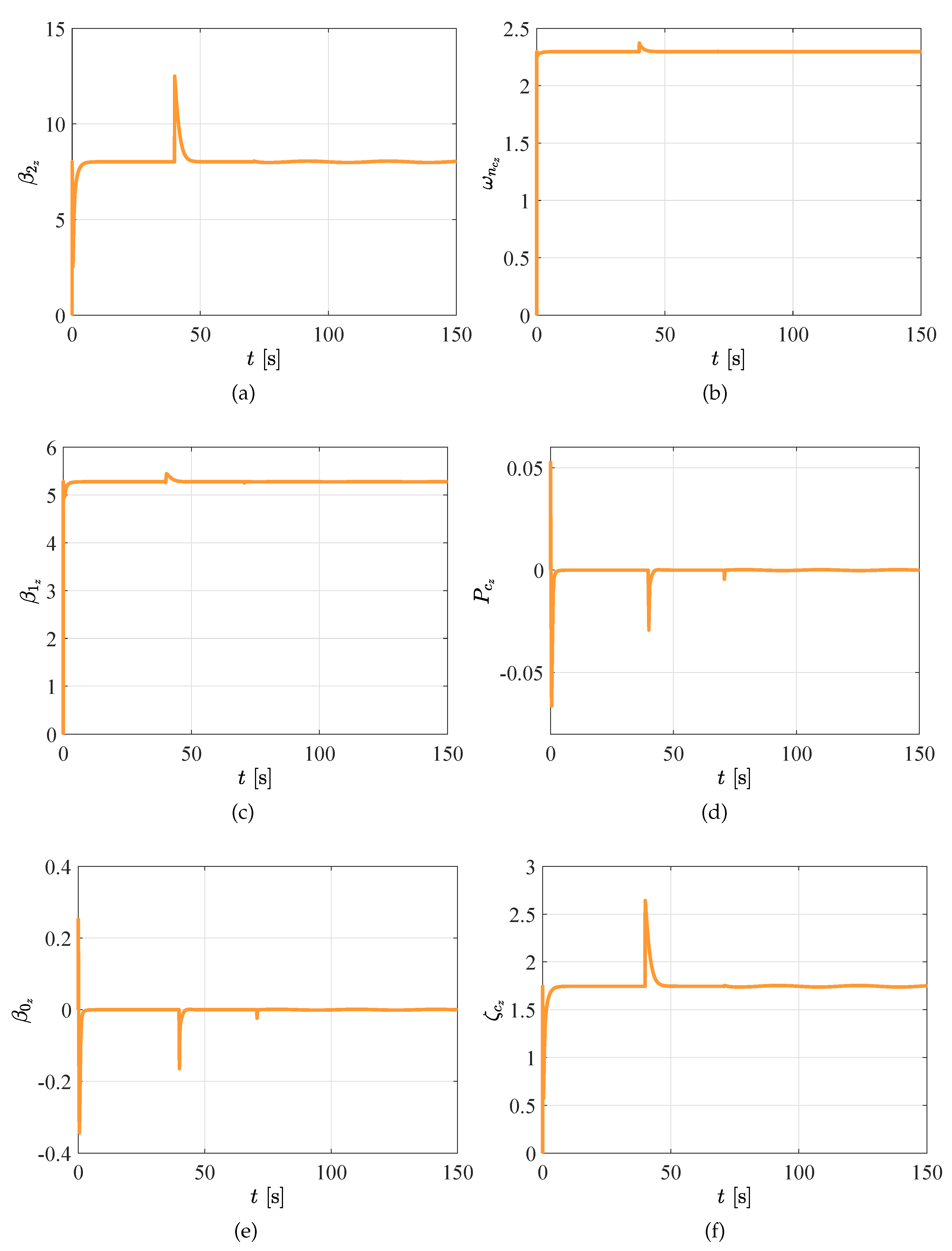
Figure 9.
Close-loop response for disturbed vertical motion by using adaptive control. (a) Tracking of the desired z position, case study 1. (b) Input control force, case study 1. (c) Tracking of the desired z position, case study 2. (d) Input control force, case study 2.
Figure 9.
Close-loop response for disturbed vertical motion by using adaptive control. (a) Tracking of the desired z position, case study 1. (b) Input control force, case study 1. (c) Tracking of the desired z position, case study 2. (d) Input control force, case study 2.

Figure 10.
Disturbed vertical motion by using robust adaptive control. (a) Tracking of the desired z position, case study 1. (b) Tracking of the desired z position, case study 2.
Figure 10.
Disturbed vertical motion by using robust adaptive control. (a) Tracking of the desired z position, case study 1. (b) Tracking of the desired z position, case study 2.
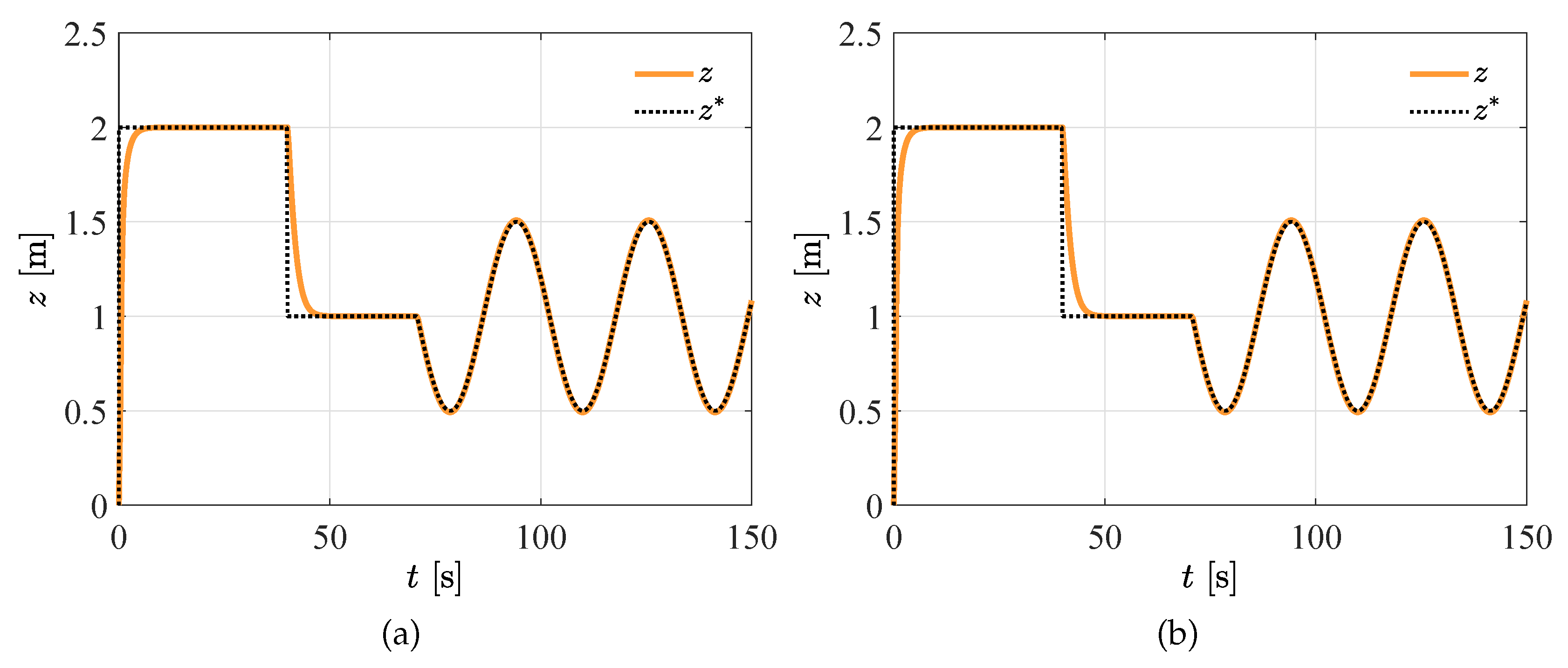
Figure 11.
Close-loop response for disturbed vertical motion by using robust adaptive control. (a) Tracking of the desired z position, case study 1. (b) Estimated disturbance by LESO, case study 1. (c) Tracking of the desired z position, case study 2. (d) Estimated disturbance by LESO, case study 2.
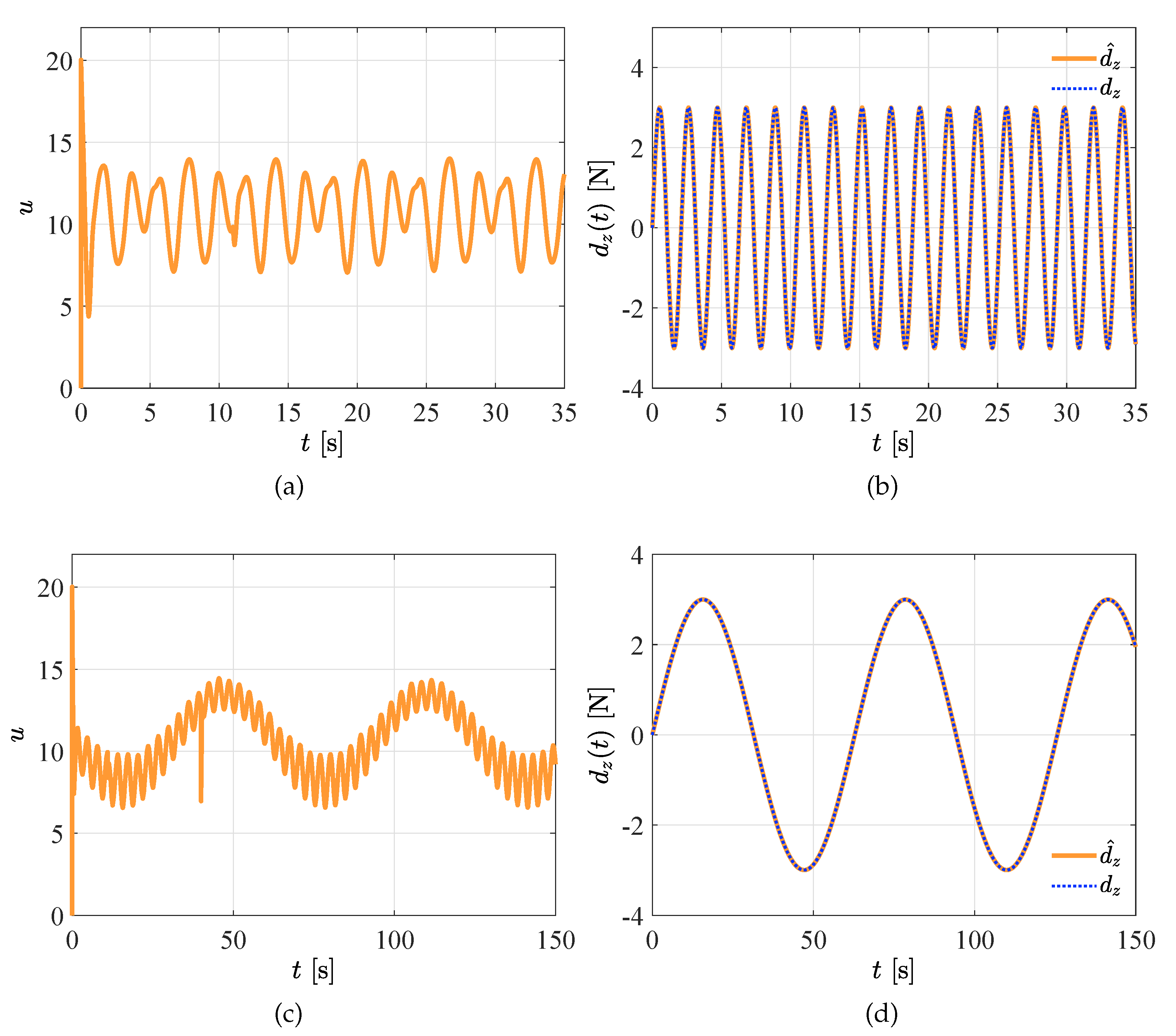
Figure 12.
Disturbed underactuated dynamics. (a) Tracking of the desired x position. (b) Virtual controller . (c) Tracking of the desired y position. (d) Virtual controller . (e) Tracking of the desired angle. (f) Tracking of the desired angle.
Figure 12.
Disturbed underactuated dynamics. (a) Tracking of the desired x position. (b) Virtual controller . (c) Tracking of the desired y position. (d) Virtual controller . (e) Tracking of the desired angle. (f) Tracking of the desired angle.

Figure 13.
Horizontal injected disturbances. (a) Lateral. (b)Longitudinal.
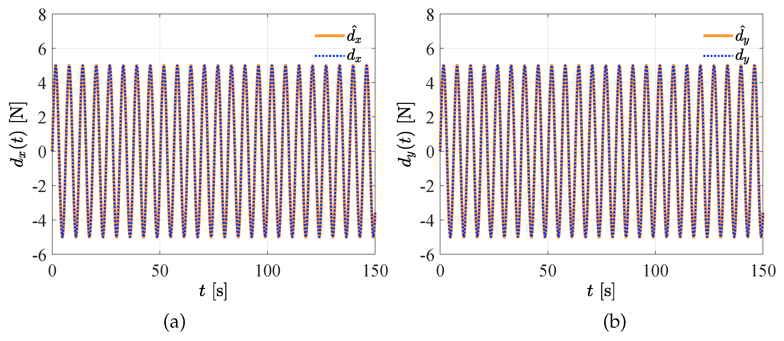
Figure 14.
Disturbed dynamics. (a) Tracking of the desired x position. (b) Tracking of the desired y position. (c) Tracking of the desired angle. (d) Tracking of the desired angle.
Figure 14.
Disturbed dynamics. (a) Tracking of the desired x position. (b) Tracking of the desired y position. (c) Tracking of the desired angle. (d) Tracking of the desired angle.

Figure 15.
Dynamic response in presence of turbulent wind field. (a) . (b) Estimation of the disturbance torque . (c) . (d) Estimation of the disturbance torque . (e) . (f) Estimation of the disturbance torque .
Figure 15.
Dynamic response in presence of turbulent wind field. (a) . (b) Estimation of the disturbance torque . (c) . (d) Estimation of the disturbance torque . (e) . (f) Estimation of the disturbance torque .

Table 1.
Planned references for horizontal displacements.
| References | Units | ||
|---|---|---|---|
| m | 0 | ||
| m/s | 0 | ||
| m/s2 | 0 | ||
| m | 0 | ||
| m/s | 0 | ||
| m/s2 | 0 |
Table 2.
Planned references for vertical motion.
| References | Units | |||
|---|---|---|---|---|
| m | 2 | 1 | ||
| m/s | 0 | 0 | ||
| m/s2 | 0 | 0 |
Table 3.
Particular values for disturbances.
| 0.3 | ||||
| 0.6 | ||||
| 2 |
© 2020 by the authors. Licensee MDPI, Basel, Switzerland. This article is an open access article distributed under the terms and conditions of the Creative Commons Attribution (CC BY) license (http://creativecommons.org/licenses/by/4.0/).
Share and Cite
MDPI and ACS Style
Yañez-Badillo, H.; Tapia-Olvera, R.; Beltran-Carbajal, F. Adaptive Neural Motion Control of a Quadrotor UAV. Vehicles 2020, 2, 468-490. https://0-doi-org.brum.beds.ac.uk/10.3390/vehicles2030026
AMA Style
Yañez-Badillo H, Tapia-Olvera R, Beltran-Carbajal F. Adaptive Neural Motion Control of a Quadrotor UAV. Vehicles. 2020; 2(3):468-490. https://0-doi-org.brum.beds.ac.uk/10.3390/vehicles2030026
Chicago/Turabian StyleYañez-Badillo, Hugo, Ruben Tapia-Olvera, and Francisco Beltran-Carbajal. 2020. "Adaptive Neural Motion Control of a Quadrotor UAV" Vehicles 2, no. 3: 468-490. https://0-doi-org.brum.beds.ac.uk/10.3390/vehicles2030026