The Association of Media and Environmental Variables with Transit Ridership


1
Department of City & Metropolitan Planning, University of Utah, Salt Lake City, UT 84112, USA
2
Department of Atmospheric Sciences, University of Utah, Salt Lake City, UT 84112, USA
3
NEXUS Institute, University of Utah, Salt Lake City, UT 84112, USA
4
Department of Political Science, University of Utah, Salt Lake City, UT 84112, USA
*
Author to whom correspondence should be addressed.
Vehicles 2020, 2(3), 507-522; https://0-doi-org.brum.beds.ac.uk/10.3390/vehicles2030028
Submission received: 4 July 2020
/
Revised: 8 August 2020
/
Accepted: 11 August 2020
/
Published: 12 August 2020
Abstract
:Transportation systems are central to all cities, and city planners and policy makers take special interest in assuring these systems are efficient, functional, sustainable, and, increasingly, that they have a positive impact on human health. In addition, vehicular emissions are increasingly costly to cities due to congestion and its impact on public health. This study aims to show the associations between the media and environmental variables and associated transit ridership. By tracking media influence, we illustrated how media coverage and attention to an issue over time may impact public opinion and ridership outcomes, especially at the local level where the issues are most salient. The relationship between air quality and transit ridership shown can be generally explained through a combination of infrastructure and human behavior. The media key terms examined in this analysis show that ridership is associated with favorable weather conditions and air quality, suggesting that ridership volume may be influenced by an overall sense of comfort and safety. Based on this analysis, we illustrated the role of media attention in both increased and decreased transit ridership and how such effects are compounded by air quality conditions (e.g., green, yellow, orange, and red air quality days).
1. Introduction
1.1. Motivation
Transportation systems are central to all cities because of the various functions they provide. Public transit in particular encourages economic activity by enabling the mobility of consumers and lower income workers. Public ridership can also reduce environmental externalities such as congestion and pollution by offsetting personal vehicle usage. In addition, vehicular emissions are increasingly costly to cities due to congestion and a range of health-related impacts. For instance, transportation makes up about 75 percent of all CO2 emissions and around 28 percent of total greenhouse gas emissions found in US cities [1]. Public transportation, therefore, is critical for the long-term viability of any large urban area, and policy makers take special interest in assuring these systems are efficient, functional, sustainable, and, increasingly, that they have a positive impact on human health. Subsequently, a range of work has emerged on policy determinants and incentives to encourage public ridership. One determinant of increasing interest is the role that media can play in both promoting and deterring ridership. We intend to contribute to this discussion by exploring whether media attention to local air quality and meteorological conditions have any impacts on transit ridership.
To explore this relationship, we study media key term usage across a range of meteorological and air quality conditions and their association with ridership on the Utah Transit Authority (UTA) service area in Utah (USA) from 1 January 2014 to 31 December 2016. We also aim to understand if ridership is further associated with the Utah Division of Air Quality’s (UDAQ) “air quality (AQ) days” systems that rate local air quality by red (worst), orange, yellow, or green air quality each day. Based on this analysis, we hope to understand if strong media attention on an upcoming meteorological event (e.g., winter storm) has a relationship with UTA ridership and whether this effect varies across green, yellow, orange, and red AQ days.
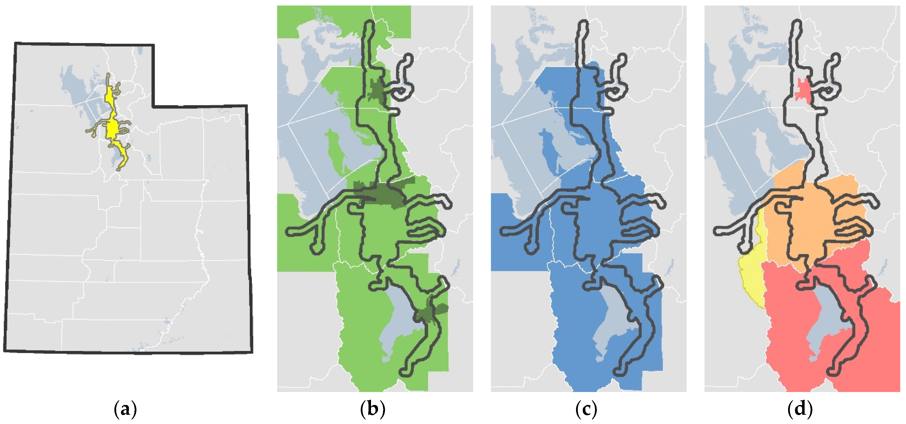
UTA provides public transportation to a seven-county area, primarily within Utah’s Wasatch Front (Figure 1). This area faces significant air quality challenges both in winter, due to elevated fine particulate matter (PM2.5) [2,3,4], and summer due to elevated ozone levels [5,6]. Other pollutants, including carbon monoxide (CO), sulfur dioxide (SO2), and coarse particulate matter (PM10), have also been found to be in excess of national ambient air quality standards (NAAQS) by the Utah Division of Air Quality (DAQ) (Figure 1) [7]. Among the mitigation strategies, the Utah Department of Transportation (UDOT) has implemented the “Clear the Air Challenge” during periods of elevated pollution [8] to encourage a reduction of personal vehicle use and increase in transit use or telecommuting. Efforts to incentivize ridership further during poor air quality events is of great importance to the effective management of the local transportation system.
1.2. Previous Work
The relationship between public transit ridership, air quality, and human behavior is becoming progressively more connected. For example, the type and design of transportation systems are increasingly studied due to the insights they provide for greater ridership. Sun et al. [10] used city-level data from China to show how increased public ridership is an efficient policy intervention and also a cost-effective way to reduce urban air pollution. This causal influence may be circular in some circumstances, as shown by the impact of strict driving restrictions on acceptance of public transport [11]. However, the authors found that attitudes toward ridership, and public transit more generally, have a large impact on policy acceptance. Inefficiencies in the transportation system, such as longer commutes and extensive connections, can also result in greater policy pushback and can lead to policy underperformance. Finally, public transit vehicles are increasingly used as a platform for on-board mobile sensing networks. Such networks can produce real-time environmental and road traffic information along with guidance for passengers and fleet managers, which drastically improves overall system efficiency [12]. The additional information provided to customers, therefore, can have significant impacts on ridership—for better or worse.
The wider literature on transit ridership has also focused in depth on the factors that can influence the level of transit ridership (e.g., physical environment, weather conditions, type of transit and stations, and various seasonality issues—season, year, month, day of week, specific holidays). Population density, levels of private vehicle ownership, topography, freeway network extent, parking availability and cost, transit network extent and service frequency, transit fares, and transit system safety and cleanliness all play a role. However, the relative importance of these various factors and the interaction between them are not well understood. In a meta study of ridership factors, Taylor and Fink [13] found that due to the extensive heterogeneity of cities worldwide, the list of factors that impact ridership were extensive, but not uniformly applied to each case. Other authors have focused on single factors such as population density, levels of private vehicle ownership, topography, freeway network capacity, parking availability and cost, transit network infrastructure and service frequency, transit fares, and transit system safety and cleanliness. For instance, Gutiérrez et al. [14] studied transit ridership at the station level to calculate a measure for “distance-decay”, which illustrates how poorly managed time tables, excessive connections, and distance to a local station can diminish ridership. Similarly, Mendoza et al. [9] explored the impact of air quality on ridership in urban settings.
Another important factor in explaining ridership outcomes is media effects or influence. Media influence occurs when mediated communication implicitly or explicitly shapes social and behavioral outcomes. The role of media influence on society is well established across a range of disciplines and topics [15,16]. Wakefield et al. [17], for instance, reviewed the outcomes of mass media campaigns in the context of various health-risk behaviors (e.g., use of tobacco, alcohol, and other drugs, heart disease risk factors, sex-related behaviors, road safety, cancer screening and prevention, child survival, and organ or blood donation) and concluded that mass media campaigns can produce positive changes or prevent negative changes in health-related behaviors across large populations. Through their work, Wakefield et al. [17] highlighted the direct and indirect mechanisms by which media can be used to change individual behavior. Directly, media influences individuals by providing information on the new norm of desirable behavior [18]. This information can be descriptive or prescriptive [19]. By doing so, the media shape individuals’ attitude and beliefs about certain actions and therefore creates societal norms [20,21,22]. Additionally, the media provide individuals with the tools to properly conform to the newly advised behavior [23].
Indirectly, media impact human behavior through two pathways. First, the media have an agenda-setting influence on institutions, which then directly influences the public [24,25,26]. Institutions such as legislative bodies (e.g., Congress), enforcement agents (e.g., the police), or religious institutions influence behavior by disseminating the message to social circles and ensuring compliance by placing material constraints and incentives. Second, the media promote social diffusion of the norms on correct action [27]. This occurs explicitly, when the media promulgate individuals to spread the important message to their social circles [23]. It also occurs tacitly as the norm naturally diffuses through interpersonal communication within families and social networks [28,29].
Media impacts on ridership specifically can be both positive and negative. For instance, Liu et al. [30] found that positive social media campaigns can greatly increase ridership, while Boisjoly et al. [31] found that transit messaging in the media and unreliable transportation scheduling websites could both lead to reduced ridership in some cases. Media influence, as a two-part framework with information selectivity, can also be used to explain mob mentality in online media platforms [32]. Media impacts on ridership and other forms of human behavior are most effective when the desired action is a “one-off” demand rather than a habitual, life-style change [17]. There is debate in the literature on whether media as a direct mechanism of behavioral change or media as an agenda setting tool on the institutions are more effective [25]. Outside of ridership, the scholarship on health-related behavioral change has focused on issues such as drug use, smoking, and preventable diseases [33,34]. Additionally, there is specific research that focuses on the media’s ability to mitigate the spread of pandemics [35,36]. Overall, media can be an effective, inexpensive tool to influence human behavior in a majority of the population, although sustained efforts are required for the intervention to be lasting.
As described further below, to measure media influence on ridership in this research, we use daily media counts as a percentage of total media, which are drawn from regional media sources for key terms related to air quality and meteorology. To better understand ridership behaviors, we use data drawn from the UTA system. In addition to cash and voucher payments, UTA services use an on/off electronic fare collection system where a user “taps on” with their transport card when boarding and “taps off” when alighting. These data are collected for each passenger trip and provide necessary information, such as temporal and spatial demand, to inform UTA for service improvement decisions and have been used in a previous study to estimate the impact of UTA vehicles on air quality in its service area [9].
1.3. This Study
This study aims to show the associations between the media and environmental variables and associated transit ridership. By tracking media influence, we intend to illustrate how media coverage and attention to an issue over time may affect public opinion and ridership outcomes, especially at the local level where the issues are most salient.
2. Materials and Methods
The study period for this analysis is 2014–2016, and the study location is the entirety of the UTA service area (Figure 1).
2.1. Media Data
To study media influence, we tracked key terms related to air quality (e.g., ozone, red air day) and meteorology (e.g., sunny, winter storm) to better understand if they influenced ridership. Table 1 provides a list of key terms that were included in this analysis. Media influence is measured using media daily topic counts of the specified terms from 40 online, Utah media sources. Our analysis uses the percentage of total news attention of the search term, which is normalized by total daily news. We chose percentage of news over absolute daily counts to avoid data effects from the weekly news cycle and to allow more consistent comparison across topics and time periods.
To gather media attention and coverage data on the proposed search terms across a range of media sources, we used Media Cloud, which is an open-source platform that tracks the contents of online news and enables researchers to track the spread of memes, media framings, and the tone of coverage of different stories [37]. This platform for studying media ecosystems was created through a joint project between the MIT Center for Civic Media and the Berkman Klein Center for Internet & Society at Harvard University. Media Cloud aggregates data from over 50,000 news sources from around the world and in over 20 languages including Spanish, French, Hindi, Chinese, and Japanese. Terms for this research were searched using the Media Cloud’s open-source database, which covered 40 Utah based media sources from 1 January, 2014 to 31 December, 2016. Media types include print native, video broadcasts, and digital native formats and cover a range of political spectrums. Table 2 and the Supplementary Materials Table S1 list the media sources and characteristics of the sources used in this research.
2.2. Meteorological and Air Quality Data
The meteorological data were obtained from the MesoWest network [38] using the Salt Lake City Airport (KSLC) as a reference point for daily high and low temperatures as well as 24-h precipitation. The Air Quality Index (AQI) [39] data were retrieved from the United States Environmental Protection Agency’s (USEPA) air quality database [40].
2.3. Public Transit Data
The transit data were obtained from UTA for the study period and included fields identifying the mode of transit used, day, time, and location, for both the starting and end points for each trip. UTA operates seven transit modes: (1) regular bus, (2) Express Bus, (3) Ski Bus, (4) Park City Bus (connecting Salt Lake City and Park City), (5) FrontRunner (commuter rail extending from the northernmost to southernmost service areas, (6) TRAX (electric light rail serving only Salt Lake County), and (7) Streetcar (limited service central light-rail line). The regular bus (“bus”), FrontRunner, and TRAX were used in this analysis as they account for the majority of the ridership, are not seasonal, and operate throughout the day.
Trips were classified into commute and non-commute trips, during weekdays, and weekend trips. The commute time period was defined as trips boarding between 6:00 and 8:59 a.m. and 3:00 and 6:00 p.m., with non-commute trips taking place outside these hours. This distinction follows previous studied time periods [9] and allows for a differentiation between non-discretionary (i.e., commuting) and discretionary trips. Transit ridership showed consistent drops during state and federal holidays (both actual and observed days), as well as during the weeks of Christmas and New Year’s Day, so these data were removed from the analysis.
2.4. Statistical Analysis
We analyze the relationship between media key term frequency on transit ridership using a linear regression between the two variables across three time scales: annual, seasonal, and monthly. To study the association of air quality with transit ridership data, we compared ridership in a pair-wise manner for each air quality index day using a t-test and report p-values. The media data were lagged by a day with respect to the meteorological and ridership data. This was done because it was determined that the public generally pays attention to weather forecasts for the following day to inform their behavior.
3. Results
The results of our analysis focused on three separate relationships. First, we explore the association between meteorological conditions and media attention. Next, we explore the relationship between media influence on ridership. We conclude with results on air quality events and ridership. The total days during the study period that correspond to each AQI level are shown in Supplementary Materials Table S2, the results are displayed by month, season (winter = December, January, February; spring = March, April, May; summer = June, July, August; fall = September, October, November), as annual totals, and as an annual average of study days for each temporal bin. Each year, approximately 344 days were studied, with the majority of dropped data occurring during the winter (e.g., December and January) because of the holiday season.
3.1. Association between Meteorological Conditions and Media Stories
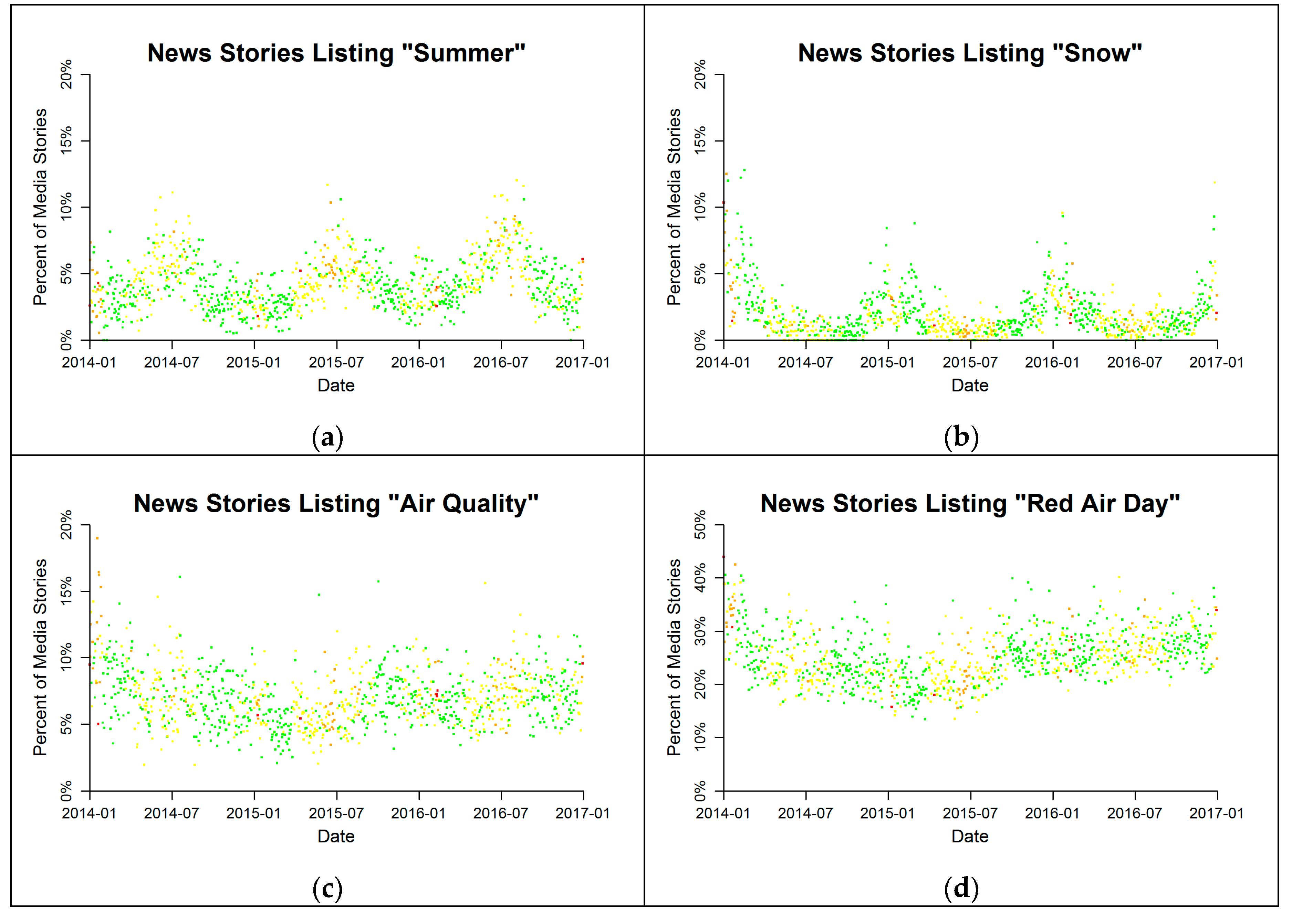
The relationship between frequency of media attention and seasons, meteorological conditions, and air quality is shown in Figure 2. The colors of the points reflect the air quality index for each data point (study day). The key terms shown were selected to illustrate the range and variety of findings. Summer (Figure 2a) shows a consistently seasonal cycle associated with the summer season. Snow (Figure 2b) is also seasonal, associated with the winter months, but reflects the sporadic nature of snowstorms. “Air quality” and “Red Air Day” (Figure 2c,d) are generally winter concerns, due to atmospheric inversions trapping pollutants, but in 2016, the terms remained consistent through the year. Overall, 2016 was a particularly active wildfire year with over 99,000 acres of burn, in comparison to 2015 and 2014 that had 10,000 and 28,000 acres of burn, respectively [41]. It is also noteworthy that while “summer”, “snow”, and “air quality” peaked at appearing in approximately 20% of news stories, “Red Air Day” peaked at 43% underlining the concern Utah has regarding unhealthy levels of pollution.
3.2. Media and Transit Ridership
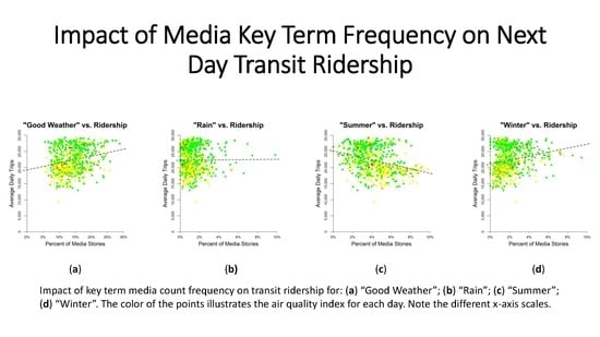
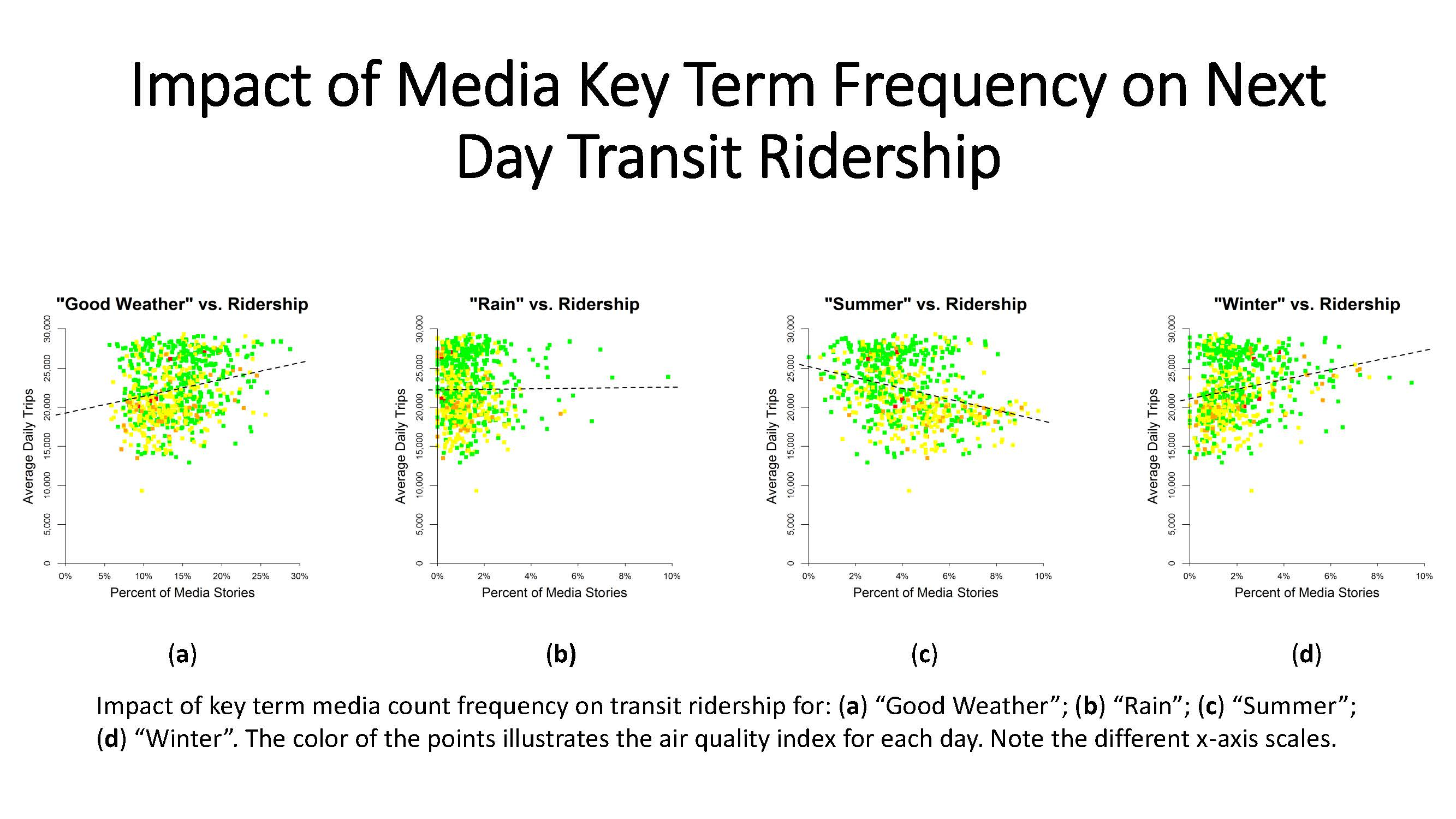
Figure 3 shows the relationship between media mentions of key terms and ridership across all transit modes the following day for all days of the year. The relationships were not found to be statistically significant for any key term, but the linear trends are shown for each figure. Figure 3a shows that there is a generally positive association with increased media mentions of “good weather” and increased ridership. “Rain” seems to have no direct effect on ridership (Figure 3b). Unsurprisingly, “summer” (Figure 3c) and “winter” (Figure 3d) show opposite trends, with the former associated with lower ridership and the latter with higher ridership.
The winter and summer seasonal differences in media term frequency are shown for “cloudy” and “cold” in Figure 4. Winter and summer (Figure 4a,b) show opposite trends, with the former associated with slightly lower ridership and the latter with higher. When “cold” is more frequently mentioned during the winter (Figure 4c), it is associated with lower ridership. When the term is mentioned more frequently in the summer (Figure 4d), there is no visible change in transit ridership. The frequency of “cloudy” and “cold” during winter is higher than during the summer also.
3.3. Meteorological Conditions and Transit Ridership
Table 3, Table 4 and Table 5 show the p-value results of t-tests comparing the relationship between air quality days and commute and non-commute transit ridership trips for buses, FrontRunner, and TRAX, respectively. The tables are formatted to show results comparing air quality day ridership at different time scales (annual, seasonal, and monthly) and cells with statistically significant p-values are marked appropriately. The not available (NA) values reflect comparisons that could not be made due to sample size limitations. For example, during the spring and fall (the cleanest air quality periods of the year), there were only sufficient green and yellow air quality days to merit a statistically significant difference.
Four patterns are evident across all three transit modes (Table 3, Table 4 and Table 5). Firstly, the lowest p-values are found in the longer time scales (annual and seasonal) and primarily when comparing green to yellow and green to orange ridership, especially at the annual level. Secondly, non-commute, or discretionary trips show generally lower p-values than commute trips. This is most noticeable in the FrontRunner. Thirdly, the summer months show lower p-values than the other seasons, particularly June and August. Finally, the TRAX shows the lowest average p-values, followed by buses and FrontRunner.
4. Discussion
The following provides a brief discussion of our key findings.
4.1. Media Key Term Usage
The frequency of media key term usage was reflective of meteorological and seasonal conditions. Interestingly, we found simple, nonscientific terms were the most accessible to the general public. For instance, “Red Air Day” has a noticeable relationship on tested outcomes, yet names of specific emissions (e.g., PM2.5, ozone) had little to no effect on outcomes. This likely reflects the broader reach of simple terms for encouraging ridership.
4.2. The Relationship between Media on Transit Ridership
The media key terms examined in this analysis show that ridership is associated with favorable weather conditions. A positive relationship between “good weather” and increased ridership could illustrate that ridership may be influenced by an overall sense of comfort and safety. More than half of UTA system bus stops do not have a shelter, or even seating, which is why UTA has recently been working toward increasing amenities at bus stops, as improved stops have been shown to increase rider experience and ridership [42]. This is contrary to FrontRunner and TRAX stops, which are all sheltered, with at least a roof, and have plentiful seating.
The key terms of “winter” (associated with higher ridership) and “summer” (associated with lower ridership) likely reflect the seasonal cycle of ridership. The University of Utah is the single largest paid pass purchaser from UTA and, like other educational institutions, has lower enrollment during the summer. Therefore, the large student population no longer forms part of the ridership. Media will generally use seasonal key terms in-season; therefore, it is reasonable to conclude that the ridership and key term association for “summer” and “winter” is mostly due to seasonality effects.
The opposite patterns of ridership during the summer and winter frequency of the key term “cloudy” are likely associated with the potential comfort implications. While “cloudy” during the winter could be associated with a storm, it is generally a heat relief during the summer. This points to the importance of dividing annual findings into seasons to more clearly understand these relationships. “Cold” during the winter implies an uncomfortable situation, which reasonably leads to lower ridership. However, it can be ambiguous in the summer, as it may mean an absolute cold or a relative cold which could explain the lack of relationship between its frequency and ridership. No pattern was found when using the word “hot”.
4.3. Relationship between Air Quality and Transit Ridership
The relationship between air quality and transit ridership shown in Table 3, Table 4 and Table 5 can be generally explained through a combination of infrastructure and human behavior. To frame these results into context, the FrontRunner is primarily used for longer distance commuting purposes, buses are used relatively evenly for commuting and non-commuting, and TRAX’s use falls between buses and FrontRunner. Bus ridership shows a significant seasonal cycle aligned with the periods when both higher education and schools are in session, with FrontRunner showing almost no seasonal cycle, and TRAX ridership following a pattern more akin to buses [9].
The greater variability in non-commute ridership is congruent with the nature of these trips. Unlike commute trips, which can be considered mandatory, non-commute trips are discretionary and may be postponed. During the winter, worse air quality days (orange and red) are associated with colder temperatures which could deter riders from taking non-essential trips to avoid both air pollution exposure and waiting in the cold.
TRAX serves a role as a mid-range commuting mode (within Salt Lake County) as well as a faster and preferred (compared to buses) way to travel within the downtown area. In addition to higher frequency and larger capacity, the TRAX reaches important travel destinations such as the University of Utah and the Salt Lake City International Airport in a much more convenient manner than buses. TRAX also provides extended service hours for special events including football games and has stations located next to the major stadiums and venues in the county. Therefore, it is likely that it is the preferred means of transportation, but when the air quality becomes a concern, riders will avoid exposure and travel by other means, specifically private vehicles, or skip the trip altogether, explaining this mode’s ridership larger sensitivity to poor air quality periods.
5. Conclusions
To explore the relationship between meteorological events, media influence, and public transit ridership, we traced the relationship between media across a range of meteorological and air quality related terms on UTA ridership and the compounding influence of local AQ levels. Based on this analysis, we illustrated the role of media attention in both increased and decreased UTA ridership and how such effects are compounded by air quality conditions (e.g., green, yellow, orange, red AQ days).
5.1. Implications and Future Research
As this research demonstrates, public transportation is an important policy tool, and efforts to promote ridership are increasingly fostered at the city level. Future research is still needed to apply such findings and to theorize how best to design policies that appropriately and efficiently incentivize the use of public transit networks. An important consideration is that media may have a significant role to play in transit ridership by forecasting naturally occurring events and guide public transportation policy making. In addition, as Wakefield et al. [17] have argued in the past, investment in longer, better-funded campaigns to achieve adequate population exposure to media messages is often required. Finding better means to support such policies among local populations and within government are essential to the success of transit systems. A recent bill by Utah State Representative Joel Briscoe has used information from the present study to allocate funding for free transit fares to improve air quality [43]. Future research will need to focus on these important elements and further refine the mechanisms used to best support the preferred behavioral change in addition to increasing the sample number of years to gain statistical power.
5.2. Limitations
A limitation of this study is that air quality varied significantly across the study period and there were a limited number of worse (5 red and 62 orange) air quality days compared to better (560 green and 406 yellow) air quality days. Because meteorological inversion events, which are associated with worse air quality days, are generally more commonplace during December and January, it is likely that our exclusion of the winter holiday periods may have reduced the number of worse air quality. However, during these time periods, ridership and transit schedules are irregular, which would have incurred bias if they had been included. Due to the limited amount of study years, formal statistical analysis is not possible at this time, and causality should not be inferred from these findings.
Supplementary Materials
The following are available online at https://0-www-mdpi-com.brum.beds.ac.uk/2624-8921/2/3/28/s1, Table S1. Detailed information of media sources used in this study. Table S2. Total and annual average Air Quality Index days in the study period. State and Federal Holidays, in addition to holiday-influenced time periods (i.e., between Christmas week and the first week of the year), were not included in the analysis due to irregular transit travel patterns.
Author Contributions
Conceptualization, D.L.M., J.C.L., M.P.B., and T.M.B.; methodology, D.L.M., J.C.L., M.P.B., and T.M.B.; software, D.L.M., M.P.B., and T.M.B.; validation, D.L.M., M.P.B., and T.M.B.; formal analysis, D.L.M., M.P.B., and T.M.B.; investigation, D.L.M., J.C.L., M.P.B., and T.M.B.; resources, D.L.M., J.C.L., M.P.B., and T.M.B.; data curation, D.L.M., M.P.B., and T.M.B.; writing—original draft preparation, D.L.M.; writing—review and editing, D.L.M., J.C.L., M.P.B., and T.M.B.; visualization, D.L.M. and M.P.B.; supervision, D.L.M., J.C.L., M.P.B., and T.M.B.; project administration, D.L.M. and M.P.B.; funding acquisition, D.L.M., J.C.L., and M.P.B. All authors have read and agreed to the published version of the manuscript.
Funding
This research was funded by the Utah Department of Transportation and Utah Transit Agency, UTRAC 2016 Public Transit Grant.
Acknowledgments
We appreciate assistance in providing data and giving feedback on initial findings from John Close, Kerry Doane, G J LaBonty, Michelle Larsen, Daniel Locke, Ali Oliver, Jerry Van Wie, and James Wadley of the Utah Transit Authority, as well as from Lexie Wilson of the Utah Department of Environmental Quality, Division of Air Quality. We appreciate the support and feedback from Rep. Joel Briscoe (Utah, District 25). None of our findings or conclusions should be interpreted to indicate official positions of either agency.
Conflicts of Interest
The authors declare no conflict of interest. The funders had no role in the design of the study; in the collection, analyses, or interpretation of data; in the writing of the manuscript, or in the decision to publish the results.
References
- United States Environmental Protection Agency, National Emissions Inventory (NEI). Available online: https://www.epa.gov/air-emissions-inventories/national-emissions-inventory-nei (accessed on 30 June 2020).
- Bares, R.; Lin, J.C.; Hoch, S.W.; Baasandorj, M.; Mendoza, D.L.; Fasoli, B.; Mitchell, L.; Catharine, D.; Stephens, B.B. The Wintertime Covariation of CO2 and Criteria Pollutants in an Urban Valley of the Western United States. J. Geophys. Res. Atmos. 2018, 123, 2684–2703. [Google Scholar] [CrossRef]
- Lareau, N.P.; Crosman, E.; Whiteman, C.D.; Horel, J.D.; Hoch, S.W.; Brown, W.O.J.; Horst, T.W. The Persistent Cold-Air Pool Study. Bull. Am. Meteorol. Soc. 2013, 94, 51–63. [Google Scholar] [CrossRef] [Green Version]
- Mendoza, D.L.; Crosman, E.T.; Mitchell, L.E.; Jacques, A.; Fasoli, B.; Park, A.M.; Lin, J.C.; Horel, J. The TRAX Light-Rail Train Air Quality Observation Project. Urban Sci. 2019, 3, 108. [Google Scholar] [CrossRef] [Green Version]
- Horel, J.; Crosman, E.T.; Jacques, A.; Blaylock, B.; Arens, S.; Long, A.; Sohl, J.; Martin, R. Summer ozone concentrations in the vicinity of the Great Salt Lake. Atmos. Sci. Lett. 2016, 17, 480–486. [Google Scholar] [CrossRef]
- Blaylock, B.K.; Horel, J.D.; Crosman, E.T. Impact of Lake Breezes on Summer Ozone Concentrations in the Salt Lake Valley. J. Appl. Meteorol. Climatol. 2017, 56, 353–370. [Google Scholar] [CrossRef]
- Utah Division of Air Quality. Utah’s Non Attainment Area Locator Shapefiles; Utah Division of Air Quality: Salt Lake City, UT, USA, 2018. [Google Scholar]
- Teague, W.S.; Zick, C.D.; Smith, K.R. Soft Transport Policies and Ground-Level Ozone: An Evaluation of the “Clear the Air Challenge” in Salt Lake City. Policy Stud. J. 2015, 43, 399–415. [Google Scholar] [CrossRef]
- Mendoza, D.L.; Buchert, M.P.; Lin, J.C. Modeling net effects of transit operations on vehicle miles traveled, fuel consumption, carbon dioxide, and criteria air pollutant emissions in a mid-size US metro area: Findings from Salt Lake City, UT. Environ. Res. Commun. 2019, 1. [Google Scholar] [CrossRef]
- Sun, C.; Zhang, W.; Fang, X.; Gao, X.; Xu, M. Urban public transport and air quality: Empirical study of China cities. Energy Policy 2019, 135. [Google Scholar] [CrossRef]
- Liu, Y.; Hong, Z.; Liu, Y. Do driving restriction policies effectively motivate commuters to use public transportation? Energy Policy 2016, 90, 253–261. [Google Scholar] [CrossRef]
- Liu, L.; Duan, J.; Xiao, Z.; Wang, C.; Li, X. A Fault-Tolerant Mobile Sensing Information Gathering Center (MSIGC) Using Public Transport Buses to Instrument A Smart City. In Proceedings of the 2017 9th International Conference on Advanced Infocomm Technology (ICAIT), Chengdu, China, 22–24 November 2017; pp. 233–238. [Google Scholar]
- Taylor, B.D.; Fink, C.N. The Factors Influencing Transit Ridership: A Review and Analysis of the Ridership Literature; University of California: Los Angeles, CA, USA, 2003. [Google Scholar]
- Gutiérrez, J.; Cardozo, O.D.; García-Palomares, J.C. Transit ridership forecasting at station level: An approach based on distance-decay weighted regression. J. Transp. Geogr. 2011, 19, 1081–1092. [Google Scholar] [CrossRef]
- Zillmann, D.; Bryant, J. Selective Exposure to Communication; Routledge: New York, NY, USA, 2013. [Google Scholar]
- Anderson, C.A.; Bushman, B.J. The effects of media violence on society. Science 2002, 295, 2377–2379. [Google Scholar] [CrossRef] [PubMed] [Green Version]
- Wakefield, M.A.; Loken, B.; Hornik, R.C. Use of mass media campaigns to change health behaviour. Lancet 2010, 376, 1261–1271. [Google Scholar] [CrossRef] [Green Version]
- Redman, S.; Spencer, E.A.; Sanson-Fisher, R.W. The role of mass media in changing health-related behaviour: A critical appraisal of two models. Health Promot. Int. 1990, 5, 85–101. [Google Scholar] [CrossRef]
- Van Bavel, J.J.; Baicker, K.; Boggio, P.S.; Capraro, V.; Cichocka, A.; Cikara, M.; Crockett, M.J.; Crum, A.J.; Douglas, K.M.; Druckman, J.N. Using social and behavioural science to support COVID-19 pandemic response. Nat. Hum. Behav. 2020, 4, 460–471. [Google Scholar] [CrossRef] [PubMed]
- Abroms, L.C.; Maibach, E.W. The effectiveness of mass communication to change public behavior. Annu. Rev. Public Health 2008, 29, 219–234. [Google Scholar] [CrossRef] [Green Version]
- Berkowitz, A.D. Fostering healthy norms to prevent violence and abuse: The social norms approach. In The Prevention of Sexual Violence: A Practitioner’s Sourcebook; NEARI: Holyoke, MA, USA, 2010; pp. 147–171. [Google Scholar]
- Schultz, P.W.; Nolan, J.M.; Cialdini, R.B.; Goldstein, N.J.; Griskevicius, V. The constructive, destructive, and reconstructive power of social norms. Psychol. Sci. 2007, 18, 429–434. [Google Scholar] [CrossRef] [Green Version]
- Hornik, R.; Yanovitzky, I. Using theory to design evaluations of communication campaigns: The case of the National Youth Anti-Drug Media Campaign. Commun. Theory 2003, 13, 204–224. [Google Scholar] [CrossRef] [Green Version]
- Pierce, J.P.; Macaskill, P.; Hill, D. Long-term effectiveness of the early mass media led antismoking campaigns in Australia. Am. J. Public Health 2002, 80, 57–72. [Google Scholar]
- Wallack, L.; Dorfman, L. Media advocacy: A strategy for advancing policy and promoting health. Health Educ. Q. 1996, 23, 293–317. [Google Scholar] [CrossRef]
- Yanovitzky, I.; Bennett, C. Media attention, institutional response, and health behavior change: The case of drunk driving, 1978–1996. Commun. Res. 1999, 26, 429–453. [Google Scholar] [CrossRef] [Green Version]
- Yanovitzky, I.; Stryker, J. Mass media, social norms, and health promotion efforts: A longitudinal study of media effects on youth binge drinking. Commun. Res. 2001, 28, 208–239. [Google Scholar] [CrossRef]
- Southwell, B.G.; Yzer, M.C. The roles of interpersonal communication in mass media campaigns. Ann. Int. Commun. Assoc. 2007, 31, 420–462. [Google Scholar] [CrossRef]
- Bond, R.M.; Fariss, C.J.; Jones, J.J.; Kramer, A.D.; Marlow, C.; Settle, J.E.; Fowler, J.H. A 61-million-person experiment in social influence and political mobilization. Nature 2012, 489, 295–298. [Google Scholar] [CrossRef] [PubMed] [Green Version]
- Liu, J.H.; Ban, X.; Elrahman, O. Measuring the Impacts of Social Media on Advancing Public Transit. Rensselaer 2017. [Google Scholar] [CrossRef]
- Boisjoly, G.; Grisé, E.; Maguire, M.; Veillette, M.-P.; Deboosere, R.; Berrebi, E.; El-Geneidy, A. Invest in the ride: A 14 year longitudinal analysis of the determinants of public transport ridership in 25 North American cities. Transp. Res. Part A Policy Pract. 2018, 116, 434–445. [Google Scholar] [CrossRef]
- Slater, M.D. Reinforcing spirals: The mutual influence of media selectivity and media effects and their impact on individual behavior and social identity. Commun. Theory 2007, 17, 281–303. [Google Scholar] [CrossRef]
- Sowden, A.J. Mass media interventions for preventing smoking in young people. Cochrane Database Syst. Rev. 1998. [Google Scholar] [CrossRef]
- Durkin, S.; Brennan, E.; Wakefield, M. Mass media campaigns to promote smoking cessation among adults: An integrative review. Tob. Control. 2012, 21, 127–138. [Google Scholar] [CrossRef] [Green Version]
- Yan, Q.; Tang, S.; Gabriele, S.; Wu, J. Media coverage and hospital notifications: Correlation analysis and optimal media impact duration to manage a pandemic. J. Theor. Biol. 2016, 390, 1–13. [Google Scholar] [CrossRef]
- Xiao, Y.; Zhao, T.; Tang, S. Dynamics of an infectious diseases with media/psychology induced non-smooth incidence. Math. Biosci. Eng. 2013, 10, 445. [Google Scholar]
- Díaz-Sánchez, D.; Almenarez, F.; Marín, A.; Proserpio, D.; Cabarcos, P.A. Media cloud: An open cloud computing middleware for content management. IEEE Trans. Consum. Electron. 2011, 57, 970–978. [Google Scholar] [CrossRef]
- Horel, J.; Splitt, M.; Dunn, L.; Pechmann, J.; White, B.; Ciliberti, C.; Lazarus, S.; Slemmer, J.; Zaff, D.; Burks, J. Mesowest: Cooperative Mesonets in the Western United States. Bull. Am. Meteorol. Soc. 2002, 83, 211–225. [Google Scholar] [CrossRef]
- United States Environmental Protection Agency Air Quality Index (AQI) Basics. Available online: https://airnow.gov/index.cfm?action=aqibasics.aqi (accessed on 30 June 2020).
- United States Environmental Protection Agency. Air Data Pre-Generated Data Files; United States Environmental Protection Agency: Washington, DC, USA, 2020.
- Jakus, P.M.; Kim, M.-K.; Martin, R.C.; Hammond, I.; Hammill, E.; Mesner, N.; Stout, J. Wildfire in Utah: The Physical and Economic Consequences of Wildfire; Utah State University: Logan, UT, USA, 2017. [Google Scholar]
- Kim, J.Y.; Bartholomew, K.; Ewing, R. Impacts of Bus Stop Improvements; Utah Department of Transportation Research Division: Salt Lake City, UT, USA, 2018.
- Briscoe, J. HB 0353: Reduction of Single Occupancy Vehicle Trips Pilot Program. 2019. Available online: https://le.utah.gov/~2019/bills/static/HB0353.html (accessed on 30 June 2020).
Figure 1.
Utah nonattainment and maintenance air quality areas. The black border outlines areas within one mile of the Utah Transit Authority (UTA) service area and white lines show county boundaries: (a) UTA service area (yellow), (b) PM2.5 nonattainment (green) and CO maintenance (dark green), (c) ozone nonattainment (blue), and (d) SO2 (yellow), PM10 (red), both SO2 and PM10 (orange) nonattainment areas. Reproduced from Mendoza et al. [9].

Figure 2.
Association between seasonality and meteorological conditions and air quality on key term media count frequency for: (a) summer; (b) snow; (c) air quality; and (d) Red Air Day. The color of the points illustrates the air quality index for each day. Note the different axis scale for “Red Air Day”.

Figure 3.
Relationships between key term media count frequency and transit ridership for: (a) “good weather”; (b) “rain”; (c) “summer”; and (d) “winter”. The color of the points illustrates the air quality index for each day. Note the different x-axis scales.
Figure 3.
Relationships between key term media count frequency and transit ridership for: (a) “good weather”; (b) “rain”; (c) “summer”; and (d) “winter”. The color of the points illustrates the air quality index for each day. Note the different x-axis scales.
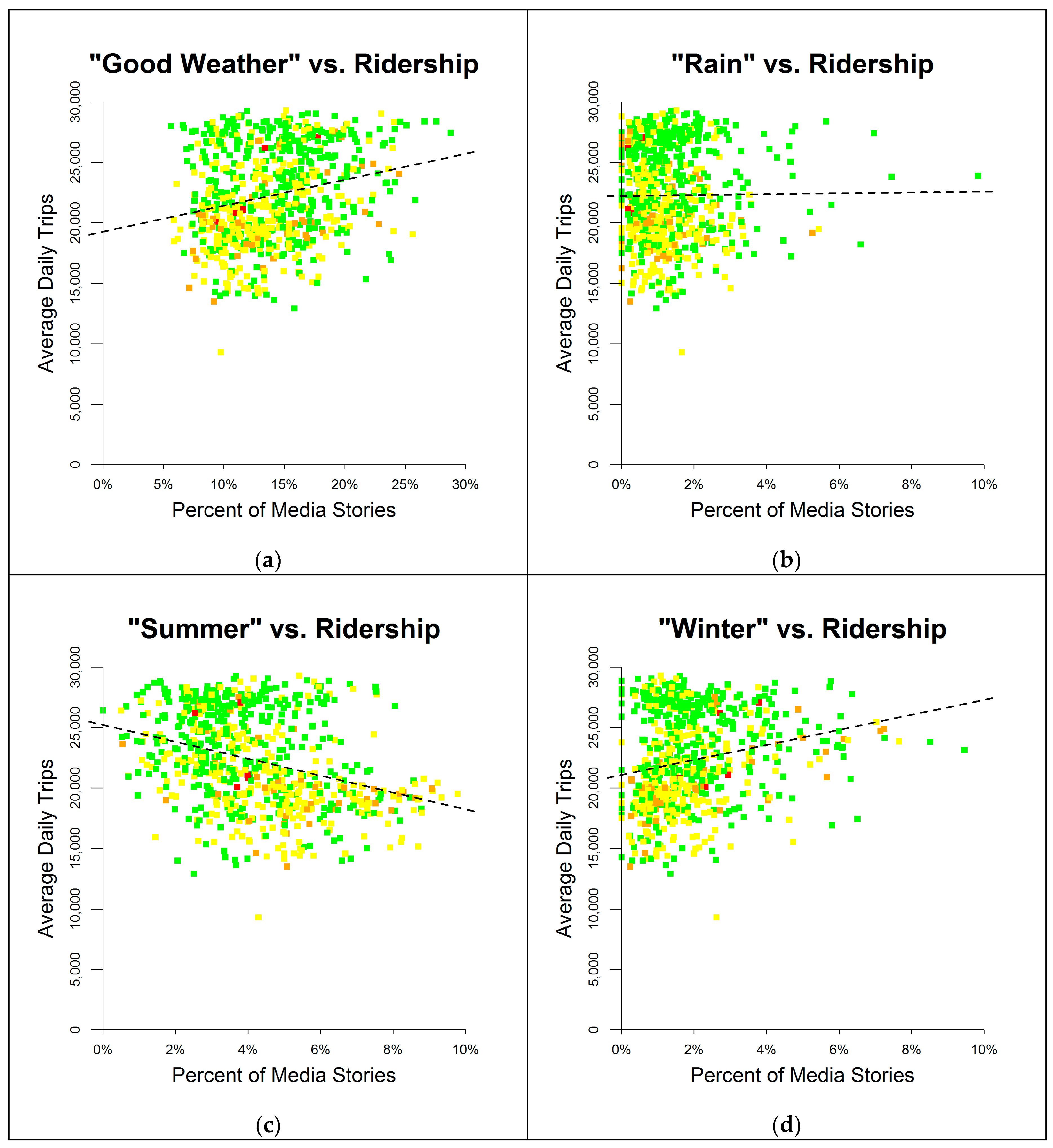
Figure 4.
Relationship between key term media count frequency and transit ridership for: (a) “cloudy” during the winter; (b) “cloudy” during the summer; (c) “cold” during the winter; and (d) “cold” during the summer. The color of the points illustrates the air quality index for each day. Note the different x-axis scales.

Table 1.
List of media influence search terms.
| Air Quality | Higher Temperature | Orange Air Day | Storm |
|---|---|---|---|
| Bad weather | Hot | Ozone | Summer |
| Cloudy | Hotter | Particulate matter | Sun |
| Cold | Hotter weather | PM2.5 | Sunny |
| Freezing | Inversion | Rain | Winter |
| Green air day | Low temperature | Red air day | Winter storm |
| Heat wave | Lower temperature | Snow | Yellow air day |
Table 2.
List of media sources used in this study.
| Media Type | Count | Description |
|---|---|---|
| Digital Native | 4 | Internet based source. Includes news sources that began on the internet such as organizational websites and blogs. Examples: CDC, Vox, Scroll |
| Print Native | 24 | Primarily print-based publication. Includes newspapers and magazines. Examples: New York Times, The Economist. |
| Video Broadcast | 12 | Primarily broadcast TV station media such as video transcriptions or closed captions. Examples: CNN, Fox News. |
Table 3.
Bus commute and non-commuter ridership trips comparison at different timescales and between air quality indices (G = Green, Y = Yellow, O = Orange, R = Red). For statistically significant results: * = p ≤ 0.05; ** = p ≤ 0.01; *** = p ≤ 0.001.
Table 3.
Bus commute and non-commuter ridership trips comparison at different timescales and between air quality indices (G = Green, Y = Yellow, O = Orange, R = Red). For statistically significant results: * = p ≤ 0.05; ** = p ≤ 0.01; *** = p ≤ 0.001.
| Bus Commute Trips | |||||||||||||||||
|---|---|---|---|---|---|---|---|---|---|---|---|---|---|---|---|---|---|
| AQ | Ann | Win | Spr | Sum | Fall | Jan | Feb | Mar | Apr | May | Jun | Jul | Aug | Sep | Oct | Nov | Dec |
| G-Y | 0.00 *** | 0.97 | 0.05 * | 0.41 | 1.00 | 0.20 | 0.72 | 0.89 | 0.90 | 0.69 | 0.11 | 0.87 | 0.31 | 0.39 | 0.01 * | 0.35 | 0.46 |
| G-O | 0.00 *** | 0.89 | NA | 0.61 | NA | 0.03 * | 0.06 | NA | NA | NA | 0.00 ** | 0.99 | 0.02 * | NA | NA | NA | NA |
| G-R | 0.59 | 0.57 | NA | NA | NA | NA | 0.28 | NA | NA | NA | NA | NA | NA | NA | NA | NA | NA |
| Y-O | 0.27 | 0.85 | NA | 0.64 | NA | 0.13 | 0.08 | NA | NA | NA | 0.08 | 0.94 | 0.07 | NA | NA | NA | NA |
| Y-R | 0.05 * | 0.49 | NA | NA | NA | NA | 0.29 | NA | NA | NA | NA | NA | NA | NA | NA | NA | NA |
| O-R | 0.01 * | 0.61 | NA | NA | NA | NA | 0.39 | NA | NA | NA | NA | NA | NA | NA | NA | NA | NA |
| Bus Non-Commute Trips | |||||||||||||||||
| AQ | Ann | Win | Spr | Sum | Fall | Jan | Feb | Mar | Apr | May | Jun | Jul | Aug | Sep | Oct | Nov | Dec |
| G-Y | 0.00 *** | 0.33 | 0.04 * | 0.66 | 0.94 | 0.14 | 0.39 | 0.90 | 0.39 | 0.98 | 0.21 | 0.45 | 0.55 | 0.09 | 0.02 * | 0.31 | 0.56 |
| G-O | 0.00 *** | 0.54 | NA | 0.54 | NA | 0.02 * | 0.04 * | NA | NA | NA | 0.02 * | 0.89 | 0.05 * | NA | NA | NA | NA |
| G-R | 0.65 | 0.47 | NA | NA | NA | NA | 0.09 | NA | NA | NA | NA | NA | NA | NA | NA | NA | NA |
| Y-O | 0.09 | 0.98 | NA | 0.78 | NA | 0.20 | 0.05 * | NA | NA | NA | 0.21 | 0.71 | 0.07 | NA | NA | NA | NA |
| Y-R | 0.05 * | 0.27 | NA | NA | NA | NA | 0.10 | NA | NA | NA | NA | NA | NA | NA | NA | NA | NA |
| O-R | 0.00 ** | 0.36 | NA | NA | NA | NA | 0.57 | NA | NA | NA | NA | NA | NA | NA | NA | NA | NA |
Table 4.
FrontRunner commute and non-commuter ridership trips comparison at different timescales and between air quality indices (G = Green, Y = Yellow, O = Orange, R = Red). For statistically significant results: * = p ≤ 0.05; ** = p ≤ 0.01; *** = p ≤ 0.001.
Table 4.
FrontRunner commute and non-commuter ridership trips comparison at different timescales and between air quality indices (G = Green, Y = Yellow, O = Orange, R = Red). For statistically significant results: * = p ≤ 0.05; ** = p ≤ 0.01; *** = p ≤ 0.001.
| Front Runner Commute Trips | |||||||||||||||||
|---|---|---|---|---|---|---|---|---|---|---|---|---|---|---|---|---|---|
| AQ | Ann | Win | Spr | Sum | Fall | Jan | Feb | Mar | Apr | May | Jun | Jul | Aug | Sep | Oct | Nov | Dec |
| G-Y | 0.00 *** | 0.74 | 0.00 *** | 0.34 | 0.50 | 0.19 | 0.82 | 0.48 | 0.68 | 0.24 | 0.06 | 0.66 | 0.27 | 0.80 | 0.02 * | 0.05 | 0.98 |
| G-O | 0.00 *** | 0.76 | NA | 0.38 | NA | 0.12 | 0.13 | NA | NA | NA | 0.01 * | 0.86 | 0.11 | NA | NA | NA | NA |
| G-R | 0.37 | 0.86 | NA | NA | NA | NA | 0.61 | NA | NA | NA | NA | NA | NA | NA | NA | NA | NA |
| Y-O | 0.86 | 0.88 | NA | 0.99 | NA | 0.50 | 0.12 | NA | NA | NA | 0.33 | 0.66 | 0.26 | NA | NA | NA | NA |
| Y-R | 0.74 | 0.73 | NA | NA | NA | NA | 0.75 | NA | NA | NA | NA | NA | NA | NA | NA | NA | NA |
| O-R | 0.71 | 0.69 | NA | NA | NA | NA | 0.37 | NA | NA | NA | NA | NA | NA | NA | NA | NA | NA |
| Front Runner Non-Commute Trips | |||||||||||||||||
| AQ | Ann | Win | Spr | Sum | Fall | Jan | Feb | Mar | Apr | May | Jun | Jul | Aug | Sep | Oct | Nov | Dec |
| G-Y | 0.00 *** | 0.77 | 0.00 *** | 0.12 | 0.40 | 0.31 | 0.95 | 0.60 | 0.63 | 0.08 | 0.01 ** | 0.54 | 0.10 | 0.59 | 0.00 ** | 0.11 | 0.78 |
| G-O | 0.00 *** | 0.96 | NA | 0.01 * | NA | 0.12 | 0.00 *** | NA | NA | NA | 0.01 * | 0.42 | 0.00 *** | NA | NA | NA | NA |
| G-R | 0.65 | 0.90 | NA | NA | NA | NA | 0.44 | NA | NA | NA | NA | NA | NA | NA | NA | NA | NA |
| Y-O | 0.48 | 0.89 | NA | 0.01 | NA | 0.32 | 0.10 | NA | NA | NA | 0.78 | 0.31 | 0.02 * | NA | NA | NA | NA |
| Y-R | 0.20 | 0.97 | NA | NA | NA | NA | 0.48 | NA | NA | NA | NA | NA | NA | NA | NA | NA | NA |
| O-R | 0.07 | 0.92 | NA | NA | NA | NA | 0.53 | NA | NA | NA | NA | NA | NA | NA | NA | NA | NA |
Table 5.
TRAX commute and non-commuter ridership trips comparison at different timescales and between air quality indices (G = Green, Y = Yellow, O = Orange, R = Red). For statistically significant results: * = p ≤ 0.05; ** = p ≤ 0.01; *** = p ≤ 0.001.
Table 5.
TRAX commute and non-commuter ridership trips comparison at different timescales and between air quality indices (G = Green, Y = Yellow, O = Orange, R = Red). For statistically significant results: * = p ≤ 0.05; ** = p ≤ 0.01; *** = p ≤ 0.001.
| TRAX Commute Trips | |||||||||||||||||
|---|---|---|---|---|---|---|---|---|---|---|---|---|---|---|---|---|---|
| AQ | Ann | Win | Spr | Sum | Fall | Jan | Feb | Mar | Apr | May | Jun | Jul | Aug | Sep | Oct | Nov | Dec |
| G-Y | 0.00 *** | 0.68 | 0.01 * | 0.07 | 0.83 | 0.12 | 0.76 | 0.34 | 0.67 | 0.29 | 0.06 | 0.66 | 0.04 * | 0.87 | 0.02 * | 0.15 | 0.85 |
| G-O | 0.00 *** | 0.87 | NA | 0.00 ** | NA | 0.05 | 0.32 | NA | NA | NA | 0.70 | 0.18 | 0.00 *** | NA | NA | NA | NA |
| G-R | 0.42 | 0.43 | NA | NA | NA | NA | 0.83 | NA | NA | NA | NA | NA | NA | NA | NA | NA | NA |
| Y-O | 0.15 | 0.92 | NA | 0.12 | NA | 0.43 | 0.20 | NA | NA | NA | 0.25 | 0.19 | 0.02 * | NA | NA | NA | NA |
| Y-R | 0.54 | 0.46 | NA | NA | NA | NA | 0.99 | NA | NA | NA | NA | NA | NA | NA | NA | NA | NA |
| O-R | 0.23 | 0.46 | NA | NA | NA | NA | 0.36 | NA | NA | NA | NA | NA | NA | NA | NA | NA | NA |
| TRAX Non-Commute Trips | |||||||||||||||||
| AQ | Ann | Win | Spr | Sum | Fall | Jan | Feb | Mar | Apr | May | Jun | Jul | Aug | Sep | Oct | Nov | Dec |
| G-Y | 0.00 *** | 0.27 | 0.01 * | 0.06 | 0.40 | 0.14 | 0.31 | 0.39 | 0.11 | 0.35 | 0.07 | 0.43 | 0.08 | 0.63 | 0.09 | 0.88 | 0.73 |
| G-O | 0.00 *** | 0.20 | NA | 0.00 ** | NA | 0.05 * | 0.68 | NA | NA | NA | 0.76 | 0.12 | 0.00 ** | NA | NA | NA | NA |
| G-R | 0.53 | 0.28 | NA | NA | NA | NA | 0.66 | NA | NA | NA | NA | NA | NA | NA | NA | NA | NA |
| Y-O | 0.03 * | 0.63 | NA | 0.04 * | NA | 0.46 | 0.31 | NA | NA | NA | 0.11 | 0.04 * | 0.04 * | NA | NA | NA | NA |
| Y-R | 0.37 | 0.56 | NA | NA | NA | NA | 0.74 | NA | NA | NA | NA | NA | NA | NA | NA | NA | NA |
| O-R | 0.06 | 0.78 | NA | NA | NA | NA | 0.41 | NA | NA | NA | NA | NA | NA | NA | NA | NA | NA |
© 2020 by the authors. Licensee MDPI, Basel, Switzerland. This article is an open access article distributed under the terms and conditions of the Creative Commons Attribution (CC BY) license (http://creativecommons.org/licenses/by/4.0/).
Share and Cite
MDPI and ACS Style
Mendoza, D.L.; Buchert, M.P.; Benney, T.M.; Lin, J.C. The Association of Media and Environmental Variables with Transit Ridership. Vehicles 2020, 2, 507-522. https://0-doi-org.brum.beds.ac.uk/10.3390/vehicles2030028
AMA Style
Mendoza DL, Buchert MP, Benney TM, Lin JC. The Association of Media and Environmental Variables with Transit Ridership. Vehicles. 2020; 2(3):507-522. https://0-doi-org.brum.beds.ac.uk/10.3390/vehicles2030028
Chicago/Turabian StyleMendoza, Daniel L., Martin P. Buchert, Tabitha M. Benney, and John C. Lin. 2020. "The Association of Media and Environmental Variables with Transit Ridership" Vehicles 2, no. 3: 507-522. https://0-doi-org.brum.beds.ac.uk/10.3390/vehicles2030028