Article

Statistical Validation of Energy Efficiency Improvements through Analysis of Experimental Field Data: A Guide to Good Practice

by
Konstantinos Demestichas
* and
Evgenia Adamopoulou
School of Electrical and Computer Engineering, Institute of Communication and Computer Systems, National Technical University of Athens, Iroon Polytechneiou 9, Zografou, 15773 Athens, Greece
*
Author to whom correspondence should be addressed.
Submission received: 10 August 2020 / Revised: 28 August 2020 / Accepted: 31 August 2020 / Published: 7 September 2020

Abstract

:
Often in the area of road transport solutions and intelligent transport systems, two or more alternative solutions or methods compete in terms of energy gains, time efficiency, or other aspects. Measurements collected from field trials are used to make a comparative assessment but are usually limited because of resource constraints. The present paper describes how statistical inference techniques can be used in a systematic way, in order to validate the superior performance of one method over the other. We adopt such an approach to study the performance of two alternative routing methods in terms of achievable energy savings, although the same methodology can be widely applied to other use cases as well. We specifically employ and describe three different techniques to achieve the intended comparison, namely paired sample tests, statistical testing of mean value in a normal population, and two-sample tests in normal populations with unknown yet equal variances. We reach conclusions on whether claims of outperformance of one routing method over the other can be supported by our collected experimental data and to what extent.

1. Introduction

This paper concentrates on revealing and explaining practical and systematic ways in which the results of different methods designed and applied in the area of intelligent transport systems (ITS) can be effectively compared against each other. The motivation behind this study resides in the claims often found in research articles (e.g., [1,2]) and technical projects (e.g., [3,4,5,6]) that a newly proposed method (for instance, on topics relevant to driving performance, efficient routing, traffic prediction, vehicular communication) leads to a significant improvement in terms of energy efficiency (e.g., energy savings in the order of 10–20% over the state-of-the-art). Such a claim is often dealt with skepticism from the relevant evaluators, because of the usually limited-in-size measurement samples. Moreover, the validation of such claim from the researchers’ side is often not dealt with the proper care. For this reason, the validation of a new method is frequently limited to qualitative criteria and the quantification of the results is usually avoided.

1.1. Aim and Research Questions

Considering the above, the focal point of this paper is to investigate and describe ways of validating if and to what extent a method over-performs compared to a conventional, alternative one. In this context, we employ and apply the hypothesis-testing method of the statistical inference science. In particular, to properly exemplify our approach, we discuss on ways of evaluating two different routing methods, i.e., methods of identifying the optimal route from an origin point to a destination point inside the road network. In detail, our goal is to investigate the validity of arguments such as the following:
  • Does Method A provide better results than Method B according to a certain routing criterion? As such criterion, the vehicle’s energy consumption is considered in our use case. Thus, in other words, we would like to study whether the average energy consumption of a vehicle following the same routing method A is statistically lower than the consumption of the same vehicle following routing method B.
  • Is Method A better at a γ% percentage compared to Method B, on the basis of the adopted routing criterion? In other words, we would like to examine whether the average energy savings percentage of a vehicle following routing method A is at least γ% compared to the energy consumption of the same vehicle following routing method B.
In order to provide convincing answers to the above posed questions, a proper statistical analysis of the available experimental data should be performed. In particular, we employ, establish and describe the process of hypothesis testing of the statistical inference for drawing relevant conclusions. To the best of the authors’ knowledge, it is the first time that such a systematic and practical approach is explained in the literature for transport-related use cases. It is also worth noting that, despite the fact that our study concentrates on the comparison and validation of routing methods, based on real experimental data, the same techniques can be adapted and followed in a wide range of transport-related application domains, such as driving efficiency, driver profiling, traffic prediction and optimization, logistics, vehicular communication, and others.

1.2. Related Work

To substantiate the importance of this issue, we examine papers from the literature related to energy, fuel, or emissions improvements brought by novel methods in the fields of eco-driving and green routing.
For instance, the work in [7] evaluated, among other aspects, the CO2 benefits of eco-driving for various degrees of penetration rates (from 25% up to 100%) and three levels of traffic congestion. It was found that, under free flow traffic, the savings can reach 15% and in normal traffic 10%. In contrast, in cases of congested traffic, it was found that the presence of eco-drivers could increase the overall CO2 emissions. The work in [8] proposed an eco-approach and departure application which uses information coming from fixed-time traffic signals to guide a driver through the intersection in an environmentally friendly way. The authors report a reduction in emissions in the range of 11–30% when the initial speed is low (up to 30 mph) and a smaller reduction in-between 3.3% and 6.2%, depending on the type of pollutants, for higher initial speeds. The study in [9] evaluated the environmental benefits of time-dependent green routing in the greater Buffalo-Niagara region of the U.S., using a combination of two simulation models. Results show that the percent reduction was 12.76% for trucks (vs. 12.63% for passenger cars) when attempting to minimize CO emissions, and 10.22% (vs. 10.37% for passenger cars) when minimizing NOx. The study in [10] assessed the efficiency of eco-driving as a means for reducing the fuel consumption of freight transport. A large field test was carried out in the Chinese province of Jiangsu, showing savings of fuel up to 5.5% for high-duty vehicles, but not substantial benefits for light commercial vehicles. None of these papers reports the use of a statistical validation approach for their findings.
The work in [11] provides a comprehensive overview of many solutions for the improvement of green-house gas (GHG) emissions of road freight transport. Specifically, the authors in [11] review 58 relevant solutions and classify them into four classes, according to the percentage of CO2 equivalent (CO2e) savings that they can achieve (Class I: 0–6%; Class II: 6–11%; Class III: 11–16%; Class IV: >16%). In the context of the present paper, we select and examine four of these solutions in terms of the approach that they have followed to validate the percentage of CO2e savings. The selection was random, but we made sure to cover all different classes and to select papers that spanned different years and that contained case studies conducted in various geographic regions.
In this framework, the study in [12] (Class I) presented a methodology based on a Geographic Information System (GIS) model developed in order to improve fuel and CO2 efficiency of a Greek municipality’s waste collection and transport system, via the reallocation of waste collection bins and the optimization of vehicle routing in terms of distance and time travelled. Using a simulation model coupled with a field study, the authors show that the routing optimization results in a 5.5–12.5% reduction in the distance travelled by the waste collection vehicle, in comparison to the empirical route. The validation approach is not based on statistical inference and it is not clear whether the reported results constitute average values.
The research approach presented in [13] (Class II) adopted a probabilistic model for vehicle routing and scheduling problems with time windows that was finetuned and applied using a test vehicle in the area of South Osaka, Japan. The authors reported average CO2 savings of 7.6%, as well as similar reductions in local pollutants, compared to the previous routing solution. Although the authors report not just the average values but also the standard deviations of their measurements, yet they do not proceed in a systematic statistical validation.
The work in [14] (Class III) employed the vehicle specific power concept and used second-by-second vehicle dynamics to extract the emissions on various route alternatives, based on car-floating data collected from various regions in Portugal. Results show that choosing eco-friendly routes can lead to significant savings in CO2 (up to 25%) and other types of emissions. Descriptive statistics and boxplots are provided for the collected measurements in various routes under investigation, however reductions in emissions are presented in the form of percentages compared to the worst alternative route available, without elaboration on the type of statistical validation employed.
The study in [15] (Class IV) proposed an environmentally conscious optimization model of a supply chain network, based on integer non-linear programming, with an expanded objective function that takes not only transportation costs into account, but also environmental parameters, such as GHG emissions, fuel consumption, noise, and others. The paper studies various solutions related to the planning of changes in suppliers’ or manufacturers’ capacity in a simulated supply chain network. The impact of these planning decisions is reported in terms of percentages (e.g., in the environmental, transportation, and overall costs) against the baseline scenario, without further elaboration on the statistical significance of these results.
Beyond the aforementioned four papers, there are also other interesting relevant studies that we have found and reviewed. For instance, the study in [16] (corresponding to Class II) conducts a thorough assessment of the impact of green navigation systems in a city’s traffic flows, combining a macroscopic traffic model with a macroscopic emissions model and a GIS. Results show up to 10.4% reductions in CO2 and up to 13.8% in NOx in congested traffic conditions for a 90% penetration of green drivers, but also that the overall population’s exposure to NOx increases up to 20.2%. Similarly, the eco-routing study in [17] in Lund (corresponding to Class I), Sweden, showed that in 46% of journeys (in a sample of 109 journeys), drivers do not choose the most fuel-efficient route. It also showed that green routing can lead to a mean saving of 4.0% in fuel. Despite the thoroughness of these reports, details on the approach followed for the statistical validation of the corresponding results were not provided.
The examples presented above are only a few from a range of studies related to improvements in energy, fuel, and emissions in road transport, which often neglect to present the validation of their results through statistical inference. There might be several reasons for this, e.g., sometimes authors might choose to place more emphasis on the description of their scientific or technological solution rather than on the validation of their results. In other cases, researchers might wish to keep the presentation of results as simple as possible, in order to be able to communicate them more easily to the uninitiated reader. In others, the researchers might not be familiar with the statistical testing process that they have to follow in order to validate their claim, and this reports only average and best-case results as well as standard deviations.
On the other hand, there are also studies in which the authors place adequate emphasis on validation based on statistical inference, even if the corresponding descriptions are somewhat limited. The approaches followed and presented in [18,19,20,21] are the most relevant to our work presented herein.
In [18], the authors proposed a novel eco-routing technique using vehicle-to-infrastructure communication, according to which a vehicles registers its fuel consumption when it transverses a road link and then transmits it to a traffic management center, so that next vehicles can exploit this information. Using simulation results and the analysis of variance, the authors show that the effect of the packet delay and packet loss are not statistically significant on the eco-routing system performance. In [19], the authors evaluated the impact of car dashboards on real-world eco-driving behavior. Particularly, the study assessed the effect of numeric and symbolic eco-driving feedback against a control group, by means of field trials conducted in Switzerland. Using a series of regression analyses, results showed that only the symbolic feedback design led to significant reductions of 2–3% in fuel consumption. In [20], the authors employ a smartphone application as a means of eco-feedback and assess its impact on fuel efficiency. Using a systematic statistical validation approach based on paired sample tests, the authors demonstrate an improvement of 3.23% in the overall fuel efficiency. In [21], the authors proposed a dynamic eco-driving approach in an arterial corridor with traffic signals, based on velocity planning algorithms which can achieve approximately 10–15% fuel economy improvement.
In summary, the former study [18] uses simulation results (instead of field data), the second one [19] focuses on regression analysis and the use of a control group, the third one [20] employs paired sample tests for validating fuel efficiency, although it does not elaborate on what approach can be followed in cases where paired sample tests are not possible, whereas the fourth one [21] involves a statistical t-test, although it does not reveal sufficient details (such as the null hypothesis). Thus, these four papers, which seem to have a strong methodological component, all feature some limitations and/or differences with the type of analysis proposed herein.
The remainder of this paper is organized as follows: Section 2 provides the background relevant to the methodology employed for the statistical validation. Section 3 describes the experimental data and elaborates on three different approaches of comparative assessment regarding the efficiency of two competing routing methods. Also, the same section draws practical guidelines for the applicability and limitations of the three approaches. Section 4 draws additional useful conclusions.
2. Methodology-Statistical Hypothesis Testing Process

The following paragraphs describe an overview of the basic steps of the statistical hypothesis testing process, in order to provide the main theoretic background for the proposed methodology [22,23]. Hence, the objective of statistical control is often to evaluate a hypothesis regarding the values of one or more parameters of a population [24]. In a statistical hypothesis, all parameters of a distribution can be determined partially or completely. A statistical hypothesis in which there is only one unknown population parameter is called a simple hypothesis, whereas in case there are two or more unknown parameters, the hypothesis is referred to as a composite hypothesis [25]. Some indicative examples of simple and composite hypotheses in the case of a normal population (when the only unknown parameters are the mean value μ and the variance σ2 of the population) are presented below:
i.
μ = μ0, σ2 = ω0 (simple hypothesis)
ii.
μ = μ0, σ2 > ω0 (composite hypothesis)
iii.
μ = μ0 (simple hypothesis)
The four primary components of hypothesis testing are the null hypothesis, the alternative hypothesis, the critical region, and the test statistic. The statistical hypothesis under consideration is called null hypothesis and is often denoted as H0. For each null hypothesis, a suitable alternative hypothesis is also determined, denoted as HA.
The alternative hypothesis, for example, for the null hypothesis H0: μ = μ0 can take one of the following forms:
i.
HA: μ > μ0 (right-tailed, directional)
ii.
HA: μ < μ0 (left-tailed, directional)
iii.
HA: μμ0 (two-tailed, non-directional)
The form of the selected alternative hypothesis is determined by the conclusion that is desired to be drawn in case of rejection of the null hypothesis H0. The definition of the form of the alternative hypothesis affects the positioning of the so-called critical region.
After determining the null and the alternative hypothesis, the observed value of the test statistic is calculated, a process enabling the approval or rejection of the null hypothesis. In order for this decision to be taken, the sample space is divided into two mutually exclusive and complementary areas: the critical region and its complementary region. If the observed value of the test statistic resides inside the critical region, then the null hypothesis H0 is rejected. In the opposite case, when the observed value of the test statistic resides outside of the critical region, the null hypothesis H0 is accepted.
At this point, it should be highlighted that the terms acceptance and rejection should not be considered with their literal meaning; for example, acceptance of the null hypothesis does not necessarily mean that the latter is true. It just means that, based on the experimental or observation data, there is no reason to believe otherwise. In the same sense, rejection of the null hypothesis does not necessarily mean that it is false, but rather that the experimental data do not substantiate its approval as true.
As known, in order to reach conclusions on the attributes or characteristics of a population a sample of and not the entire population is studied. Thus, for any decision rule applied, an error at the acceptance or rejection of the hypothesis exists. The four possible cases are depicted in Table 1.
Table 1 indicates that two error types may exist during the decision process:
  • Type I error: Rejection of hypothesis H0 while the latter is true
  • Type II error: Acceptance (or no rejection) of H0 when the latter is false
The corresponding error probabilities are expressed as:
  • Probability of type I error = P (rejection of H0 | H0 is true) = α
  • Probability of type II error = P (acceptance of H0 | HA is true) = β
Using quality control terms, type I error corresponds to the case of a batch being rejected despite of being good and, thus, is referred to as producer’s risk, while type II error is related to the case of a faulty batch being accepted and is referred to as consumer’s risk.
Significance level. The probability of Type I error (α) is also referred to as level of significance and reflects the size of the critical region.
Power function. The probability of rejecting H0 when HA is true is called power function. It states that:
Power function = P (rejection of H0| HA is true) = 1 − P (acceptance of H0 | HA is true) = 1 − β
During the statistical hypothesis testing process, the minimization of the probabilities of both error types is ideally desired. Unfortunately, for a sample of given size n, these two probabilities cannot be controlled simultaneously. This occurs because any decrease of one error type leads to the increase of the other. For example, if a critical region where type I error is zero exists, then this means that hypothesis H0 will always be accepted and, therefore, the probability of Type II error will be equal to 1. Thus, it is necessary to maintain the probability of one type of error at a fixed level and select the critical regions, so that the probability of the other type of error is minimized. Since Type I error is considered to be more important than type II error, a value for the Type I error probability, a, is selected and the probability of Type II error, β, is minimized by maximizing the power function.
To sum up, the steps performed during a statistical hypothesis testing process are:
  • Identification of the population distribution and determination of the parameters of interest (e.g., mean value), which will be the subject of hypothesis testing. Identification of the null hypothesis H0 as well as of the form of the alternative hypothesis HA.
  • Selection of a suitable test statistic.
  • Identification of the critical region.
  • Calculation of the observed value of the test statistic.
Acceptance or rejection of the null hypothesis, depending on whether the observed value of the test statistic resides inside or outside the critical region, respectively.

3. Experimental Process and Results

3.1. Description of the Experiment and the Collected Dataset

In the framework of our study, let us assume that our research engineers declare that routing Method A provides better results than routing Method B regarding the energy consumption of a test electric vehicle. In order for this claim to be either verified or proven inaccurate, an experiment comprising 30 field tests is performed. In detail, 30 pairs of origin-destination points inside a trial site (i.e., specific geographic area) are selected in a random manner.
In the specific dataset, the distance of each destination point from the corresponding origin point ranges from 2 km to 4 km inside the road network. For each pair of origin-destination points, two routes are calculated and then travelled: the route suggested by Method A and the route suggested by Method B. For each of the 30 trials (i.e., for each pair of origin-destination points), the two routes are travelled under the same external conditions, i.e., with the same electric vehicle and driver, inside the same time frame (e.g., 12:00–14:00), at the same day of the week and the same month, with similar initial battery levels and under the same weather conditions. It should be noted that external factors may change from one trial to another, but not between routes of Type A and Type B of the same trial. In case that the external conditions change substantially, within the same trial, when driving the Type-A and Type-B routes, the measurements of the specific trial are discarded.
Furthermore, before each test, the method (i.e., Type A or Type B) to be tested first is selected in a completely random way (by tossing a coin). Moreover, in each trial, the driver is kept unaware of whether the route being travelled is of Type A or Type B, so as to avoid any bias in the results due to systematic changes in driver behavior.
In this study, Method A is based on the use of neural networks [26,27,28] for the estimation of the energy consumption of alternative routes to the desired destination. Once the energy cost of every road segment toward the selected destination is estimated by the neural networks (a properly trained neural network is used for each segment of the road network), the route, i.e., the sequence of adjacent road segments, that is expected to lead to the lowest energy consumption is computed and suggested to the driver.
On the other hand, Method B relies on the use of a currently commercially available routing software, whose routing algorithm selects the fastest route from the origin to the destination point according to the denoted speed limits but also based on historical and car-floating data of travelling times through the urban road segments.
Table 2 summarizes an excerpt of the test results. As can be observed, the results for both routes travelled are recorded in each trial. In detail, the route length (LENGTH in meters), the consumed energy (ENERGY in Watt-hours), the time travelled (TIME in seconds), as well as the number of road segments (LINKS) are recorded for each type of route (Type A or Type B).
Subsequently, in order to compare the energy consumption, the following ratio is used:
ξ i = e A i e B i e B i ,     w h e r e   i = 1 ,   2 ,   . ,   30
and the result is stored inside the “Energy (Ratio)” table column, with e A i and e Β i representing the recorded energy consumption values for the Type A and the Type B route, respectively, at the end of the ith trial.
In order to verify or disprove claims such as the ones presented in the Introduction, regarding the comparative performance of the two routing methods, A and B, we proceed to formulate a suitable statistical hypothesis testing process, taking advantage of the collected experimental data.

3.2. Paired Sample Tests

The grouping of available observations into pairs is a method aimed at reducing the usually large variance that exists in the effects of two so-called “treatments” (candidate solutions). Under the assumption that a suitable external factor is selected for implementing the grouping into pairs, the usual methods of statistical inference (hypothesis testing and confidence intervals) are rendered more efficient for detecting actual differences in the average influences of different treatments [24].
Based on the experimental results of Table 2, we consider n = 30 random pairs of energy consumption observations ( E A i ,   E B i ) in n respective combinations of the external factors’ values (external conditions), where in each pair the observation E A i corresponds to the first “treatment” (Method A) of the ith trial and the observation E B i corresponds to the second “treatment” (Method B) of the ith trial, respectively. The following assumptions are made for these random pairs:
  • Concerning the ( E A i ,   E B i ) pairs: For each i (where i = 1 ,   2 ,   ,   n ), the random pair ( E A i ,   E B i ) has a two-dimensional normal distribution with parameters μ E A i ,   μ E Β i ,   σ E A i ,   σ E Β i ,   ρ E A i , E Β i such that:
    μ Ε A i = μ + μ D ,   μ Ε B i = μ σ Ε A i = σ Ε A ,   σ Β A i = σ Ε Β ρ E A i , E Β i =   ρ E A , E Β
    and that the random pairs ( E A 1 ,   E B 1 ) ,   ( E A 2 ,   E B 2 ) ,   ,   ( E A n ,   E B n ) are random vectors independent from one another.
  • Concerning the differences D i =   E A i E B i : The differences D 1 ,   D 2 ,   ,   D n   , where:
    D i = E A i E B i ,   where   i = 1 ,   2 ,   ,   n
    comprise a random sample out of a normal population with mean value μ D . Thus, we assume that the random variables D 1 ,   D 2 ,   ,   D n constitute a random sample of a normal population with mean value equal to the difference μ D of the average values of each pair’s observations [24].
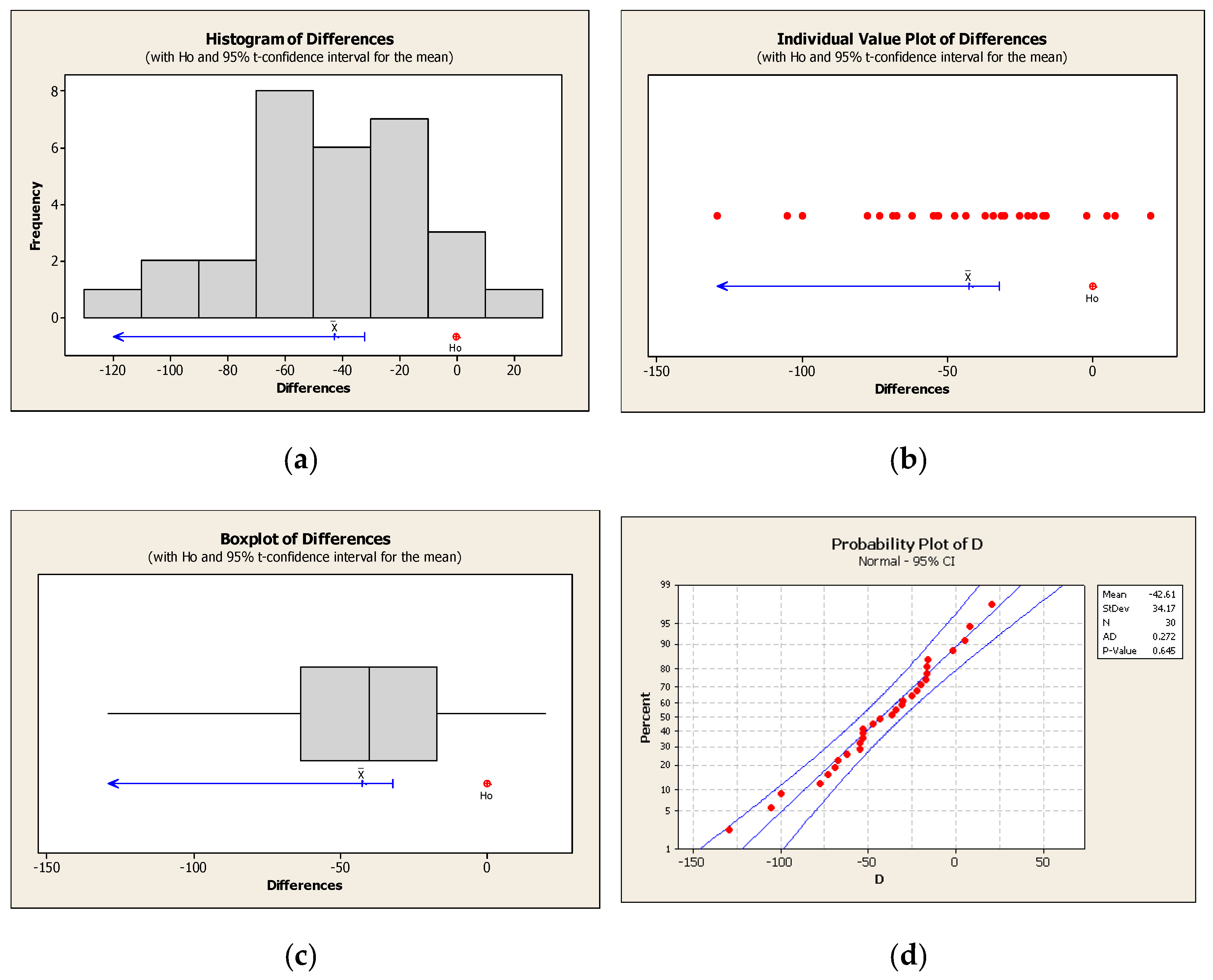
Figure 1 provides a through description of the measured D i differences of the paired samples by means of a histogram, an individual value plot and a boxplot. Part (d) of Figure 1 contains a normal probability plot that confirms that the measured differences follow a normal distribution (since the data points fall within the area defined by the adjustment to the normal model).
Consequently, the steps of the statistical test process are described below:
Step 1: In order to investigate whether the average energy consumption of Method A is lower than the energy consumption of Method B, we must check the following null hypothesis:
H 0 : μ D = 0
This null hypothesis is tested against the alternative hypothesis:
H A : μ D < 0
In case our statistical test supports the acceptance of the null hypothesis, then there will be strong indications that the average energy consumption through the application of Method A is equal to or greater than the energy consumption through the application of Method B. In other words, acceptance of the null hypothesis suggests that Method A does not have better results regarding the energy consumption compared to Method B. On the other hand, rejection of the null hypothesis (and consequent acceptance of the alternative hypothesis) implies that Method A provides indeed better results (i.e., lower energy consumption on average).
Step 2: The test statistic that should be used is:
T = D ¯ δ 0 S D / n
where D ¯ is the sample mean value and S D the sample standard deviation of the D i values, while the critical region is the following:
C = { t : t < t a , n 1 }
Setting α = 0.05 as the significance level and with n = 30, we have:
C = { t : t < t 0.05 , 29 } = { t : t < 1.699 }
It should be highlighted herein that the normal practice is to work with only one significance level (fixed in advance). By convention, typical values for α used in the literature are: 0.10, 0.05, or 0.01 [29]. In this paper, we report and discuss results when working with any of these typical levels.
Step 3: The observed value of the test statistic is:
t = d ¯ δ 0 s D / n
where d ¯ = 42.61 , δ 0 = 0 , s D = 34.171 , n = 30 and thus:
t = 6.830
Step 4: The observed value of the statistical test function falls inside the critical region, thus, we reject the null hypothesis H 0 , since:
t = 6.830 <   1.699
Step 5: Rejection of H 0 suggests that we have adequate evidence that Method A achieves lower average energy consumption than Method B or, in other words, that by adopting Method A the vehicle saves energy.
From the results summarized in Table 3, we confirm that the observed value of the test statistic is the one calculated in Step 3, and the observed significance level is p = 0.000 (i.e., with accuracy of three decimal places) which means that p < α for all typical values of the significance level α (typically, 0.10, 0.05, and 0.01). Hence, the null hypothesis is rejected at all three levels of significance and the alternative hypothesis is accepted, resulting in the conclusion that Method A indeed achieves lower energy consumption compared to Method B.
Expanding our conclusions, we can observe that, since the 95% confidence level for the average difference is equal to −32.01, as depicted in Table 3, there is sufficient evidence at the 5% significance level that Method A achieves average energy savings greater than 32 Wh compared to Method B in urban routes of 2–4 km length.

3.3. Statistical Testing of the Mean Value in a Normal Population (with Unknown Variance)

By performing the statistical analysis of the previous section (Section 3.2), we succeeded in answering two types of questions: (1) whether Method A achieves-on average-better results than Method B and (2) whether Method A achieves, on average, energy savings greater than δ0 energy units (Wh) in 2–4 km urban routes. Going one step further, we would like to investigate whether the average energy saving achieved by Method A over Method B is of the order of γ% (e.g., γ = −10%) or better. In other words, we would like to quantify even further the benefits of adopting Method A over Method B and verify or disprove a claim that Method A leads to average energy savings in the order of γ% or better.
To this end, we calculate through Equation (2) the ratios ξ i ,   w h e r e   i = 1 ,   2 ,   . ,   30 . The values of ξ i represent the ratio of the energy difference between the Type A route and the Type B route as a percentage of the energy consumed in the Type B route, for the ith trial.
Before proceeding with the selection of the most appropriate statistical hypothesis test, it is necessary to confirm our “intuition” about the normality of the population. The corresponding graphic normality test is depicted in Figure 2. Figure 2 suggests that our data conform to the normal distribution with average value μ ^ Ξ = Ξ ¯ = 0.1182 and standard deviation equal to σ ^ Ξ = s Ξ = 0.08369 . This conclusion is drawn [24] not only because all points in the graph fall within the area defined by the adjustment to the normal model but also because the observed significance level of the Anderson-Darling (AD) criterion is greater than all typical significance levels. In particular, p = 0.486 > α for α equal to 0.10, 0.05, and 0.01. The AD criterion is used to test if a sample of data belong to a population following a particular distribution [30] (in this case, the normal distribution). It is based on the Kolmogorov-Smirnov (K-S) test but uses tables of critical values for the distribution under consideration.
Consequently, we may proceed in testing the mean value of the normal population with unknown variance. In this case, the most suitable test statistic is:
T = Ξ ¯ μ Ξ s Ξ / n
Accordingly, we carry out the following testing procedure. The null hypothesis to be tested is:
H 0 : μ Ξ = γ
where μ Ξ is the average value of the ratio D i / E B i and γ < 0. The null hypothesis is tested against the alternative:
H A : μ Ξ > γ
In case the null hypothesis is accepted, there will be strong evidence that the average difference of Type A and Type B energy consumption is equal to or better than γ% compared to the average Type B consumption. In other words, acceptance of the null hypothesis means that Method A presents energy savings equal to or better than γ% compared to Method B. For instance, if γ = −10% or γ = −0.10, then accepting the null hypothesis suggests that there are average energy savings of 10% or greater if Method A is selected over Method B. If γ is lower, then the benefit obtained from using Method A is higher.
By executing the corresponding statistical test, we get the results depicted in Table 4. As can be seen, the observed significance level is p = 0.878 which means that p > α for all typical values of the significance level α (0.10, 0.05, and 0.01). Hence, for all typical significance levels, the null hypothesis is accepted and the alternative is rejected, resulting in the conclusion that Method A indeed achieves average energy savings equal to or better than 10% compared to Method B.
Expanding our conclusions, we observe that the 95% confidence interval for the mean value μ Ξ has a lower bound at −0.1442. This means that there is strong evidence at the 5% level of significance that Method A achieves average energy savings 14% or better compared to Method B. On the other hand, there is no sufficient evidence at this level of significance that the average energy savings are greater than 15% when Method A is selected.

3.4. Statistical Testing of the Difference of the Mean Values of Two Populations with Independent Samples

There are cases where the paired-wise comparison employed in Section 3.2 cannot be applied, because the conditions used for the data collection between Method A and Method B differ substantially. For instance, when it cannot be ensured that the Type-A route and the Type-B route in each trial can be travelled in the same time window, with the same driver or in the same weather conditions. In such cases, in which the field trials are designed in such a way so that the two sets of experimental data are collected (run by run) for the same origin and destination points but in different contexts (external conditions), and are thus independent, then the paired sample methodology of Section 3.2 cannot be applied, but an alternative statistical validation approach exists.
In this light, hereinafter we assume that we have two independent samples: Sample A regarding the energy consumption when using routing Method A, and Sample B regarding the energy consumption when using routing Method B. The test statistic that should be used in this case is:
T = E A ¯ E B ¯ δ 0 S p 1 n A + 1 n B
which follows the t-distribution with nA + nB 2 degrees of freedom, when hypothesis H0 is true. In Equation (13), E A ¯ and E B ¯ represent the average energy consumption values of the two samples A and B, respectively, whereas nA and nB represent the sizes of the two samples, respectively. In addition, δ 0 represents the difference between the mean values of populations A and B (see also Table 5).
The metric Sp is the square root of the weighted sampled variance, which is given by:
S p 2 = ( n 1 1 ) S A 2 + ( n 2 1 ) S B 2 n A + n B 2
where S A and S B denote the standard deviations for the two samples. The critical region in this case is given in Table 5.
The statistical testing described above is used in practice when the sample size is small and the distributions of the two populations do not differ significantly from the normal distribution. Furthermore, this testing is usually performed after first conducting an F testing for the ratio of the variances of the two populations, and after ensuring that the null hypothesis that this ratio is equal to 1 has not been rejected. However, it is also applied in case where the hypothesis of equality of the two variances has been rejected, but the samples are of equal size.
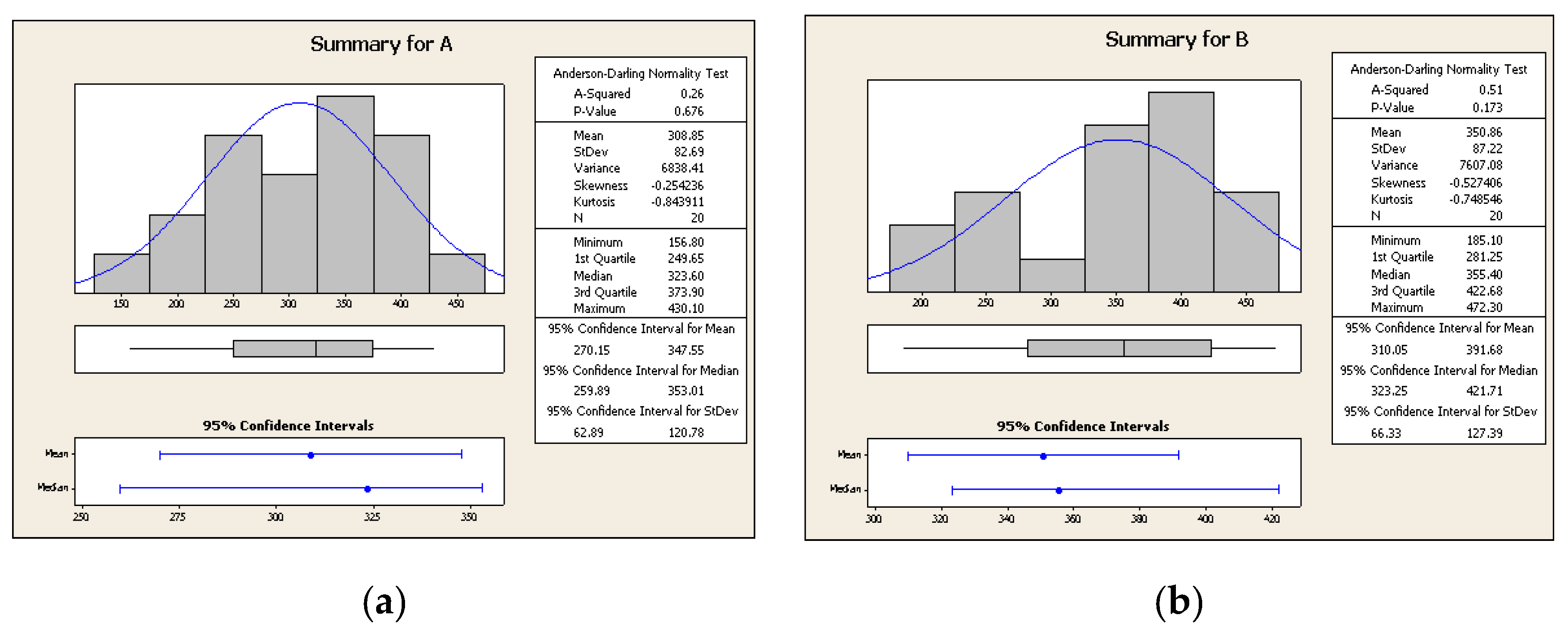
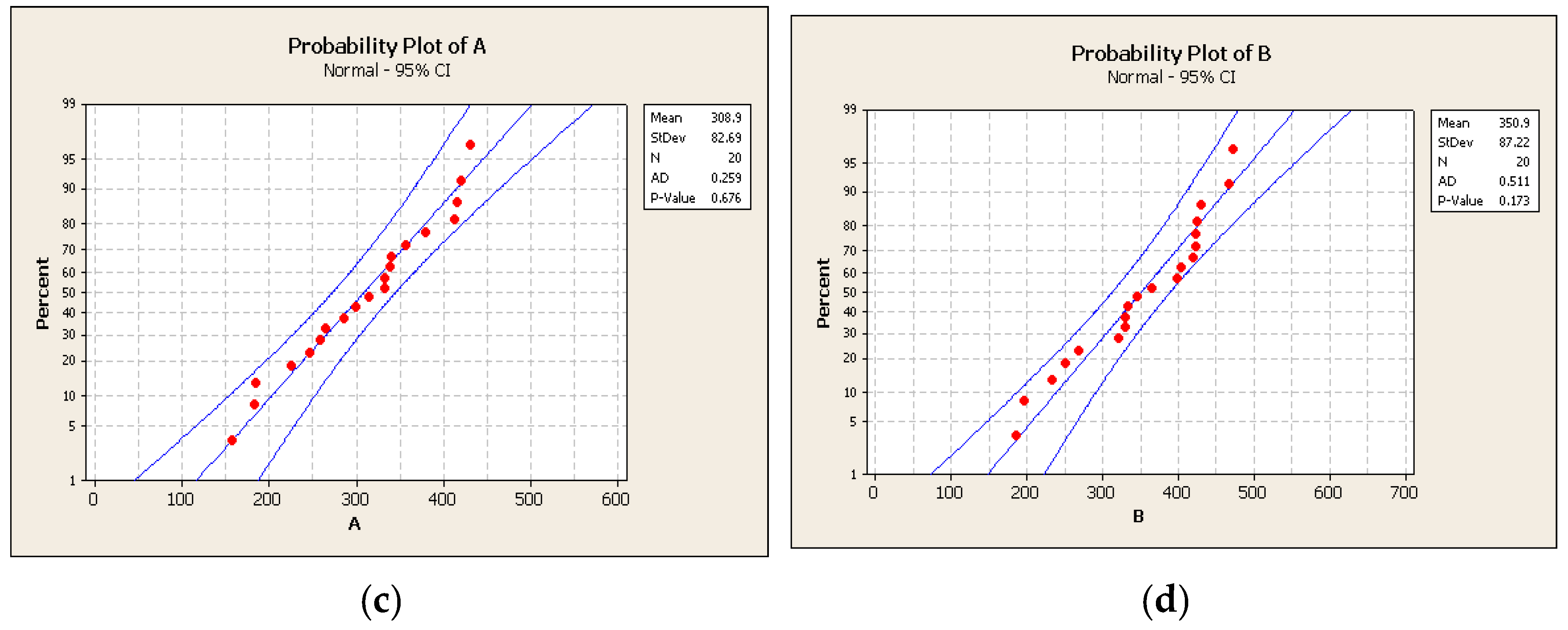
Hereafter, we further elaborate on how to apply this method and its respective limitations. As aforementioned, this time we have collected two independent sets of field measurements, i.e., two independent samples, which are different from the ones used in the previous, paired tests of Section 3.2. These two independent samples, A and B, are of equal size n = 20, and their descriptive summary is given in Figure 3a,b, respectively. We first test whether the collected data follow the normal distribution, as illustrated in Figure 3c,d. The test for normality is necessary because the sample sizes are small (i.e., n < 30).
Based on Figure 3, we observe that, for both populations, data conform to the normal distribution, since all points in the two graphs fall within the area defined by the adjustment to the normal model, and also because the observed significance level of the Anderson-Darling (AD) criterion is greater than the typically used significance levels (i.e., p > α for α equal to 0.10, 0.05, and 0.01). In case the populations from which the samples are taken do not have a normal probability distribution (e.g., supposedly the population from which sample B is drawn follows the skewed distribution), then it is not valid to follow the method suggested in this section. In such case, it is best to enlarge the samples (i.e., n 30 ), which allows the Central Limit Theorem to be applicable and a simple Z-test [31] can be used [32].
As explained, since the two sample sizes are equal, we may directly proceed into using the method defined, but it is better first to test whether the two unknown variances can be assumed as equal. For this, we use the F-test, as depicted in Table 6, to test the hypothesis of the two variances being equal against the alternative of not being equal, i.e.,:
H 0 :   σ A 2 σ Β 2 = 1     v s .     H A :   σ A 2 σ Β 2 1
From the results of the F-test, we deduce that there are strong indications to accept the null hypothesis, since the observed significance level p is higher than the typical significance levels (i.e., p > α for α equal to 0.10, 0.05, and 0.01).
Subsequently, we carry out the main testing procedure, by testing the following null hypothesis:
H 0 : μ A μ Β = 0
where μ A and μ B are the mean values of populations A and B, respectively, whereas γ < 0. The null hypothesis is tested against the alternative:
H A : μ A μ Β < 0
In case the null hypothesis is accepted, there will be strong evidence that the average difference of Type A and Type B consumptions is zero. In other words, acceptance of the null hypothesis means that there is no proof that Method A presents energy savings compared to Method B, whereas acceptance of the alternative hypothesis means that Method A leads to lower energy consumption on average compared to Method B.
By executing the corresponding statistical test, we get the results depicted in Table 7. As can be seen, the observed significance level is p = 0.063 which means that p > α for α = 0.01 and α = 0.05. Hence, at these two typical significance levels, the null hypothesis is accepted and the alternative is rejected, resulting in the conclusion that there is no substantial evidence that Method A achieves better average energy savings against Method B. We also observe that the 95% confidence interval for the difference μ A μ Β has an upper bound at 3.3, which is higher than zero.

3.5. Discussion and Guidelines

It is important to highlight that, in comparison to the paired sample tests:
  • The mean difference in the two cases is similar, i.e., x ¯ A x ¯ B = 42.6 in the first case (paired samples test) and 42.0 (measured in Watt-hours) in the second (two-sample test);
  • On the other hand, as opposed to the paired samples, the two-sample experimentation has not provided substantial evidence that Method A achieves on average better results than Method B.
This is a good example demonstrating that experimentation by means of two independent samples might not be sufficient for a comparative assessment of two competing methods. By executing the experimentation so that measurements are organized into pairs (which, however, is generally more difficult in an experimental design), the variance within the data of the effects of the competing methods is reduced, and consequently the hypothesis testing becomes more effective.

4. Conclusions

The motivation for this study lies in the fact that several research papers and research programs dealing with transport-related solutions promise significant improvements regarding the energy efficiency of vehicles, without however proceeding in a systematic validation of their claims. Thus, such claims, often also used for marketing purposes, are in reality not sufficiently substantiated. In the context of our study, two different routing methods aimed at minimizing vehicular energy consumption were selected and comparatively assessed. In detail, a neural network-based method (Method A) and a conventional, commercially available method (Method B) for vehicular routing were examined. Subsequently, appropriate statistical analysis using the hypothesis testing method of statistical inference was carried out, based on field-collected experimental data for a random set of origin-destination points.
In order to perform the abovementioned comparison of the two methods, three different means of comparative assessment were described and applied: (1) the paired sample tests methodology, (2) the statistical testing of the mean value in a normal population with unknown variance, and (3) the statistical testing of the difference of means in normal populations with unknown yet equal variances. This allowed to draw conclusions on whether and to what extent routing Method A significantly outperforms Method B, as far as energy consumption is concerned.
For instance, through the analysis under the 1st approach, it was proven that routing Method A indeed achieves lower energy consumption on average compared to Method B. Through the 2nd approach, it was deduced that the selection of Method A results in average energy savings in the order of 10% or better, at any typical level of significance (1%, 5%, or 10%). On the contrary, selection of Method A leads to average energy saving of 15% or more only in case the level of significance is set at 1% (but not higher). Moreover, the analysis and discussion of the 3rd approach, which used statistical testing with two independent samples (i.e., samples were not paired as in the 1st and 2nd approach), showed that this type of experimentation might not be sufficient to substantiate the different effects of the competing methods, even though the values of the sample means might differ significantly.
It should be noted that the described methodologies can be applied to a wide range of problems in the area of road transport, either specifically for the purpose of comparing alternative means of energy (or time) savings, which is in fact a very popular research topic, or more generally to compare the benefits of competing methods related to driving efficiency, driver profiling, traffic prediction and optimization, logistics operations optimization, vehicular communication, transportation modes, and others.

Author Contributions

K.D. was the concept initiator and contributed to the mathematic formulation of the problem under consideration. He also contributed into the formation of the suggested methodology and the reasoning on the results. E.A. contributed to the adaptation of the suggested statistical analysis methods for the validation of the energy efficiency claims. Both authors, contributed to the performance of the necessary tests and the authoring of the paper. All authors have read and agreed to the published version of the manuscript.

Funding

This research received no external funding.

Conflicts of Interest

The authors declare no conflict of interest.

References

  1. Kamal, M.A.S.; Mukai, M.; Murata, J.; Kawabe, T. Model Predictive Control of Vehicles on Urban Roads for Improved Fuel Economy. IEEE Trans. Control Syst. Technol. 2013, 21, 831–841. [Google Scholar] [CrossRef]
  2. d’Orey, P.M.; Ferreira, M. ITS for Sustainable Mobility: A Survey on Applications and Impact Assessment Tools. IEEE Trans. Intell. Transp. Syst. 2014, 15, 477–493. [Google Scholar] [CrossRef]
  3. Jiang, J.; Charles, J.; Demestichas, K. ECOGEM: A European Framework-7 Project. IEEE Veh. Technol. Mag. 2011, 6, 22–26. [Google Scholar] [CrossRef]
  4. Saint Pierre, G.; Brouwer, R.; Hogema, J.; Kuiper, O.; Seewald, P.; Mejuto, P.; Garc, E.; Toffetti, A.; Borgarello, L.; Capano, P. D43. 1: Eco Driving in the Real-world: Behavioural, Environmental and Safety Impacts. 2016. Available online: https://hal.archives-ouvertes.fr/hal-02194519/file/D43.1%20Annexes%20A-B-C-D-E-F-G_final.pdf (accessed on 28 August 2020).
  5. Matysiak, A.; Niezgoda, M. EMERALD—Deliverable D5.1—Initial Trials Results and Analysis. 2005. Available online: https://cordis.europa.eu/docs/projects/cnect/1/314151/080/deliverables/001-EMERALDD51v07InitialTrialsResultsandAnalysis.pdf (accessed on 28 August 2020).
  6. Pandazis, J.-C. eCoMove—Deploying the Cooperative Mindset. Available online: http://www.ecomove-project.eu/assets/Uploads/Publications/eCoMoveBrochuresecured.pdf (accessed on 6 August 2020).
  7. Samaras, Z.; Ntziachristos, L.; Toffolo, S.; Magra, G.; Garcia-Castro, A.; Valdes, C.; Vock, C.; Maier, W. Quantification of the Effect of ITS on CO2 Emissions from Road Transportation. Transp. Res. Procedia 2016, 14, 3139–3148. [Google Scholar] [CrossRef] [Green Version]
  8. Hao, P.; Wu, G.; Boriboonsomsin, K.; Barth, M.J. Developing a framework of Eco-Approach and Departure application for actuated signal control. In Proceedings of the 2015 IEEE Intelligent Vehicles Symposium (IV), Seoul, Korea, 28 June–1 July 2015; pp. 796–801. [Google Scholar]
  9. Guo, L.; Huang, S.; Sadek, A.W. An Evaluation of Environmental Benefits of Time-Dependent Green Routing in the Greater Buffalo–Niagara Region. J. Intell. Transp. Syst. 2013, 17, 18–30. [Google Scholar] [CrossRef]
  10. Ayyildiz, K.; Cavallaro, F.; Nocera, S.; Willenbrock, R. Reducing fuel consumption and carbon emissions through eco-drive training. Transp. Res. Part F Traffic Psychol. Behav. 2017, 46, 96–110. [Google Scholar] [CrossRef]
  11. Demir, E.; Bektaş, T.; Laporte, G. A review of recent research on green road freight transportation. Eur. J. Oper. Res. 2014, 237, 775–793. [Google Scholar] [CrossRef] [Green Version]
  12. Chalkias, C.; Lasaridi, K. A GIS based model for the optimisation of municipal solid waste collection: The case study of Nikea, Athens, Greece. Technology 2009, 1, 11–15. [Google Scholar]
  13. Ando, N.; Taniguchi, E. Travel Time Reliability in Vehicle Routing and Scheduling with Time Windows. Netw. Spat. Econ. 2006, 6, 293–311. [Google Scholar] [CrossRef]
  14. Bandeira, J.; Carvalho, D.O.; Khattak, A.J.; Rouphail, N.M.; Coelho, M.C. A comparative empirical analysis of eco-friendly routes during peak and off-peak hours. In Proceedings of the Transportation Research Board 91st Annual Meeting, Washington, DC, USA, 22–26 January 2012. [Google Scholar]
  15. Paksoy, T.; Özceylan, E. Environmentally conscious optimization of supply chain networks. J. Oper. Res. Soc. 2014, 65, 855–872. [Google Scholar] [CrossRef]
  16. Perez-Prada, F.; Monzon, A.; Valdes, C. Managing Traffic Flows for Cleaner Cities: The Role of Green Navigation Systems. Energies 2017, 10, 791. [Google Scholar] [CrossRef] [Green Version]
  17. Ericsson, E.; Larsson, H.; Brundell-Freij, K. Optimizing route choice for lowest fuel consumption—Potential effects of a new driver support tool. Transp. Res. Part C Emerg. Technol. 2006, 14, 369–383. [Google Scholar] [CrossRef]
  18. Elbery, A.; Rakha, H.; Elnainay, M.; Drira, W.; Filali, F. Eco-Routing Using V2I Communication: System Evaluation. In Proceedings of the 2015 IEEE 18th International Conference on Intelligent Transportation Systems, Las Palmas de Gran Canaria, Spain, 15–18 September 2015; pp. 71–76. [Google Scholar]
  19. Dahlinger, A.; Tiefenbeck, V.; Ryder, B.; Gahr, B.; Fleisch, E.; Wortmann, F. The impact of numerical vs. symbolic eco-driving feedback on fuel consumption—A randomized control field trial. Transp. Res. Part Transp. Environ. 2018, 65, 375–386. [Google Scholar] [CrossRef]
  20. Tulusan, J.; Staake, T.; Fleisch, E. Providing eco-driving feedback to corporate car drivers: What impact does a smartphone application have on their fuel efficiency? In Proceedings of the Proceedings of the 2012 ACM Conference on Ubiquitous Computing, Pittsburgh, PA, USA, 12–16 September 2012; Association for Computing Machinery: New York, NY, USA, 2012; pp. 212–215. [Google Scholar]
  21. Barth, M.; Mandava, S.; Boriboonsomsin, K.; Xia, H. Dynamic ECO-driving for arterial corridors. In Proceedings of the 2011 IEEE Forum on Integrated and Sustainable Transportation Systems, Vienna, Austria, 29 June–1 July 2011; pp. 182–188. [Google Scholar]
  22. Casella, G.; Berger, R.L. Statistical Inference; Duxbury: Pacific Grove, CA, USA, 2002; Volume 2. [Google Scholar]
  23. Wasserman, L. All of Statistics: A Concise Course in Statistical Inference; Springer Science & Business Media: Berlin, Germany, 2013; ISBN 0-387-21736-3. [Google Scholar]
  24. Koutrouvelis, I. Probabilities and Statistics II; Hellenic Open University: Patras, Greece, 2008; Volume B. [Google Scholar]
  25. Macdonald, R.R. Simple V Composite Tests. In Encyclopedia of Statistics in Behavioral Science; American Cancer Society: Atlanta, GA, USA, 2005; ISBN 978-0-470-01319-9. [Google Scholar]
  26. Wu, J.-D.; Liu, J.-C. A forecasting system for car fuel consumption using a radial basis function neural network. Expert Syst. Appl. 2012, 39, 1883–1888. [Google Scholar] [CrossRef]
  27. Masikos, M.; Demestichas, K.; Adamopoulou, E.; Theologou, M. Energy-efficient routing based on vehicular consumption predictions of a mesoscopic learning model. Appl. Soft Comput. 2015, 28, 114–124. [Google Scholar] [CrossRef]
  28. Masikos, M.; Demestichas, K.; Adamopoulou, E.; Theologou, M. Mesoscopic forecasting of vehicular consumption using neural networks. Soft Comput. 2015, 19, 145–156. [Google Scholar] [CrossRef]
  29. Ross, S.M. Introductory Statistics; Academic Press: Cambridge, MA, USA, 2017; ISBN 0-12-804361-X. [Google Scholar]
  30. Stephens, M.A. EDF Statistics for Goodness of Fit and Some Comparisons. J. Am. Stat. Assoc. 1974, 69, 730–737. [Google Scholar] [CrossRef]
  31. Shafer, D.S.; Zhang, Z. Introductory Statistics; Saylor Foundation: Washington, DC, USA, 2013; ISBN 1-4533-4487-X. [Google Scholar]
  32. Tests with Two Independent Samples, Continuous Outcome. Available online: https://sphweb.bumc.bu.edu/otlt/MPH-Modules/BS/BS704_HypothesisTest-Means-Proportions/BS704_HypothesisTest-Means-Proportions6.html (accessed on 28 August 2020).
Figure 1. (a) Histogram; (b) individual value plot; (c) boxplot; (d) normal probability plot of the differences of paired samples.
Vehicles 02 00030 g001
Figure 2. Normal probability plot for the Ξ-ratios.
Vehicles 02 00030 g002
Figure 3. (a,b) Graphical summary of independent samples A and B; (c,d) normal probability plots for independent samples A and B.
Vehicles 02 00030 g003aVehicles 02 00030 g003b
Table 1. Possible cases of the decision process.
DecisionReal Situation
H0 Is true or HA Is FalseH0 Is False or HA Is True
Rejection of H0Rejection of H0 while it is true (Type I error)Rejection of H0 while HA is true
Acceptance of H0No rejection of H0 while it is trueAcceptance of H0 while HA is true (Type II error)
Table 2. Excerpt of the experimental results.
Method AMethod BMethod A vs. Method B
[Ratio = (A − B)/B]
TestLength (m)Energy (Wh)Time (s)LinksLength (m)Energy (Wh)Time (s)LinksLength (Ratio %)Energy (Ratio)Time (Ratio %)
13037402.6293363040422.825635−0.10%−0.04778114%
22349275.0181272100300.21643111.85%−0.08381410%
32175311.8194353014441.016737−27.84%−0.29300616%
42098234.4154162496339.618831−15.95%−0.309695−18%
52101328.3274362112345.325737−0.52%−0.0493467%
62244324.8298422086341.3252407.57%−0.04848818%
72660196.8198212682213.916222−0.82%−0.07972922%
82772343.0346333112416.233432−10.95%−0.1759334%
92732342.4313303026411.332131−9.72%−0.167596−3%
103128365.9319303903465.631330−19.87%−0.2142172%
112376311.8275262721365.028327−12.66%−0.145646−3%
122695353.4336343040406.431335−11.33%−0.1304817%
30
Table 3. Results obtained for the paired sample test.
Paired T for A–B
NMeanStDevSE Mean
A30308.479.314.5
B30351.088.616.2
Difference30−42.634.176.24
95% upper bound for mean difference: −32.01
t-Test of mean difference = 0 (vs. <0): T-Value = −6.83 p-Value = 0.000
Table 4. Results obtained for the statistical test of the mean value in a normal population with unknown variance.
Test of μΞ = −0.1 vs. > −0.1
VariableNMeanStDevSE Mean95% Lower BoundTp
Ξ30−0.11820.08370.0153−0.1442−1.190.878
Table 5. Critical region for testing H0: μA − μB = δ0, when the populations are normal with unknown but equal variances.
HACritical Region
μA − μB < δ0 { t : t < t a , n 1 + n 2 2 }
μA − μB > δ0 { t : t > t a , n 1 + n 2 2 }
μA − μB ≠ δ0 { t : t < t a / 2 , n 1 + n 2 2 } { t : t > t a / 2 , n 1 + n 2 2 }
Table 6. F-test for the variances of populations A and B.
Test and Cl for Two Variances: A; B
Method
Null hypothesisSigma (A)/Sigma (B) = 1
Alternative hypothesisSigma (A)/Sigma (B) not = 1
Significance levelAlpha = 0.05
Statistics
VariableNStDevVariance
A2082.6956838.408
B2087.2197607.082
Ratio of standard deviations = 0.948
Ratio of variances = 0.899
95% Confidence Intervals
Distribution of DataCI for StDevCI for Variance Ratio
Normal(0.597; 1.507)(0.356; 2.271)
Continuous(0.583; 1.471)(0.340; 2.165)
Test MethodDF1DF2Test
Statisticp-Value
F Test (normal)19190.900.819
Levene’s Test
(any continuous)1380.090.762
Table 7. Results obtained for the statistical test of the difference of the mean values of two populations with independent samples.
Two-Sample T for A vs. B
SE
NMeanStDevMean
A20308.982.718
B20350.987.220
Difference = μA − μΒ
Estimate for difference: −42.0
95% upper bound for difference: 3.3
t-Test of difference = 0 (vs. <): T-Value = −1.56p-Value = 0.063DF = 38
Both use Pooled StDev = 84.9867