Motorcycle Structural Fatigue Monitoring Using Smart Wheels


Department of Mechanical Engineering, Politecnico di Milano, 20156 Milano, Italy
*
Author to whom correspondence should be addressed.
Vehicles 2020, 2(4), 648-674; https://0-doi-org.brum.beds.ac.uk/10.3390/vehicles2040037
Submission received: 17 November 2020
/
Revised: 10 December 2020
/
Accepted: 14 December 2020
/
Published: 17 December 2020
Abstract
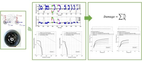
:The paper is devoted to the measurement and to the processing of load spectra of forces and moments acting at the wheel hub of a motorcycle. Smart wheels (SWs) have been specifically developed for the scope. Throughout the paper, the extreme case of a race motorcycle is considered. Accurate load spectra were measured in two race circuits. Standardized load spectra are derived by processing measured data. A way to easily generalize the measured load spectra is proposed for the first time for motorcycles. Several loading conditions, related to the motorcycle straight line motion, cornering, curb hit and gear shift, are identified and extracted from the experimental measures. For each loading condition, by means of simple semi-analytical models (SAMs), a relationship is found between the vertical force on the wheel, the tilt angle of the motorcycle and the remaining forces and moments acting at the wheel hub. Such relationships are nothing else than the standardized load spectra. Additionally, a simple and efficient method based on smart wheels for real-time structural monitoring is proposed. Standardized load spectra prove to provide consistent results even when compared to real-time structural monitoring data. By means of the presented smart wheels, advanced lightweight motorcycle construction is enabled by derivation of standardized load spectra or real time estimation of the damage of structural components.
1. Introduction
In this paper, we propose to use smart wheels (SWs) to derive load spectra for the design or for the structural monitoring of motorcycles. Using SWs for detecting external forces acting on a motorcycle enables in a straightforward way
- the derivation of load spectra,
- the derivation of standardized load spectra,
- the real time estimation of the damage of structural components.
1.1. Smart Wheels (SWs)
Referring to SWs, in previous papers, the authors have presented their activity in the field. SWs have been conceived, manufactured and employed extensively [1,2]. At the moment, the developed SWs are used for research or testing purposes. In the future, they could be industrialized to equip consumer motorcycles. A complete overview on smart wheels for motorcycle applications can be found in [3].
The special and unique characteristic of the SWs that have been used in this paper is their lightness. Contrary to other too heavy applications [2,3], the SWs that have been used in this paper provide practically the same forces at the hubs as normal wheels. This makes possible the derivation of reliable load spectra.
1.2. Durability and Derivation of Load Spectra of Motorcycles
Structural safety and durability are among the most important concerns of vehicle designers. Each vehicle component that is relevant for safety has to pass many tests before obtaining production approval [4,5,6,7,8,9,10]. Lightweight design has increased its importance in the last decades and nowadays is one of the main drivers in the design of new vehicles [11]. Obviously, mass reduction requires both special construction skills [12] and a deep knowledge and awareness of in-service loads.
The proper definition of test load spectra is the key point for designing safe lightweight automotive structures. Load spectra for trucks and passenger cars have been collected during the last 20 years [6,13,14,15]. In particular, Grubisic et al. ([16,17,18]) developed “Eurocycle”, a representative load spectrum of vertical and lateral wheel loads of European cars and commercial trucks.
A scarce literature is found on motorcycle durability [19,20,21,22,23]. In [19], a method for the fatigue life prediction of the frames of lightweight electric mopeds was developed. An experimental campaign was implemented to collect data from strain gauges installed at critical locations on the frame. Field tests on a total mileage of 300 km under various driving conditions (namely urban, extra urban, pavé, offroad and mountain) were conducted to extract a fatigue load spectrum of the frame. A fatigue life prediction based on the Miner linear damage summation rule was developed leveraging on additional indoor testing on a dedicated test bench.
Experimental acquisitions on a motorcycle frame were also used in [21] as reference input to reconstruct a fatigue load spectrum to be used for indoor testing.
In [23] the authors developed and validated a multi-body model of a moped. The model allows to predict the input loads acting on the main structural members of the moped during the roller-bench endurance test, one of the most widespread indoor tests among motorcycles manufacturers. In the paper, the authors provide load spectra of the vertical and longitudinal force acting on the moped.
1.3. Derivation of Standardized Load Spectra
The advantage in using standardized load spectra for designing vehicle components is acknowledged by Heuler et al. in two papers [24,25], where a comprehensive overview of existing standardized load spectra is provided and the principles applied for collection and analysis of appropriate load data, assessment of operating profiles and generation of the respective load spectra and sequences are discussed.
In the literature, there are many methods to obtain a standardized load-time history for four-wheel-vehicles, reference [26] refers to the CAr LOading Standard (CARLOS) sequence, maybe the most widely used load spectrum generator. In CARLOS, three uniaxial sequences of the vertical, lateral and longitudinal forces are to be applied on the front car suspension. According to this method, the three directional loads are independent, each one gives a different contribution to the suspension damage. In reference [27], the CARLOS sequence was improved by considering four load channels to solve the correlation problem.
In order to allow the experimental safety assessment of car wheels, Nurkala and Wallace [6] developed the standardized test spectrum for the well-known Biaxial Test rig, a standard repetition of 32 constant-amplitude blocks of vertical and lateral loads. The standard spectrum is adapted to the particular wheel to be tested by means of a scaling on the vehicle static load.
According to the known literature addressed above, to date, a well-established standardized procedure to derive load spectra for road vehicles is available only for cars.
Unfortunately, the known standardized procedures ([6,26]) require some adaptation that is not always complying with the physical dynamic behavior of the vehicle under consideration. Actually, the effect of the vibrations of the un-sprung masses [28] is generally neglected. In other words, the known standardized load spectra for cars and trucks do not consider accurately the influence of the suspension parameters (stiffness, damping). This is a shortcoming that is generally accepted to preserve the simplicity of the generation of standardized load spectra, letting them depend just on the static vertical force.
In the paper, we will propose standardized load spectra for motorcycles. The approach followed in the literature is followed, i.e., we will not consider the effect of vibration of un-sprung masses. Therefore, the standardized load spectra will depend on a limited number of parameters, namely the vertical load and roll angle of the motorcycle. We will discuss the simplifying approach and its pros and cons.
A method for combining forces and moments will be given. The method we propose overcomes the shortcomings common to some papers in the literature [6,26,27] which adopt scaling factors to consider different vehicles.
We review below a number of papers that deal with load spectra derived for motorcycles, all of them do not focus on standardized load spectra.
In reference [29], experimental tests on a maxi scooter have been conducted to collect data related to the in-service loads acting on the scooter subsystems. The acquired data have been employed to setup accelerated fatigue testing on a full-scale test bench. In reference [30], the authors instrumented several motorcycles with accelerometers to acquire data to be used to simulate real road inputs on an electro-hydraulic servo system test rig, aimed at studying the durability of a motorcycle frame. In [31], a methodology for estimating input loads on road motorcycles is presented and discussed. Input loads are estimated by exploiting a network of on-board sensors and a model-based approach. Estimated forces were validated through experimental data acquisitions. In [32,33], the authors instrumented the handlebar of a motorcycle with three-axis rosette strain gauges in order to obtain strain histories on several roads. The strain histories were then used as input for a servo-hydraulic actuator to obtain accelerated durability tests. The displacement histories applied by the test rig were obtained by reproducing the strain histories acquired on the motorcycle handlebar. Similarly, in [34], the authors instrumented a motorcycle with six strain gauges and two accelerometers to obtain load histories in order to develop an accelerated fatigue test. A motorcycle has been instrumented in [35] and [36] with strain gauges and accelerometers to evaluate the motorcycle fatigue strength by using a simulator. A study on the fatigue induced by structural resonance on motorcycle is presented in [37], the study takes advantage of data acquired from strain gauges on the frame. A motorcycle center stand has been instrumented in [38] to predict its fatigue life and optimize its design. In [39], a sport motorcycle was instrumented with strain gauges to measure the dynamic loads during the riding.
In all of the above papers referring to motorcycles, the load spectra have been estimated without resorting to a force sensor like a SW. In this paper, smart wheels (SWs) will be used to derive very accurately the load spectra.
The research activity presented in this paper is based on experimental measurements performed with a race motorcycle. The example of the race motorcycle has been chosen because the dynamical forces are extremely high. Forces at un-sprung masses are high during running on curbs. At the rear suspension, the forces are high due to driving torque.
The application of the method developed in this paper for consumer motorcycles should be relatively easy.
The motorcycle has been equipped with a set of SWs [1] to measure the tire/road contact forces. The acquired data have been processed to provide the fatigue load spectra of the forces and moments applied to the motorcycle as function of two standardized parameters only: the vertical force and the tilt angle.
1.4. Real Time Estimation of the Damage of Structural Components
Prognostic health monitoring (PHM) [40] may represent an attractive perspective in lightweight design. Considering the constantly increasing advance and complexity of automotive systems, sensors and components, a tool able to promptly detect faults, or provide a reasonable approximation of the remaining useful life of automotive parts, is fundamental for maximizing vehicle performances while maintaining an acceptable level of safety [41,42,43,44].
PHM aims to provide a real-time estimation of the Residual Useful Life (RUL) of a system, subsystem or component. In the framework of RUL predictions, two main different approaches can be distinguished in the literature, namely model-based approaches and data-driven approaches [45]. Model-based approaches rely on the availability of a validated physical model of the system under investigation, which is able to describe the damage process the system undergoes during its in-service life. Examples of analytical models of the fatigue damage of vehicle systems caused by road excitations can be found in the works of Gobbi and Mastinu [46] and more recently Jaoude [47]—in both of the works, the Palmgren–Miner linear damage accumulation rule was adopted.
Data-driven approaches, on the other hand, make use of monitoring data acquired during the whole life of the system (and with different levels of damage) and are preferred when a physical model of the damage process is unavailable, due for instance to the complexity of the process itself or the variability of operational conditions. Data-driven approaches require a large set of monitoring data and are generally based on probabilistic models that aim to identify trends by learning from the available data [48].
In the framework of data-driven approaches, extensive use of machine learning techniques is made, such as Neural Networks (NNs) or Radial Basis Function Networks (RBFNs). In a typical application, NNs are trained off-line on a “baseline” condition involving acquisitions during the early (and “healthy”) condition of the system [49]. However, differences that could occur between training conditions and real in-service life could significantly affect the accuracy of the method. Recently, adaptive prognostic approaches that combine Particle Filtering (PF) techniques and machine learning were proposed; the network parameters are identified online as soon as new observations are available, thus realizing an adaptive online training [49,50].
Data-driven approaches were extensively employed for the RUL estimation of composite structures [51,52,53]. In [51], the authors propose a probabilistic data-driven method for the RUL estimation of carbon/epoxy specimens subjected to a constant amplitude fatigue loading. The RUL model is based on Non-Homogeneous Hidden Semi Markov model (NHHSMM), which was improved in [48] by including adaptive features based on monitored data. In [52], a statistical life prediction method of composite structures is presented. The method takes advantage of Bayesian statistical theory to combine laboratory data with stiffness data measured on the in-service structure. The method was validated on both Glass Fiber Reinforced Polymers (GFRP) and Carbon Fiber Reinforced Polymers (CFRP).
Applications of data driven approaches extend also beyond purely mechanical problems, as the studies of Sbarufatti [50] and Liu [53,54] on Lithium-ion batteries demonstrate.
As a matter of fact, it is widely acknowledged that the uncertainty associated to the variability of operational loads, is one of the most important issues related to the practical implementation of structural monitoring and prognostics [42,43].
In such a framework, the SWs can provide accurate information on the actual input loads that are stressing the structure in any driving scenario. Concerning for instance the application described in this paper, the SWs can be included in the network of sensors and used to measure the actual input loads acting on the motorcycle subsystems, e.g., suspensions or motorcycle frame.
Once the input loads are known, a model-based approach [41] can be adopted to estimate the fatigue damage and the residual useful life of the structural components. Obviously, such an approach has to rely on the use of validated numerical models (based for example on finite elements and multi-body dynamics) that allow to calculate the applied stress on the mechanical components. The Palmgren–Miner rule can be finally adopted to calculate the fatigue damage and estimate the residual useful life of the components [46,55].
Additionally, data coming from the smart wheels could support the development of data-driven prognostic models, making the SW actual monitoring sensors that could help the model in the detection of a failure of a vehicle component.
1.5. Paper Structure
- -
- In Section 2, the smart wheels are briefly introduced.
- -
- In Section 3, the experimental tests and the acquired data are described.
- -
- In Section 4, the identified maneuvers and the motorcycle models employed for the simulations are described.
- -
- In Section 5, the standardized load spectra are calculated with the proposed method and compared with the ones obtained from the measured loads.
- -
- In Section 6, a possible application of the SW as a sensor for prognostic health monitoring of motorcycle structural components is envisaged.
- -
- In Section 7, a discussion is made on pros and cons of the proposed method for standardized load spectra of motorcycles.
2. Smart Wheel
In [1], a smart wheel rim is presented, suitable to be used as an instrumented wheel to measure the three forces and three moments acting at the hub. The complete set of generalized forces acting at the tire-road contact patch can be measured and the data can be provided with a very low latency to the vehicle.
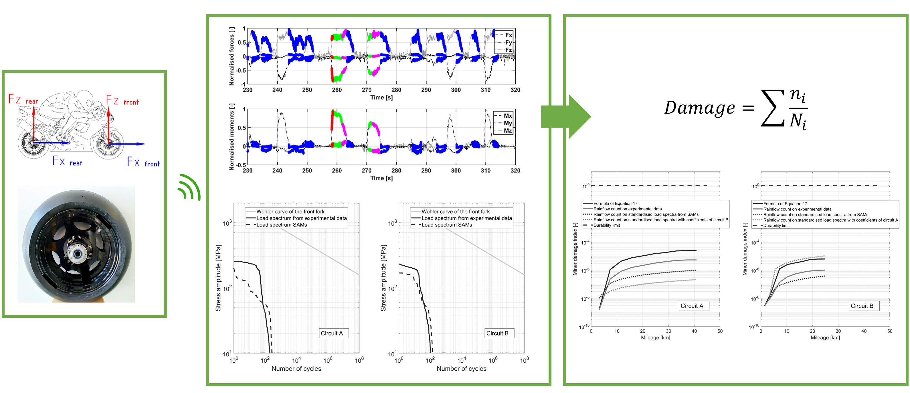
The smart wheel and its concept design are shown in Figure 1a,b, respectively. The three spoke structure that connects the central hub to the outer wheel rim in Figure 1a is the sensing structure. The sensing structure is constrained to the wheel rim by means of three joints positioned at the tip of each spoke. According to the scheme of Figure 1b, the sensing structure is statically determined in the space if and only if the joints at the three spoke tips are spherical joints able to translate in the direction of the respective spoke axes. This is the core of the invention [56,57,58]. Notice that the three spoke structure is ‘the’ optimal solution for making a rim a sensing structure. Actually, the three spoke structure is the only spatial structure to be statically determined and suitable for a wheel, two pre-requisites for obtaining the most accurate measuring performance.
In the actual embodiment (Figure 1a), the translating spherical joints that connect the sensing structure to the wheel rim are realized by means of thin laminae located between each spoke tip and the rim. Such kind of structures allow to obtain a low stiffness in the direction of the spoke axis with respect to the stiffness in the transversal direction, thus providing the sliding spherical joint constraint of Figure 1b. The shape of the laminae has been optimized in order to obtain translating spherical joints with some associated elastic stiffnesses. With this type of a structure, each spoke tip is subject only to the two forces T and N shown in Figure 2. A total of 6 forces are acting at the three spoke tips, the forces N1, N2 and N3 act along the y axis of Figure 2, while the forces T1, T2 and T3 act in the xz plane. Such forces can be measured by sensing the strain levels due to the bending moments at each spoke root, see Figure 2.
Given such six forces, the three forces and the three moments at the center of the wheel can be computed by solving simple equilibrium equations [58,59,60].
The three cantilever/spoke structure can be instrumented by means of 12 strain gauges at the basis of the spokes and connected in half-bridge configuration, as highlighted in Figure 2. Their positions have been defined in order to maximize the output (voltage) of the strain gauges for all combinations of loads applied at the wheel center. The strain gauges are intentionally located in the area where the bending moments acting at each cantilever/spoke produce high strains.
The SW has to be designed in order to have inertia properties (i.e., mass, moment of inertia) and stiffness similar to those of the standard wheels, provided that good sensitivity is provided.
As the measuring hub rotates, a telemetry system had to be designed and developed to transmit the six voltage signals from the strain gauges to a storage system on board of the vehicle.
Utilizing an encoder (angular resolution 0.05°), a simultaneous ADC sampling is performed on the six strain gauges bridges outputs while coupling the force/torque output with the absolute wheel angular position. The synchronous sampling allows seamless real-time measurements at vehicle speed up to 400 km/h.
The real-time calculation of the forces/torques components is performed by a DSP (Digital Signal Processor) programmed to apply the calibration matrix and the rotation matrix, as shown in the functional block diagram of Figure 3.
Referring to Figure 3, the voltage signals coming from the six Wheatsone bridges are amplified (gain G in Figure 3) and digitally converted (Analog to Digital converter in Figure 3). The digital signals are then fed to the DSP unit where they are multiplied by the sensor calibration matrix to calculate the output forces and moments in the wheel (rotating) reference system. To express the forces in the motorcycle reference system, a rotation matrix function of the wheel angular position is applied.
The signals are sent via Bluetooth to an on-board receiver connected to the vehicle CAN bus. Each signal can be sampled at 1600 Hz and more. Oversampling rate (1.6 kHz) has been selected such that anti aliased frequencies are below the noise floor allowing to eliminate the need of analog filters with the advantage of reducing the time delay associate with analog PB filtering. The acquired signals are then digitally low pass filtered at 90 Hz and broadcasted via the CAN network at 200 Hz per channel.
The accuracy of the smart wheel is very high, the resolution is 1 N and 0.1 Nm for force and moment, respectively. The linearity full up to the hysteresis is extremely reduced, the full-scale error is 1%, the uncertainty is 1.5% in every condition.
3. Experimental Tests
A race motorcycle has been equipped with two smart wheels, presented in [1]. These wheels are instrumented with a set of strain gauges and allow to measure the three force components and the three moment components applied at the wheel center (Figure 4). In addition, the tilt angle and the motorcycle speed are acquired. All the data are collected by an on-board data logger via CAN-BUS.
A professional rider drove the motorcycle, in a race-setup configuration, on a race circuit (referred to as circuit A hereafter). Data related to ten consecutive laps were acquired, for an overall mileage of about 40 km.
From the analysis of the acquired data, five different typical running conditions have been identified, which represent relevant loading conditions of the motorcycle. They are
- #1.
- pure longitudinal motion
- #2.
- steady turning
- #3.
- combined longitudinal and cornering
- #4.
- curb hit
- #5.
- gear shift
In the pure longitudinal motion, the motorcycle is either accelerating or braking on a straight path. The longitudinal force will be either a traction or a braking force.
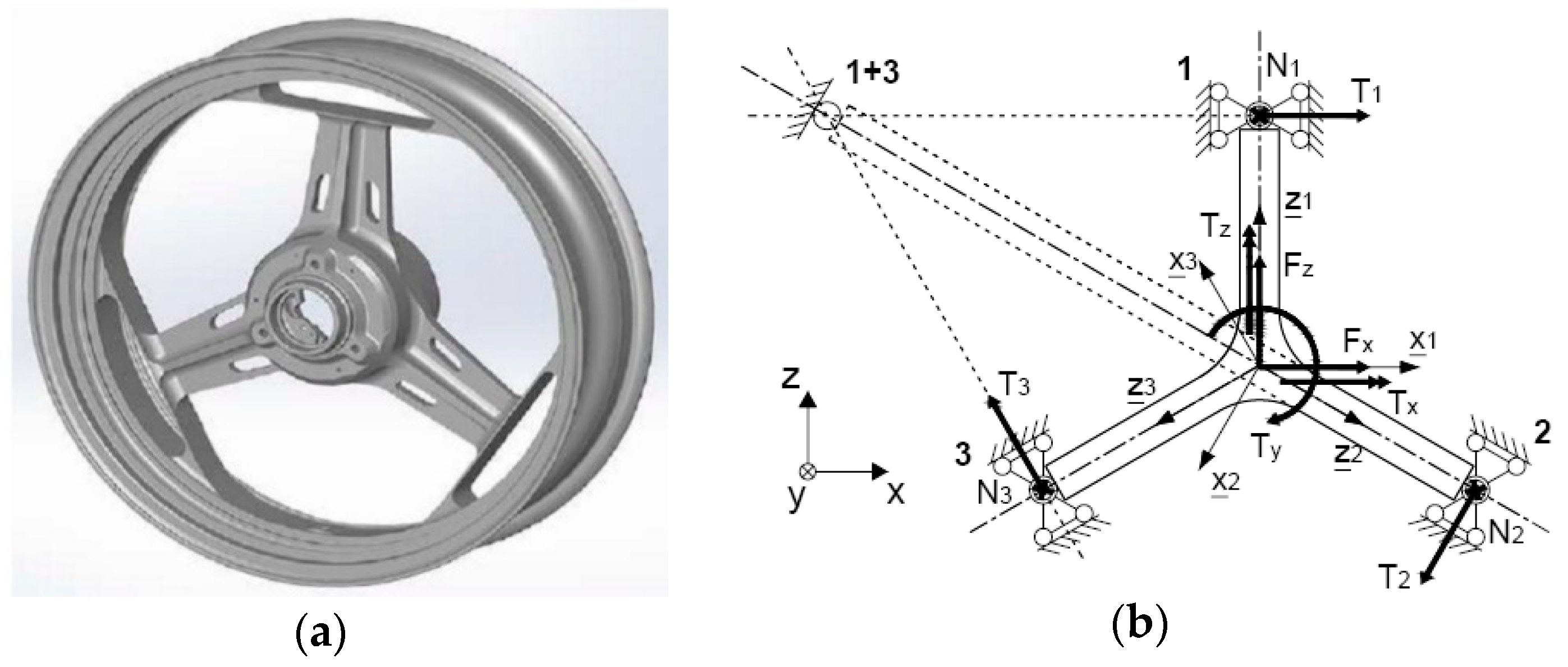
In the steady turning, the motorcycle is in a pure cornering situation, with no tractive or braking force. The tilt angle ( in Figure 4) is high and the speed is assumed to be almost constant in this phase.
The combined longitudinal and cornering condition refers to a case in which both longitudinal and lateral forces are applied at the ground. This condition is reached either at the beginning or at the end of a corner, where, respectively, the driver is still braking while approaching the turn, or is accelerating at its exit.
In the curb hitting, the motorcycle is passing over a curb, this generally happens during a corner, where the driver passes firstly over the inner curb and then on the outer curb at the corner exit.
In the gear shift, an instantaneous peak of the longitudinal force is measured on the rear wheel. This force is caused by an overshoot of the engine torque transferred to the wheel through the driveline, which occurs every time the driver acts on the gearbox lever to shift the gear.
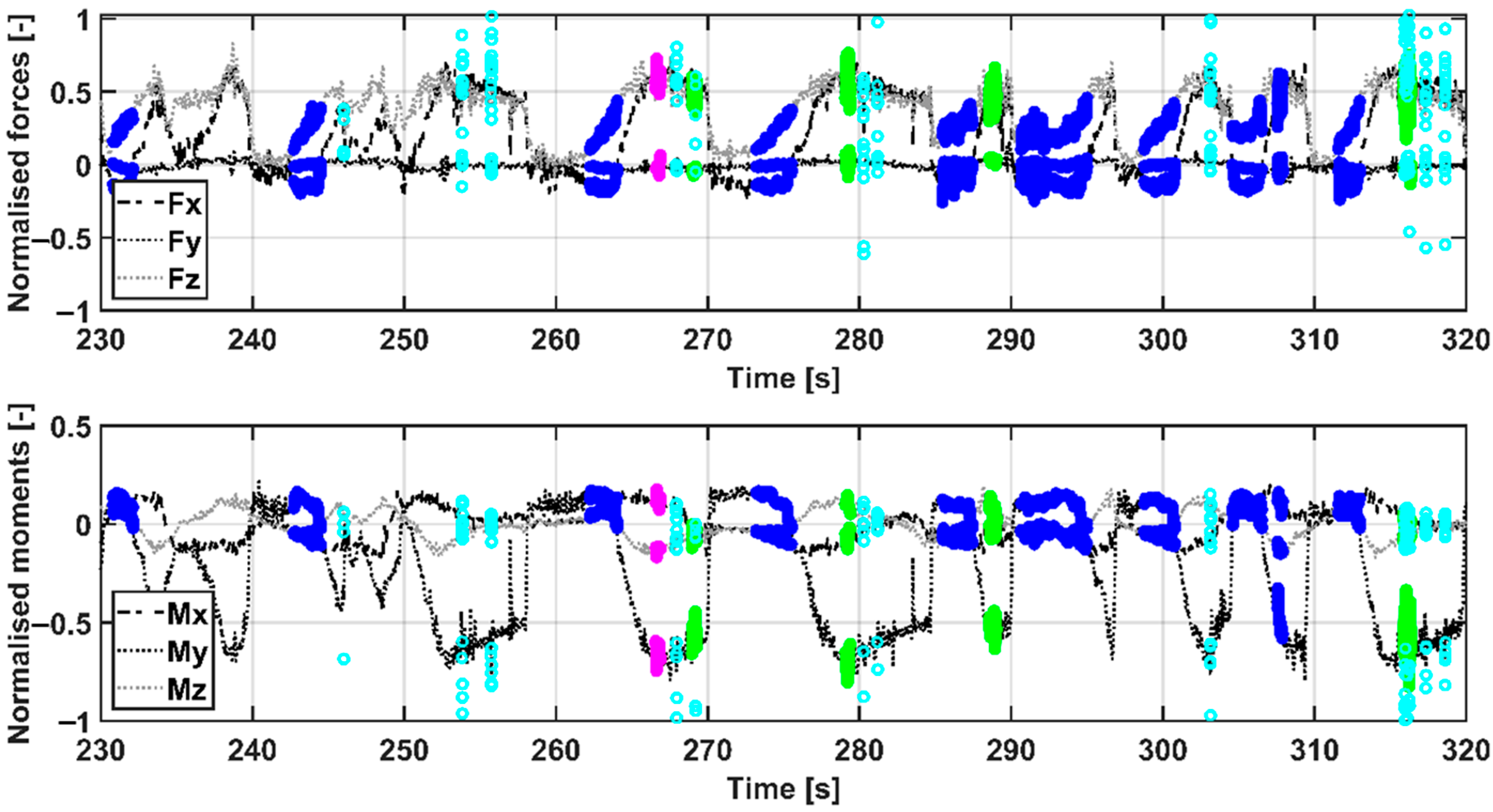
Figure 5 and Figure 6 depict the signals of the forces and moments measured by the rear and the front SWs respectively; the data refer to a single lap of circuit A. In the graphs, the five running conditions are highlighted. The identified running conditions cover almost the entire portion of the lap acquisition, meaning that they are representative of actual in-service loading conditions of the motorcycle.
4. Motorcycle Semi Analytical Models
In this section, simple semi-analytical models (SAMs) able to describe the motorcycle dynamic behavior in the defined running/loading conditions are developed. The developed models are either based on simple equilibrium equations of the motorcycle, or on linear regression models applied to the acquired experimental data. The inputs of the models are the vertical loads acting at the front and rear wheel and, where required, the motorcycle tilt angle. The models are quasi-static, no effect of the vibrations of the un-sprung masses is introduced to keep the derivation of load spectra as simple as possible.
The models give as output all the remaining relevant forces and moments acting at the wheel center for each running/loading condition. The models consider the motorcycle as a single, rigid body, i.e., the dynamics of other motorcycle subsystems, like suspensions and engine vibrations, are neglected. This limitation of the models allows to avoid to introduce many parameters (e.g., suspension stiffnesses and damping, tires, etc.) and have somehow general and robust estimates of the load spectra. However, we have a good estimation of the motorcycle loads only in the low frequency range (up to few Hertz), which is the most relevant for fatigue.
In this paper, the experimental data acquired by the SWs are filtered down to 1 Hz and used to calibrate the SAMs. Experimental data could be easily processed at higher cut-off frequency to explore the effect of high frequency loads on the fatigue damage, but this would imply a more complex modeling with errors eventually introduced by the uncertain parameters.
The final aim of these models is that of reconstructing suitable load spectra starting from simple data of the vertical load and the tilt angle, which can be obtained by simple and cheap sensors mounted on the motorcycle.
This is a way to standardize loading conditions and related load spectra. Actually, given the vertical force on the wheel (and the tilt angle), the other remaining forces and moments can be easily derived.
In the following, all of the SAMs and their tuning on experimental data acquired by SWs are described and analyzed.
4.1. Pure Longitudinal Motion (Running Condition #1)
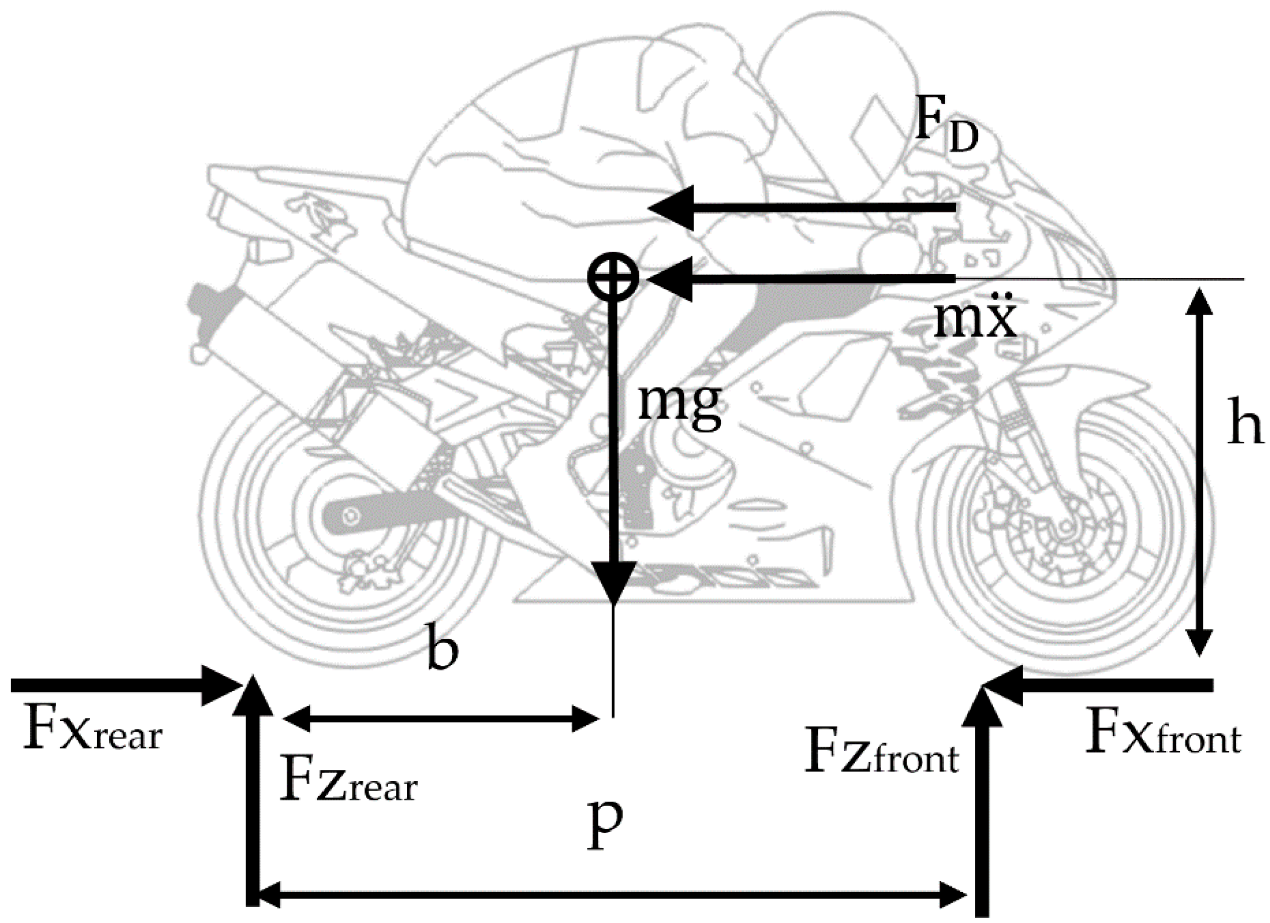
The load transfer motorcycle model described in [61] and shown in Figure 7, is adopted. In this model, the following hypotheses are assumed:
- -
- the rolling resistance force is neglected,
- -
- the aerodynamic lift force is neglected,
- -
- the aerodynamic force FD is the only resistance to the forward motion of the motorcycle,
- -
- the rotational inertial effects are neglected,
- -
- the longitudinal and vertical forces act at the tire/road contact points.
The geometrical and mass properties of the motorcycle are reported in Table 1.
From the model of Figure 7, the following three equilibrium equations can be written
In case of straight path acceleration, is neglected, while for braking, is vanishing. In both cases, the aerodynamic resistance is neglected.
Therefore, for straight path acceleration, the longitudinal force Fx and the moment My can be expressed as a function of the only vertical load Fz through the linear relations of Equation (2)
For rectilinear brake, Equation (3) holds
The coefficients α1, α2, α3 and α4 are correction factors that are to be identified from the forces measured by the SWs during this particular loading/running condition.
For the identification of α1, α2, α3 and α4, the measured signals acquired by the SWs are used. To extract the signals of running condition #1 from full time histories, thresholds for the tilt angle, the vertical force Fz and the moment My, have been defined and reported in Table 2 and Table 3, respectively for the rear and front wheel.
The coefficients α1, α2, α3 and α4 are identified by means of a least square fitting on the measured quantities. The identified values are reported in Table A1 in Appendix A.
4.2. Steady Turning (Running Condition #2)
To describe this maneuver, the motorcycle model of Figure 8 is adopted [61]. In the model, the following hypotheses are assumed
- -
- the tire geometry is neglected, i.e., the tires are assumed as rigid planes,
- -
- the motorcycle speed and lateral acceleration are constant,
- -
- the gyroscopic effects are neglected,
- -
- the lateral load Fy is equally distributed on the front and rear wheel.
The following equilibrium equations can be written
where , and are identified from the acquired experimental data. In this case, to extract the time histories for the identification, the thresholds on the tilt angle, on the vertical force Fz and on the moment My that are reported in Table 2 and Table 3 are considered. The correction coefficients are then identified as described above. The identified coefficients are reported in Table A1 in Appendix A.
4.3. Combined Longitudinal and Cornering (Running Condition #3)
In this running/loading condition, a combination of traction or braking force and cornering is experienced. The model employed for describing such a condition is a simple superposition of the two models described above (Figure 7 and Figure 8).
Equations (5) and (6) define the forces acting at the wheel center, respectively, for an acceleration at the turn exit and a brake while entering the turn.
The coefficients (i= 9,…,16) in Equations (5) and (6) are correction factors that are identified by a least square fitting on experimental data. The motorcycle geometrical and inertial properties are summarized in Table 1.
4.4. Curb Hit (Running Condition #4)
During the lap, the rider often passes over the curbs located at the sides of the track. In this phase, a rapid increase of the vertical and longitudinal force is highlighted by the experimental acquisitions. In order to detect the curb hitting, a moving average filtering approach is employed. A sliding time window of 0.2 s is defined and the root mean square of the combination of vertical and longitudinal load defined by Equation (7) is computed.
The selection of the sliding time window depends on many factors, such as motorcycle velocity and curbs profile, that are related to the particular track on which the motorcycle is running. The selection process of the sliding time window starts by considering a reference value of about 0.1 s, which is then iteratively tuned by analyzing the acquired experimental data.
The computed value of the RMS of Equation (7) is then compared with the mean value of the RMS of all the sliding intervals considered in the time history. If the computed RMS is greater than 3 times the mean RMS (Equation (8)), that interval is considered as a curb hit.
Since the curb hitting occurs either during a straight line driving or during a turn, each one of the three models described above (i.e., pure longitudinal motion, steady turning and combined longitudinal and cornering) can be employed to compute the wheel forces.
4.5. Gear Shift (Running Condition #5)
In the acceleration phases, to minimize the gear shift time, the rider does not disengage the engine from the driveline. This use of the gearbox provides a high peak of the torque transmitted along the driveline, which is felt as an instantaneous peak on the moment My measured by the rear wheel. The identification of this loading condition happens in a similar way as for the curb hitting, but, due to the fast dynamics of the maneuver, the sliding interval for the RMS calculation has been reduced to 0.05 s, and the threshold value for the RMS comparison has been increased to 7. As for the case of curb hit (running condition #4) the selection of the time window is done iteratively by analyzing the acquired time histories. The RMS is now calculated on the torque My measured by the rear wheel as shown in Equation (9).
The torque My must be higher than 800 Nm and the minimum duration time is set to be greater than 0.005 s.
For this load case, a simplified relation has been adopted to correlate the longitudinal force Fx and the moment My on the rear wheel with the vertical force Fz. The other loads (i.e., Fy and Mx), being significantly lower, are neglected for this loading condition. Two correlation coefficients have been introduced as shown in the expressions of Equation (10).
Equation (10) provides a relation between the traction torque Myrear (and therefore the longitudinal force Fxrear) and the vertical force Fzrear applied to the rear wheel. From the physical point of view, such a relation is explained by the peak of the driving torque My and longitudinal force Fx during the gear shift, which effect the motorcycle longitudinal and vertical motion.
The correlation coefficients are calculated by means of a least square fitting on the acquired experimental data. The identification thresholds are summarized in Table 2, while the values of the coefficients are reported in Table A1 in Appendix A.
5. Results and Comparison
In the previous section, numerical coefficients (i = 1,…,34) are introduced to minimize the least square errors between the experimental loads and the forces computed by SAMs. Such numerical coefficients are used to recover the simplifying hypotheses that were introduced for SAMs.
All the identified coefficients are reported in Table A1 in Appendix A. Tests have been performed in the race circuit A.
From the acquired experimental data, the load spectra of the forces and moments acting at the front and rear wheel of the motorcycle are calculated. The Rainflow cycle-counting method [62] has been adopted to extract the mean and alternate components of the loads and the respective number of cycles. The load spectra have been computed over 10 laps on circuit A, for an overall mileage of about 40 km in real race conditions.
Figure 9 shows the load spectra related to the vertical force acting at the front and rear wheel for the 10 considered laps. The histograms are computed by dividing the alternate and mean components of the vertical force into classes of amplitude of 200 (N) or 200 (Nm). In the obtained graphs, all the contributions related to the loading conditions identified in Section 4 are included.
The experimental time histories of the vertical forces acting at the front and rear wheel and the signal related to the tilt angle, are fed to the motorcycle models described in Section 4, which provide the time histories related to the remaining force and moment components for each loading conditions. The Rainflow counting method is then applied to the obtained time histories to calculate the load spectra of the simulated forces and moments acting at the motorcycle wheels.
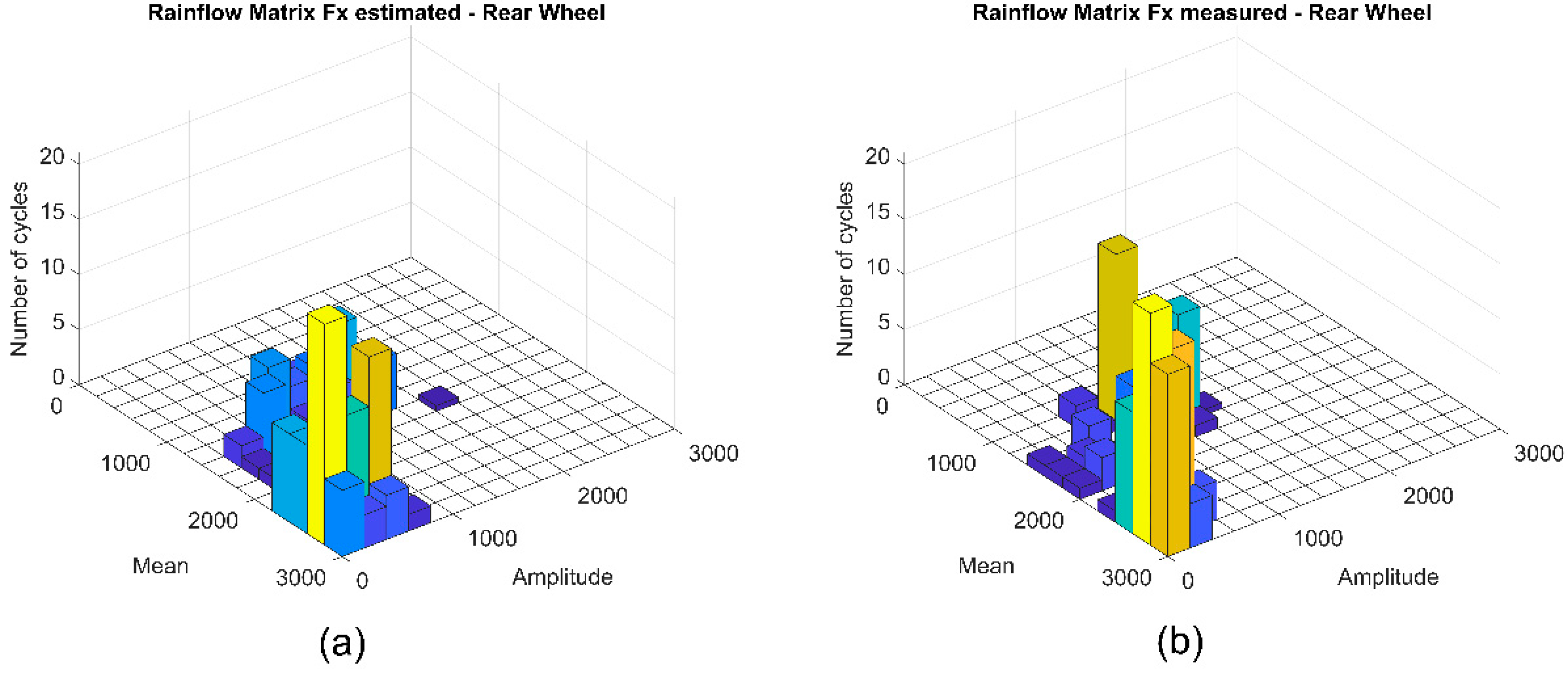
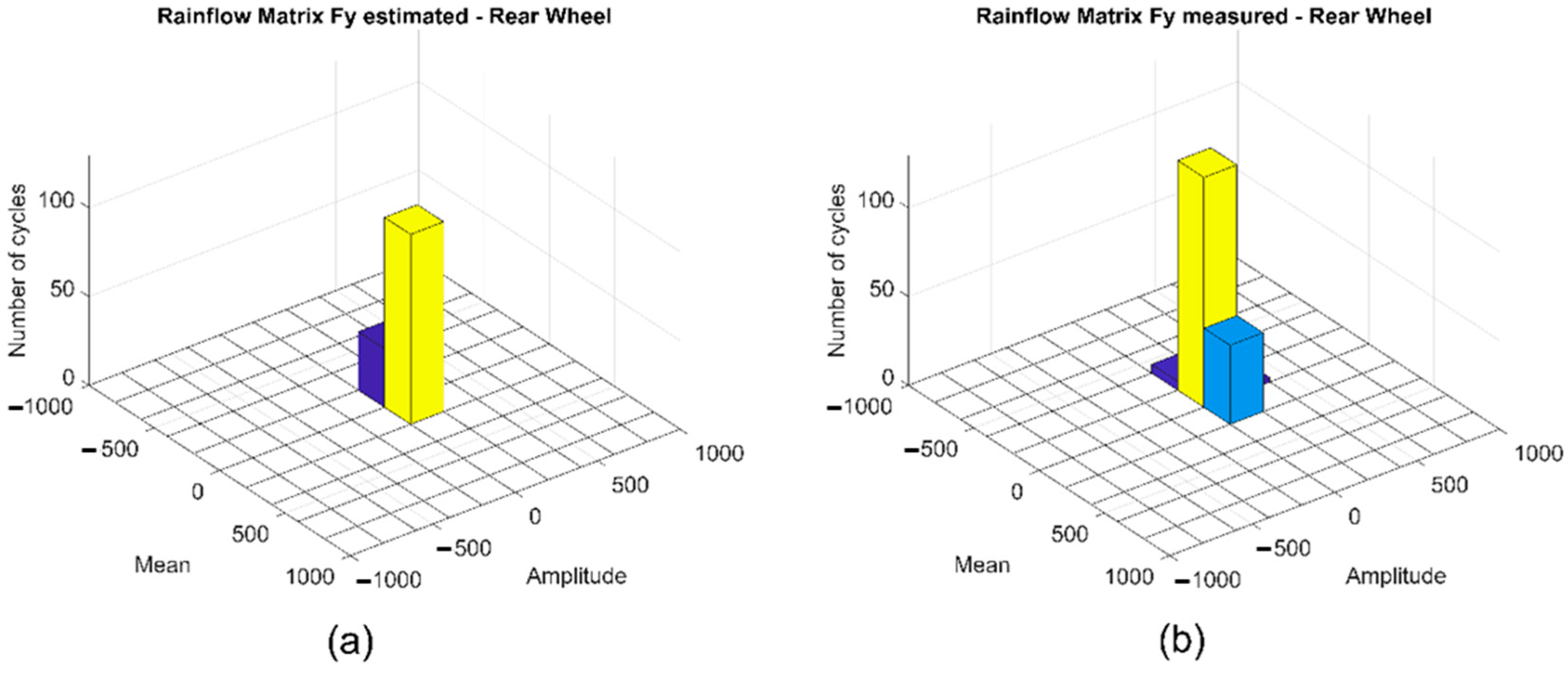
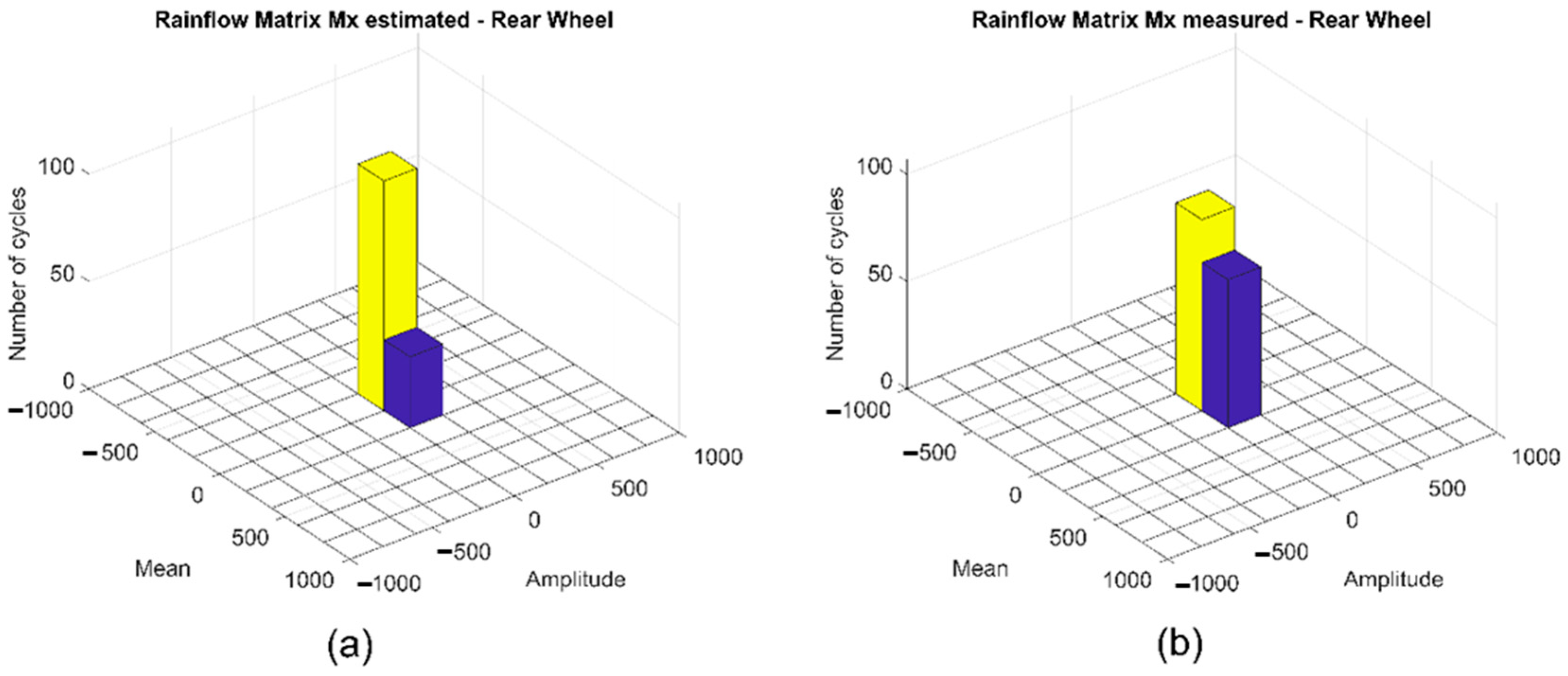
In Figure 10, Figure 11, Figure 12 and Figure 13, the comparison between the load spectra of the rear wheel obtained from experimental data and from the simulations by SAMs is reported for the longitudinal force Fx, the lateral force Fy, the tilting moment Mx and the torque My, respectively.
The comparison of the obtained load spectra shows a reasonable correlation between experimental data and analytical models, in terms of both mean and alternate components of the loads and in terms of related number of cycles.
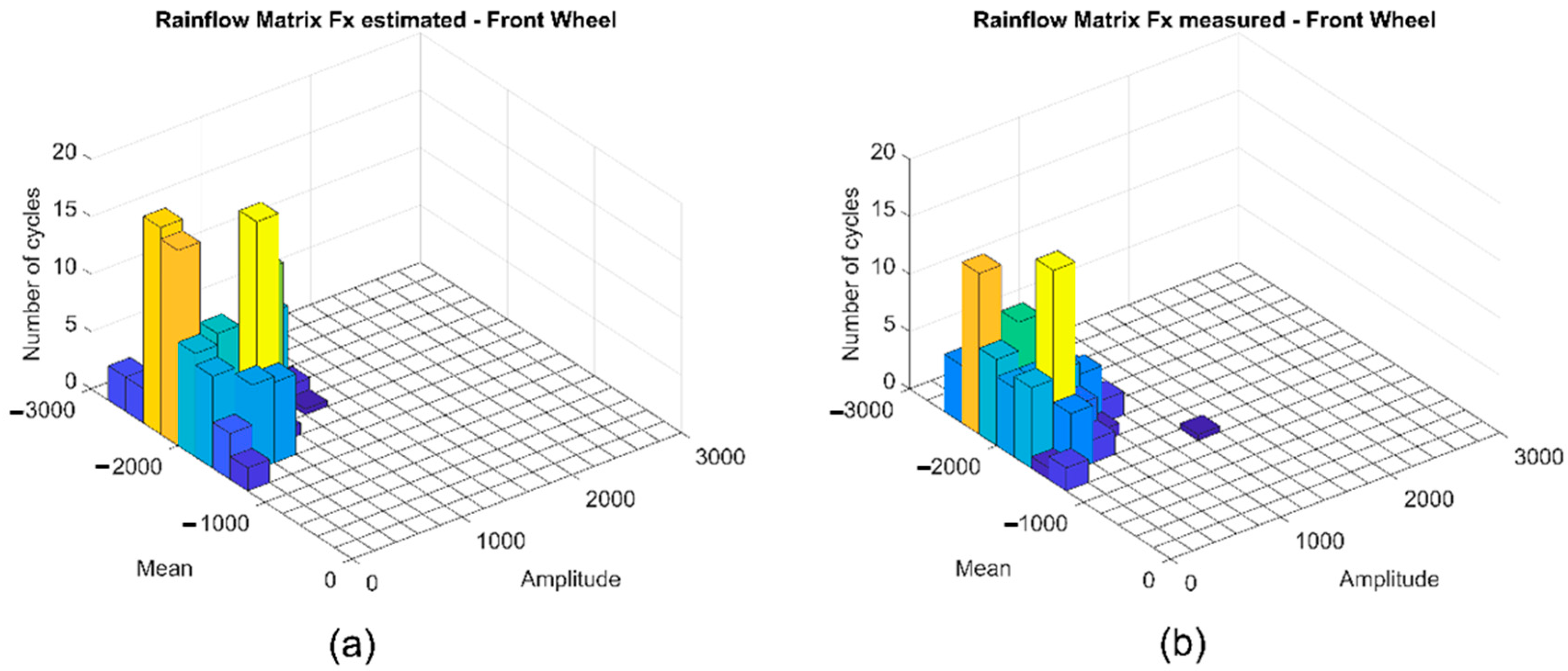
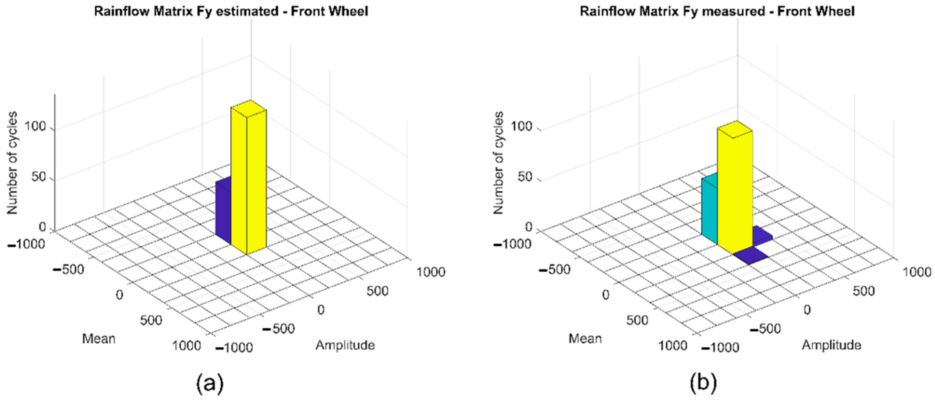
Figure 14, Figure 15, Figure 16 and Figure 17 show the comparison of the load spectra of the forces and moments acting at the front wheel. Even in this case, a reasonable correlation can be highlighted.
At a first inspection, the load spectra coming from the bare measurements and the standardized version given by SAMs are just approximately similar. This is due to the fact that, to keep the standardization as simple as possible, we used a quasi-static formulation for SAMs. We will see in Section 6 that the damage computed by the Miner’s rule is similar for measured load spectra and for SAMs load spectra.
To check the robustness of the information obtained by SAMs, data coming from a different circuit (named circuit B in the following of the paper) have been considered. These data refer to the same motorcycle, but with a slightly different setup, running for 10 consecutive minutes (5 laps) on a completely different race circuit.
Considering the new data acquisitions, different coefficients αi have been identified for the SAMs. Comparing the new identified αi with the ones of circuit A, a variation of less than 15% has been found for the standard running conditions (i.e., running conditions #1, #2 and #3). Regarding running conditions #4 and #5 (curb hitting and gear shift), the maximum difference on the identified coefficients rises up to 35%, probably due to the different profiles of the curbs of circuit B and the different strategy adopted for gear shifting.
The limited difference in the identified coefficients however demonstrates the effectiveness of the approach in deriving standardized load spectra of race motorcycles, provided that a sufficiently large set of data from different circuits is available.
6. Smart Wheel as a Sensor for Prognostic Health Monitoring
The stress level (s) in a generic motorbike component can be evaluated from the external forces and moments acting at the wheels: Fx,front Fy,front Fz,front, Fx,rear Fy,rear Fz,rear, Mx,front My,front Mz,front, Mx,rear My,rear Mz,rear. Let us consider the transfer functions H(s/Fik) and H(s/Mik) where I = front,rear and k =x,y,z and s is the stress at a certain location of a certain component. The transfer functions depend on the shape of the component
where A = F,M, I = front,rear and k = x,y,z. The combined effect of the loads Fx,y,z,front, Fx,y,z,rear, Mx,y,z,front and Mx,y,z,rear acting simultaneously can be computed by applying the superposition principle.
The power spectral density of the stress is
where is the power spectral density (PSD) of the applied loads as function of the angular frequency (ω).
The component suffers an amount of damage which can be expressed as
where n is the number of cycles at constant stress amplitude s, N(s) is the number of cycles to failure at stress amplitude s obtained from the Wöhler’s curve Nsk = C, and D is the damage function.
According to Miner’s rule if Di is the fraction of damage caused by ni cycles at stress level si given by
the total cumulative damage D is given by
and the failure should occur when D = 1.
The main criticism to this approach is that the loading sequence and stress interaction effects are disregarded, resulting in non-accurate estimates of fatigue life. Nevertheless, due to the simple formulation, it remains a useful approach for the real time estimation of the damage level of the component.
The total expected damage in the time interval T for a stationary Gaussian random process is upper-bounded by the following formula presented in [63] by Rychlik
where Γ () is the Gamma function, λ2 is the stress spectral moment of order two, λ0 the stress spectral moment of order zero and C and k the Wöhler’s curve parameters of the material (Nsk = C). However, it is widely acknowledged that the upper bound provided by Equation (16) may give over-conservative results for wide-band processes [64]. That is why in [64] a corrected version of Equation (16) was provided, which gives an improved estimation of the fatigue damage level under the assumption of a Rainflow count and linear damage accumulation
where the weight can be computed as
and depends only on the PSD bandwidth parameters and :
where and are the stress spectral moments of order one and four, respectively.
Example: Estimation of the Fatigue Damage on the Front Fork
In this section, an example of fatigue life estimation is discussed. The example refers to the structural health monitoring of the motorcycle front fork. The damage of the front fork has been calculated both for circuit A and circuit B.
The forces and moments signals acquired by the front SW during the on-track tests are filtered down to a frequency of 1 Hz with a 4th order Butterworth filter. The filtered signals are then combined to calculate the stress acting on the fork.
The total expected damage level is computed in two ways, by the formula of Equation (17) or by the Rainflow counting on the stress time history. Additionally, the same damage index is calculated considering the standardized load spectra derived from SAMs and presented in Section 5.
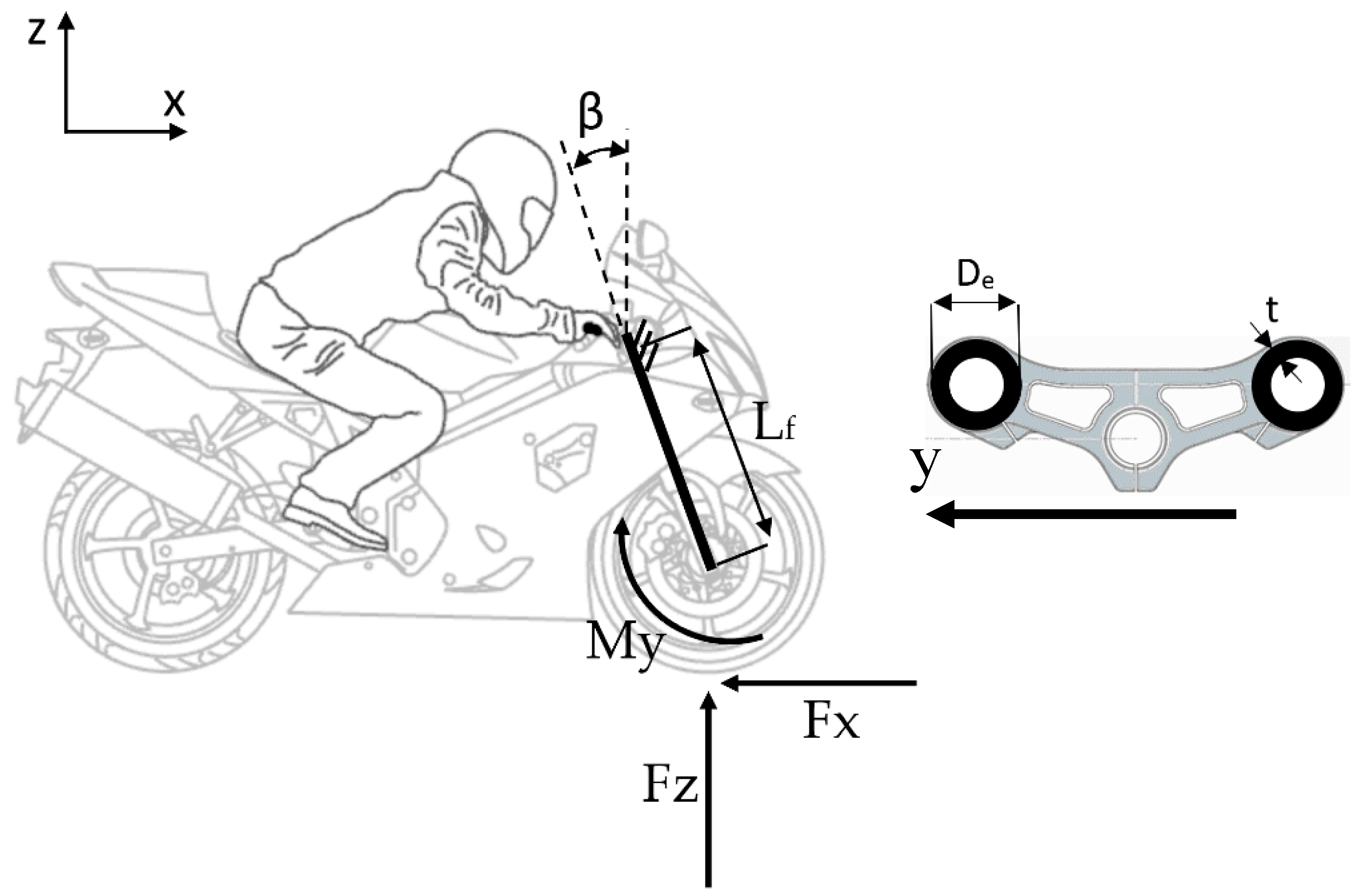
The front fork is made by two circular tubes made from 34Mn5 low alloy steel. The analyzed system is depicted in Figure 18 and can be schematized as a cantilever beam with a free loaded end. The geometrical parameters of the front fork are reported in Table 4.
Referring to Figure 18, the maximum bending stress acting on the fork stems in the x-z plane reads
where is given by the ratio of the moment of inertia of the cross section and the maximum distance from the neutral axis (the factor 2 accounts for the two stems). The bending stress acting on the x-y plane is more than 20 times lower than the one of Equation (20) and is therefore neglected in the computation.
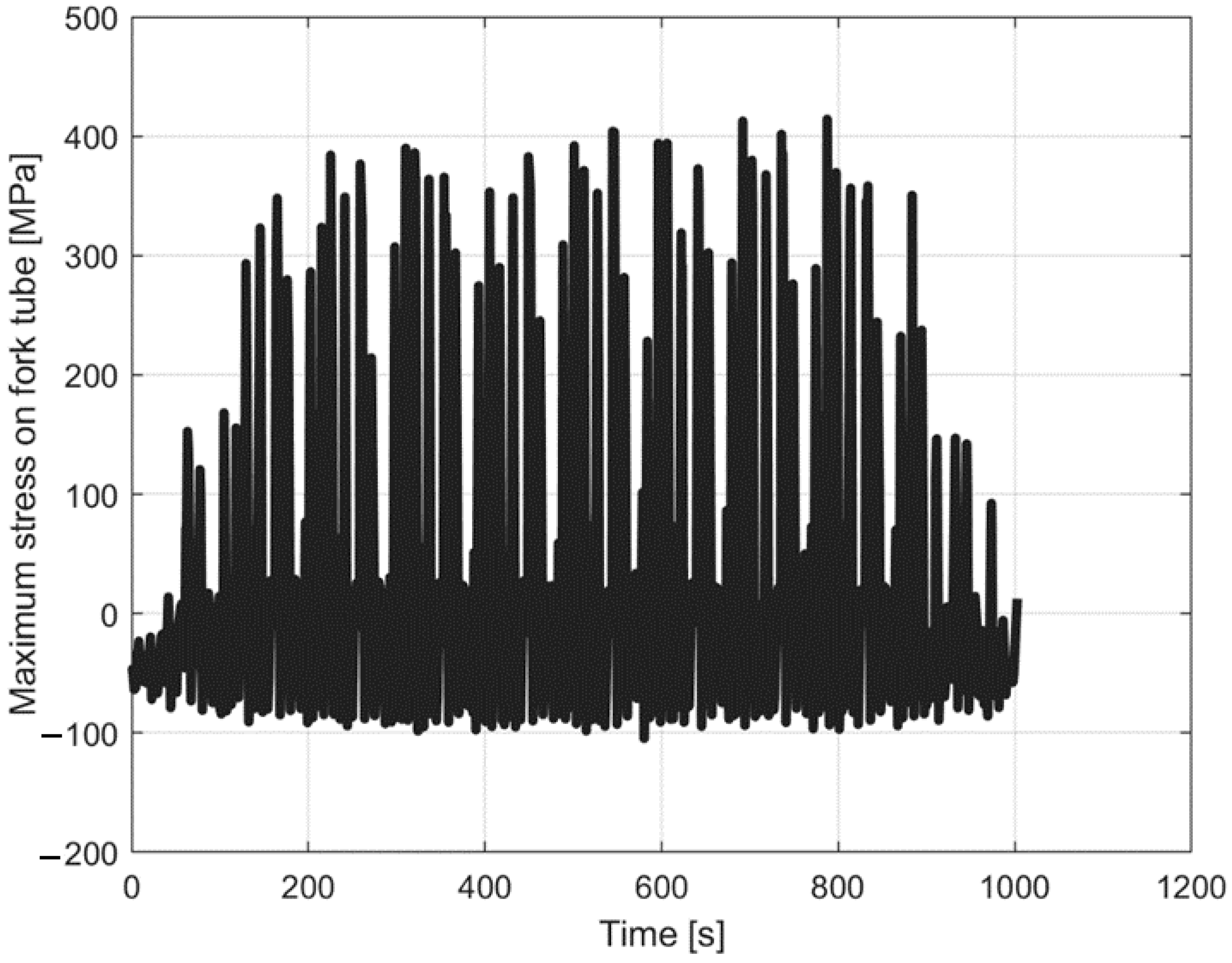
An example of time history of the maximum bending stress computed from the experimental data acquired by the front SW during the tests on circuit A is shown in Figure 19.
The maximum number of cycles to failure of the fork depends on the fatigue properties of the 34Mn5 low alloy steel and on other factors, such as: the local stress concentration factor (set to 1 for sake of simplicity here), the dimensions of the fork, the surface finishing. Dimension and finishing are taken into account by introducing two parameter coefficients, b2 and b3, respectively.
Assuming a typical endurance limit of approximately 400 MPa, a slope of the Wöhler’s curve k ≈ 7, b2 ≈ 0.9 and b3 ≈ 0.9, the numerical value of C equals 2.39 × 10²³ (C is the parameter of the Wöhler’s curve Nsk = C).
The fatigue stress amplitude acting on the stems can be calculated by simply deducting the average stress from the time history (Figure 19). The PSD of the obtained signal is then employed to compute the four spectral moments λ0, λ1, λ2 and λ4 that appear in Equation (19).
The described procedure has been applied to portions of the stress time history, with T ≈ 100 s. The damage index of each portion of the signal is calculated from Equation (17) and the total damage at the end of the test is given by the sum of each contribution.
The second approach that has been employed for the fatigue life estimation of the component is based on a Rainflow counting method. In this case, the stress cycles are directly extracted from the time history (Figure 19). The damage level is then evaluated by applying Equations (14) and (15). For this second approach, also the standardized load spectra derived from the SAMs and presented in Section 5 have been considered.
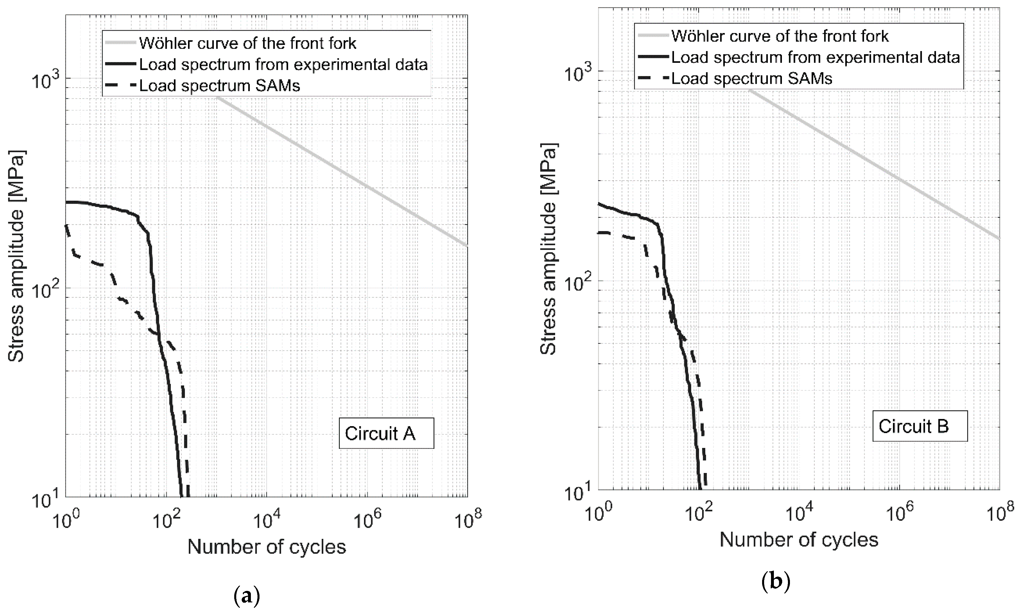
Figure 20 depicts the spectra of the stress amplitude acting on the fork stem, computed from both the experimental time histories and the standardized load spectra derived from the SAMs. The plots of Figure 20 refer either to circuit A (Figure 20a) or circuit B (Figure 20b). In the figure, the Wöhler’s curve of the fork stem is shown as well.
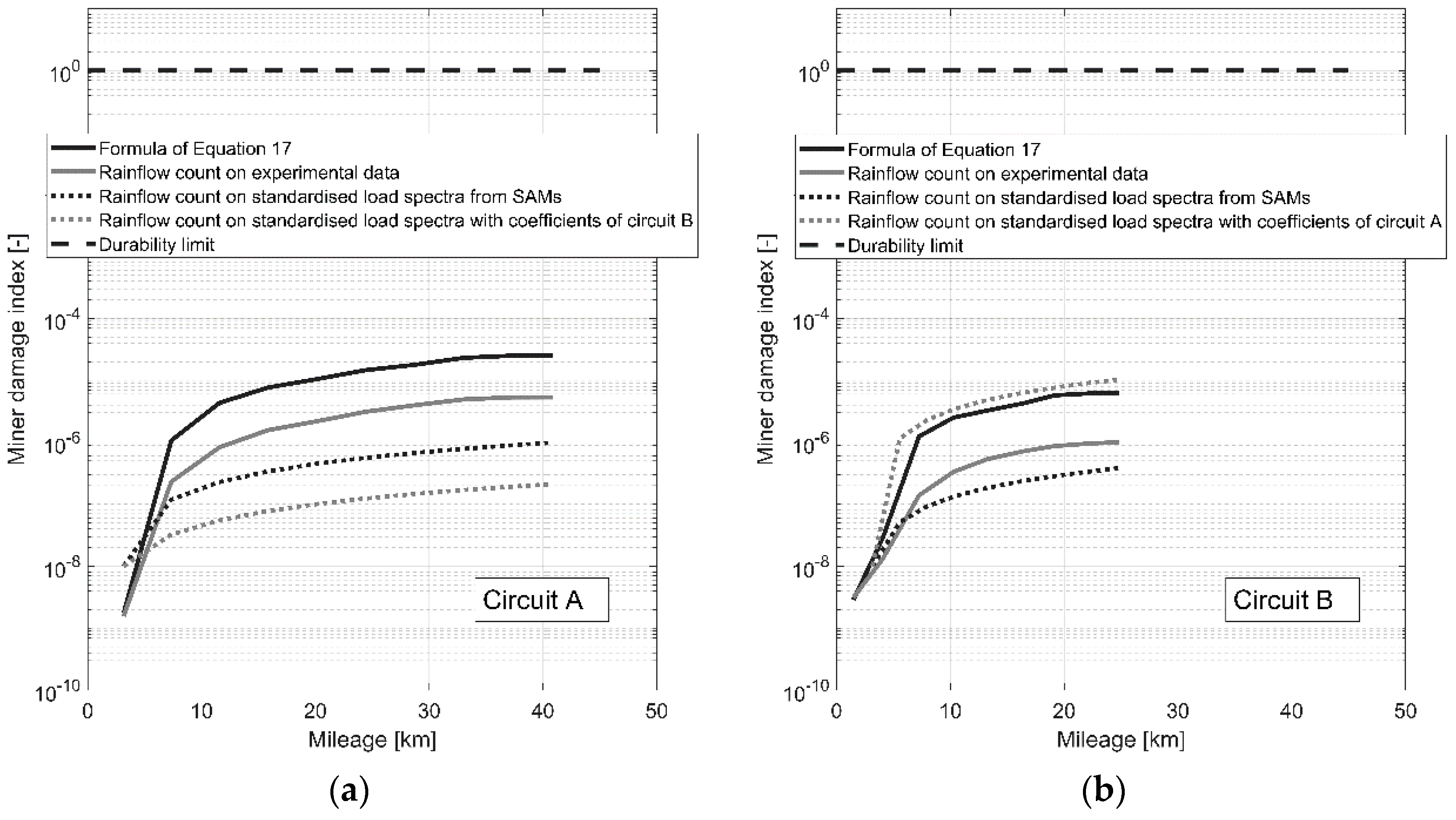
Figure 21 shows the evolution of the fatigue damage index of the front fork as function of the covered mileage, computed with the two described approaches on either circuit A (Figure 21a) or circuit B (Figure 21b). In Figure 21, the grey solid lines refer to the calculated Miner damage index after Rainflow counting from experimental data. The black solid lines refer to the Miner damage index computed with Equation (17). The black dashed lines show the Miner damage index computed from the standardized load spectra derived from SAMs and described in Section 5. The grey dashed lines show the Miner damage index computed from the standardized load spectra derived from SAMs with indices αi, which are derived from the data of another circuit. In other words, the grey dashed line pertaining to circuit A is derived with parameters αi identified on circuit B, and vice-versa.
By analyzing the plots of Figure 21, several comments can be made.
- -
- For all cases, the damage level is well far below the unit value, which means that the front fork is able to withstand the loads applied along the covered mileage without any durability issue.
- -
- Concerning the damage levels computed from experimental data, it turns out that Equation (17) provides a more conservative prediction than the Rainflow approach, with a damage level equal to 2.50 × 10⁻⁵ against 0.53 × 10⁻⁵ for circuit A and 6.19 × 10⁻⁶ against 1.00 × 10⁻⁶ for circuit B. This was however quite expected, since Equation (17) provides an upper bound of the fatigue damage level.
- -
- Concerning the damage level computed from the standardized load spectra, results show that the SAMs tend to provide a less conservative prediction than the experimental data. If for instance the rainflow count on the standardized load spectra of circuit A is considered (the black dashed line in Figure 21a), it can be seen that the computed damage index is about five times lower than the result obtained with Rainflow count on experimental acquisitions (the grey solid line in Figure 21a). For circuit B, the ratio between the two computed damage indices is around 2.6.
- -
- In case the parameters αi pertaining to a circuit are used to derive the damage on the other circuit, the damage may vary of more than an order of magnitude. It can be seen that, for circuit A, the two values are still comparable (the damage level goes from 9.88 × 10⁻⁷ to 2.11 × 10⁻⁷), while for circuit B a larger difference is experienced. These discrepancies could however be reduced by considering averaged values of the αi on a large set of data coming from different circuits.
From the practical point of view, both of the two described computational methods can be implemented into any Digital Signal Processing unit, enabling an almost real time computation of the damage level of the motorcycle components. Equation (17), although more conservative, has indeed important advantages in terms of computational effort, since it simply requires to update the values of the spectral moments as soon as new samples are available. The Rainflow Counting approach, on the other hand, requires the whole signal to be stored in memory to compute the stress load spectrum once the prescribed time period T is reached.
7. Discussion
One aim of the paper was to derive load spectra for motorcycles by measuring directly the loads at the wheels. The enabling technology was provided by proper smart wheels (SWs) able to produce reliable data. This seems an original contribution. Without light smart wheels the forces acting at the motorcycle are derived in a too approximated way, as the attempts made in the literature show.
Additionally, we did want to produce, for motorcycles, standardized load spectra, i.e., load spectra depending on few parameters (namely vertical load and tilt angle). This contribution seems quite original, and useful in the concept design phase. The designer can produce a preliminary structural arrangement without having tested the physical motorcycle. We did propose a method to derive such standardized load spectra by resorting to simple semi-analytical models (SAMs). The shortcoming here is that to keep the standardized load spectra as simple as possible, the forces related to the vibrations of the suspensions or driveline had to be neglected. This produces -as expected- slightly lower damage than the one computed by actual measured load spectra. Nonetheless, an engineering scaling factor of 5 (reasonable when we consider damaging effects [24]) could be used to exploit effectively the derived standardized load spectra for motorcycles. A broad test campaign could be organized to set the scaling factor, but this is out from the scope of this paper.
We have seen that changing the race circuit the damage can vary considerably. This has a direct effect on parameters αi. This means that parameters αi have to be selected very carefully. In case the motorcycle for consumer market would be considered, a meaningful set of experimental data will be needed to derive parameters αi.
More accurate standardized load spectra would involve the introduction of the vibrations of suspensions and driveline. This would cause the dependence of such load spectra on many more parameters than vertical force and tilt angle.
In case other subsystems (like the frame for instance) are analyzed, correlation functions (depending on the motorcycle wheelbase and speed) should be considered to combine properly the standardized load spectra of front and rear loads.
At the time being, the smart wheels are not industrialized for consumer use. Therefore, the continuous structural health monitoring is not possible with the presented smart wheels. In case such wheels will be made available on the consumer market, we propose a method based on the application of Equation (17) to monitor the continuous on-line damaging process of motorcycle structural components. Obviously, this is just a proposal that can be further improved by a proper interaction with the manufacturer.
In the paper, the numerical exercise refers to a race motorcycle. This implies extreme loading conditions. Possibly it is a good starting point for the application of the developed method to the consumer motorcycle market.
8. Conclusions
In the paper, experimental measurements of load spectra on an actual race motorcycle have been performed. Two circuits were considered. Forces and moments acting at the front and the rear motorcycle wheels have been measured by means of a set of smart wheels, i.e., special lightweight sensing wheels able to measure the six components of forces and moments acting at the wheel center. The motorcycle speed and other quantities related to its dynamics were also measured by dedicated sensors.
Data were acquired over a number of consecutive laps on each racetrack, performed by a professional rider under real race conditions. The analysis of the acquired data allowed to identify five typical loading conditions (i.e., maneuvers) that are representative of a complete lap. The identified running conditions describe the motorcycle behavior during pure longitudinal motion, steady cornering, combined cornering with traction/braking, passage over curbs and gear shifts. The identification proved to be rather robust.
The Rainflow counting method has been applied to the acquired time histories of the forces and moments, in order to derive load spectra that are representative of real in-service loading conditions.
A method able to derive standardized load spectra has been presented in the paper. Simple semi-analytical models (SAMs) of the motorcycle have been employed to estimate the loads acting at the tire/terrain contact patch during well-defined running conditions. The standardized load spectra require as input just the vertical load and the motorcycle tilt angle. The standardized load spectra provide the relevant forces and moments acting at the motorcycle wheels during the specific maneuver in the low frequency range (up to few Hertz).
The load spectra computed from the experimental measures and the ones obtained from SAMs are similar and produce similar Miner’s damage indices. The proposed method allows to obtain a reasonable estimation of motorcycle loads, starting from the vertical loads and the tilt angle.
Finally, the smart wheel as a sensor for motorcycle structural monitoring is introduced. In fact, the data acquired by the smart wheel, can provide useful information on the actual input loads. The precise knowledge of input loads and the Palmgren–Miner rule can be exploited for the estimation of the residual useful life of each structural component of the motorcycle.
As an example, two different approaches for estimating the residual fatigue life of the front fork were tested and compared. Starting from the tire/ground contact forces measured by the front SW, the stress acting on the fork stems was calculated. The Miner damage index was calculated by means of a Rainflow count. Alternatively, a spectral method was employed to estimate the damage. The applied stress was treated as a wide-band stationary random process, and the expected Miner damage index was computed analytically.
Both of the two approaches are suitable to be implemented in a real-time digital signal processing unit, enabling the SWs to be exploited as reliable sensors for real time structural monitoring and fatigue life prognosis. As expected, the analytical formula provides a more conservative prediction of the fatigue damage, and implies a lower computational effort with respect to the Rainflow count.
Motorcycle load spectra and structural monitoring can be enabled by proper smart wheels.
Author Contributions
Conceptualization, M.G. and G.M.; Data curation, F.C.; Formal analysis, F.B.; Writing—original draft, F.B. and F.C.; Writing—review & editing, M.G. and G.M. All authors have read and agreed to the published version of the manuscript.
Funding
The present research was (partially) funded by the Italian Minister of research under grant CTN01_00176_166195 (ITS Italy 2020). The Italian Ministry of Education, University and Research is acknowledged for the support provided through the Project “Department of Excellence LIS4.0-Lightweight and Smart Structures for Industry 4.0”.
Conflicts of Interest
The authors declare that they do not have any conflict of interest
Appendix A
Table A1 reports the numerical values of the coefficients of the SAMs, identified from the experimental forces and moments.

Table A1.
Numerical coefficients (circuit A).
| Coefficient | Description | Value | Coefficient | Description | Value |
|---|---|---|---|---|---|
| Longitudinal force Fx in rectilinear acceleration–rear wheel | 0.68 | Torque My in rectilinear acceleration–rear wheel–curb hitting | 0.72 | ||
| Torque My in rectilinear acceleration–rear wheel | 0.72 | Longitudinal force Fx in rectilinear brake–front wheel–curb hitting | 1.27 | ||
| Longitudinal force Fx in rectilinear brake–front wheel | 1.36 | Torque My in rectilinear brake–front wheel–curb hitting | 1.02 | ||
| Torque My in rectilinear brake–front wheel | 1.07 | Lateral force Fy in steady turning–rear wheel–curb hitting | 0.07 | ||
| Lateral force Fy in steady turning–rear wheel | 0.09 | Moment Mx in steady turning–rear wheel–curb hitting | 0.41 | ||
| Moment Mx in steady turning–rear wheel | 0.52 | Lateral force Fy in steady turning–front wheel–curb hitting | 0.11 | ||
| Lateral force Fy in steady turning–front wheel | 0.14 | Moment Mx in steady turning–front wheel–curb hitting | 0.29 | ||
| Moment Mx in steady turning–front wheel | 0.29 | Longitudinal force Fx at acceleration in a corner–rear wheel–curb hitting | * | ||
| Longitudinal force Fx in curve acceleration–rear wheel | 0.57 | Torque My at acceleration in a corner–rear wheel–curb hitting | * | ||
| Torque My at acceleration in a corner–rear wheel | 0.58 | Lateral force Fy at acceleration in a corner–rear wheel–curb hitting | * | ||
| Lateral force Fy at acceleration in a corner–rear wheel | 0.07 | Moment Mx at acceleration in a corner–rear wheel–curb hitting | * | ||
| Moment Mx at acceleration in a corner–rear wheel | 0.34 | Longitudinal force Fx at corner brake–front wheel–curb hitting | * | ||
| Longitudinal force Fx at corner brake–front wheel | 0.72 | Torque My at corner brake–front wheel–curb hitting | * | ||
| Torque My at corner brake–front wheel | 0.47 | Lateral force Fy at corner brake–front wheel–curb hitting | * | ||
| Lateral force Fy at corner brake–front wheel | 0.11 | Moment Mx at corner brake–front wheel–curb hitting | * | ||
| Moment Mx at corner brake–front wheel | 0.24 | Longitudinal force Fx at gear shift–rear wheel | 0.99 | ||
| Longitudinal force Fx at rectilinear acceleration–rear wheel–curb hitting | 0.68 | Torque My at gear shift–rear wheel | 0.39 |
* None of such maneuvers have been identified from the experimental data.
References
- Gobbi, M.; Mastinu, G.; Ballo, F.; Previati, G. Race Motorcycle Smart Wheel. SAE Int. J. Passeng. Cars Mech. Syst. 2015, 8, 119–127. [Google Scholar] [CrossRef]
- Gobbi, M.; Mastinu, G.; Comolli, F.; Ballo, F.; Previati, G. Motorcycle smart wheels for monitoring purposes. In Proceedings of the in Bicycle and Motorcycle Dynamics Conference, Padova, Italy, 9–11 September 2019. [Google Scholar]
- Comolli, F. Force Sensors as Smart Vehicle Subsystems to Improve Safety in Intelligent Transport Systems (ITS). Ph.D. Thesis, Politecnico di Milano, Milano, Italy, 2019. [Google Scholar]
- ISO 3006: 2015 Road Vehicles—Passenger Car Wheels for Road Use—Test Methods; ISO Standards; ISO: Geneva, Switzerland, 2015.
- Ballo, F.; Frizzi, R.; Mastinu, G.; Mastroberti, D.; Previati, G.; Sorlini, C. Lightweight Design and Construction of Aluminum Wheels. SAE Tech. Pap. Ser. 2016. [Google Scholar] [CrossRef]
- Nurkala, L.D.; Wallace, R.S. Development of the SAE Biaxial Wheel Test Load File. SAE Tech. Pap. Ser. 2004. [Google Scholar] [CrossRef]
- Wan, X.; Shan, Y.; Liu, X.; Wang, H.; Wang, J. Simulation of biaxial wheel test and fatigue life estimation considering the influence of tire and wheel camber. Adv. Eng. Softw. 2016, 92, 57–64. [Google Scholar] [CrossRef]
- Ballo, F.; Mastinu, G.; Previati, G.; Gobbi, M. Numerical Modelling of the Biaxial Fatigue Test of Aluminium Wheels. In Proceedings of the ASME 2020 International Design Engineering Technical Conferences & Computers and Information in Engineering Conference IDETC/CIE 2020, Virtual Conference, St. Louis, MO, USA, 17–19 August 2020. [Google Scholar]
- SAE J2562 Biaxial Wheel Fatigue Test; SAE International: Warrendale, PA, USA, 2016. [CrossRef]
- BMW. Safety first for automated driving. In White Paper; BMW Group: Munich, Germany, 2019; pp. 1–157. [Google Scholar]
- Banks, A.J. Composite Lightweight Automotive Suspension System (CLASS). SAE Tech. Pap. Ser. 2019. [Google Scholar] [CrossRef]
- Ballo, F.M.; Gobbi, M.; Mastinu, G.; Previati, G. Optimal Lightweight Construction Principles; Springer: Berlin/Heidelberg, Germany, 2020; in press. [Google Scholar]
- Herbert, A.; Fischer, G.; Ehl, O. Load Program Development and Testing of Super Single Wheels in the Biaxial Wheel Test Rig and Numerical Pre-Design. SAE Tech. Pap. Ser. 2004. [Google Scholar] [CrossRef]
- Fischer, G.; Grubisic, V.V. Design Criteria and Durability Approval of Wheel Hubs. SAE Tech. Pap. Ser. 1998. [Google Scholar] [CrossRef]
- Shinde, V.V.; Pawar, P.; Shaikh, A.; Saraf, M.R. Generation of India Specific Vehicle Wheel Load Spectrum and its Applications for Vehicle Development. SAE Tech. Pap. 2013. [Google Scholar] [CrossRef]
- Grubisic, V.; Fischer, G. Automotive Wheels, Method and Procedure for Optimal Design and Testing. In SAE Transactions; SAE International: Warrendale, PA, USA, 1983; Volume 92, pp. 508–525. [Google Scholar] [CrossRef]
- Grubisic, V.; Fischer, G. Procedure for optimal lightweight design and durability testing of wheels. Int. J. Veh. Des. 1984, 5, 659–671. [Google Scholar] [CrossRef]
- Grubisic, V. Determination of load spectra for design and testing. Int. J. Veh. Des. 1994, 15, 8–26. [Google Scholar] [CrossRef]
- Petrone, N.; Meneghetti, G. Fatigue life prediction of lightweight electric moped frames after field load spectra collection and constant amplitude fatigue bench tests. Int. J. Fatigue 2019, 127, 564–575. [Google Scholar] [CrossRef]
- Zou, X.H.; Xiong, F.; Yu, Y.; Wang, R.L. Multi-axial and multi-channel road simulation method for motorcycle frames. Zhendong yu Chongji/J. Vib. Shock 2014, 33, 170–174. [Google Scholar] [CrossRef]
- Shao, Y.; Qin, X.; Zuo, H.; Li, J.; Wang, P.; Wu, H. Study and programming on the experimental load spectrum for the fatigue of motorcycle frame. Jixie Qiangdu/J. Mech. Strength 2013, 35, 482–487. [Google Scholar]
- Bao, L.; Li, X.Z. The Compiling of the Motorcycle Frame Load Spectrum Based on Dynamic Characteristic Analysis. Appl. Mech. Mater. 2012, 151, 150–154. [Google Scholar] [CrossRef]
- Frendo, F.; Rosellini, W. Experimental and numerical analysis of the roller-bench endurance test on a motorscooter. Proc. Inst. Mech. Eng. Part D J. Automob. Eng. 2009, 223, 639–650. [Google Scholar] [CrossRef]
- Heuler, P.; Klatschke, H. Generation and use of standardised load spectra and load–time histories. Int. J. Fatigue 2005, 27, 974–990. [Google Scholar] [CrossRef]
- Heuler, P.; Bruder, T.; Klätschke, H. Standardised load-time histories-a contribution to durability issues under spectrum loading. Mater. Werkst. 2005, 36, 669–677. [Google Scholar] [CrossRef]
- Schütz, D.; Klätschke, H.; Steinhilber, H.; Heuler, P.; Schuetz, W. Standardized Load Sequences for Car Wheel Suspension Components. Car Loading Standard-Carlos. Final Report. 1990. Available online: https://trid.trb.org/view/362765 (accessed on 10 April 2019).
- Schütz, D.; Klätschke, H.; Heuler, P. Standardized Multiaxial Load Sequences for Car Wheel Suspension Components; Car Loading Standard Multiaxial-CARLOS Multi: Darmstadt, Germany, 1994. [Google Scholar]
- Mastinu, G.; Ploechl, M. Road and Off-Road Vehicle System Dynamics Handbook; CRC Press: Boca Raton, FL, USA, 2014. [Google Scholar]
- Petrone, N.; Saraceni, M. Field Load Acquisition and variable amplitude fatigue testing on maxi-scooter motorcycles. Frattura Integrità Strutt. 2014, 8, 226–236. [Google Scholar] [CrossRef] [Green Version]
- Zhang, Z.-W.; Song, J.-C. Study on motorcycle fatigue test with electrohydraulic servo system. In Proceedings of the 2009 4th IEEE Conference on Industrial Electronics and Applications, Xi’an, China, 25–27 May 2009; pp. 1686–1689. [Google Scholar]
- Gorges, C.; Öztürk, K.; Liebich, R. Customer loads of two-wheeled vehicles. Veh. Syst. Dyn. 2017, 55, 1842–1864. [Google Scholar] [CrossRef]
- Lin, K.-Y.; Hwang, J.-R.; Chang, J.-M. Accelerated durability assessment of motorcycle components in real-time simulation testing. Proc. Inst. Mech. Eng. Part D J. Automob. Eng. 2009, 224, 245–259. [Google Scholar] [CrossRef]
- Lin, K.-Y.; Chang, J.-M.; Wu, J.-H.; Chang, C.-H.; Chang, S.-H.; Hwang, J.-R.; Fung, C.-P. Durability Assessments of Motorcycle Handlebars. SAE Tech. Pap. Ser. 2005. [Google Scholar] [CrossRef]
- Lin, K.-Y.; Hwang, J.-R.; Chang, J.-M.; Chen, C.-T.; Chen, C.-T.; Chen, C.-C.; Hsieh, C.-C. Durability Assessment and Riding Comfort Evaluation of a New Type Scooter by Road Simulation Technique. SAE Tech. Pap. Ser. 2006. [Google Scholar] [CrossRef]
- Harashima, S.; Takahashi, H.; Shinomiya, K.; Kadota, M.; Yasuda, K. Development of Multi-use Road Simulator. SAE Tech. Pap. Ser. 1993. [Google Scholar] [CrossRef]
- Harashima, S. Evaluation Method of Motorcycle Fatigue Strength Using Road Simulator. SAE Tech. Pap. Ser. 1995. [Google Scholar] [CrossRef]
- Petrick, L.; Gunness, P.D. Analysis of Motorcycle Structural-Resonance- Induced Fatigue Problems. In SAE Transactions; SAE International: Warrendale, PA, USA, 1999; pp. 1919–1922. [Google Scholar]
- Balakrishnan, S.; Muniyasamy, K.; Singanamalli, A.V.; Kharul, R.; Jayaram, N. Application of Fatigue Life Prediction Techniques for Optimising the Motorcycle Center Stand. SAE Tech. Pap. Ser. 2004. [Google Scholar] [CrossRef]
- Nakamura, Y.; Ichikawa, K.; Kawasaki, T.; Okabe, Y.; Ishii, H.; Yamasaki, A. Development of Technology for Measuring Dynamic Deformation of Motorcycle Bodies. Dev. Technol. Meas. Dyn. Deform. Motorcycle Bodies 2013. [Google Scholar] [CrossRef]
- Sikorska, J.; Hodkiewicz, M.; Ma, L. Prognostic modelling options for remaining useful life estimation by industry. Mech. Syst. Signal Process. 2011, 25, 1803–1836. [Google Scholar] [CrossRef]
- Ismail, A.; Jung, W. Recent Development of Automotive Prognostics. In Proceedings of the Korean Reliability Society Fall Conference, Incheon, Korea, 23 March 2012; pp. 147–153. Available online: https://www.researchgate.net/publication/275215316 (accessed on 8 July 2020).
- Colombo, L.; Sbarufatti, C.; Giglio, M. Definition of a load adaptive baseline by inverse finite element method for structural damage identification. Mech. Syst. Signal Process. 2019, 120, 584–607. [Google Scholar] [CrossRef]
- Zhang, Q.; Jankowski, Ł.; Duan, Z. Identification of coexistent load and damage. Struct. Multidiscip. Optim. 2009, 41, 243–253. [Google Scholar] [CrossRef]
- Dekate, D.A. Prognostics and Engine Health Management of Vehicle using Automotive Sensor Systems. 2013. Available online: www.ijsr.net (accessed on 8 July 2020).
- Kim, N.; An, D.; Choi, J. Prognostics and Health Management of Engineering Systems—An Introduction; Springer: Berlin/Heidelberg, Germany, 2017. [Google Scholar]
- Gobbi, M.; Mastinu, G. Expected Fatigue Damage of Road Vehicles due to Road Excitation. Veh. Syst. Dyn. 1998, 29, 778–788. [Google Scholar] [CrossRef]
- Jaoude, A.A. Analytic and linear prognostic model for a vehicle suspension system subject to fatigue. Syst. Sci. Control. Eng. 2014, 3, 81–98. [Google Scholar] [CrossRef] [Green Version]
- Eleftheroglou, N.; Zarouchas, D.; Benedictus, R. An adaptive probabilistic data-driven methodology for prognosis of the fatigue life of composite structures. Compos. Struct. 2020, 245, 112386. [Google Scholar] [CrossRef]
- Cadini, F.; Sbarufatti, C.; Corbetta, M.; Cancelliere, F.; Giglio, M. Particle filtering-based adaptive training of neural networks for real-time structural damage diagnosis and prognosis. Struct. Control. Heal. Monit. 2019, 26. [Google Scholar] [CrossRef]
- Sbarufatti, C.; Corbetta, M.; Giglio, M.; Cadini, F. Adaptive prognosis of lithium-ion batteries based on the combination of particle filters and radial basis function neural networks. J. Power Sources 2017, 344, 128–140. [Google Scholar] [CrossRef]
- Eleftheroglou, N.; Loutas, T. Fatigue damage diagnostics and prognostics of composites utilizing structural health monitoring data and stochastic processes. Struct. Heal. Monit. 2016, 15, 473–488. [Google Scholar] [CrossRef]
- Peng, T.; Liu, Y.; Saxena, A.; Goebel, K. In-situ fatigue life prognosis for composite laminates based on stiffness degradation. Compos. Struct. 2015, 132, 155–165. [Google Scholar] [CrossRef]
- Liu, K.; Hu, X.; Wei, Z.; Li, Y.; Jiang, Y. Modified Gaussian Process Regression Models for Cyclic Capacity Prediction of Lithium-Ion Batteries. IEEE Trans. Transp. Electrification 2019, 5, 1225–1236. [Google Scholar] [CrossRef]
- Liu, K.; Shang, Y.; Ouyang, Q.; Widanage, W.D. A Data-driven Approach with Uncertainty Quantification for Predicting Future Capacities and Remaining Useful Life of Lithium-ion Battery. IEEE Trans. Ind. Electron. 2020, 1. [Google Scholar] [CrossRef]
- Luo, J.; Pattipati, K.R.; Qiao, L.; Chigusa, S. Model-Based Prognostic Techniques Applied to a Suspension System. IEEE Trans. Syst. Man, Cybern. Part A Syst. Humans 2008, 38, 1156–1168. [Google Scholar] [CrossRef]
- Mastinu, G.; Gobbi, M. Device and Method for Measuring Forces and Moments. U.S. Patent 766,537,1B2, 23 February 2010. [Google Scholar]
- Mastinu, G.; Gobbi, M. Dispositivo e Metodo per la Misura di Forze e Momenti. MI2003A 001500, 22 July 2003. [Google Scholar]
- Mastinu, G.; Gobbi, M.; Previati, G. A New Six-axis Load Cell. Part I: Design. Exp. Mech. 2010, 51, 373–388. [Google Scholar] [CrossRef] [Green Version]
- Ballo, F.; Gobbi, M.; Mastinu, G.; Previati, G. Advances in Force and Moments Measurements by an Innovative Six-axis Load Cell. Exp. Mech. 2013, 54, 571–592. [Google Scholar] [CrossRef]
- Ballo, F.; Gobbi, M.; Mastinu, G.; Previati, G. A six axis load cell for the analysis of the dynamic impact response of a hybrid III dummy. Meas. J. Int. Meas. Confed. 2016, 90, 309–317. [Google Scholar] [CrossRef]
- Cossalter, V. Motorcycle Dynamics; Lulu Com: Morrisville, NC, USA, 2006; ISBN 978-1-4303-0861-4. [Google Scholar]
- E08 Committee Practices for Cycle Counting in Fatigue Analysis. Research Report. Available online: https://www.astm.org/COMMIT/E08_E647_RRrevised.pdf (accessed on 16 December 2020).
- Rychlik, I. Note on cycle counts in irregular loads. Fatigue Fract. Eng. Mater. Struct. 1993, 16, 377–390. [Google Scholar] [CrossRef]
- Benasciutti, D.; Tovo, R. Spectral methods for lifetime prediction under wide-band stationary random processes. Int. J. Fatigue 2005, 27, 867–877. [Google Scholar] [CrossRef]
Figure 1.
Smart wheel rim. (a) Concept design. (b) The three spoke sensing structure as a statically determined structure. Forces T and N are highlighted at each spoke tip.
Figure 1.
Smart wheel rim. (a) Concept design. (b) The three spoke sensing structure as a statically determined structure. Forces T and N are highlighted at each spoke tip.

Figure 2.
Positioning of the strain gauges at the roots of the spokes. In yellow are the tangential forces, in red the force directed as the wheel axis.
Figure 2.
Positioning of the strain gauges at the roots of the spokes. In yellow are the tangential forces, in red the force directed as the wheel axis.
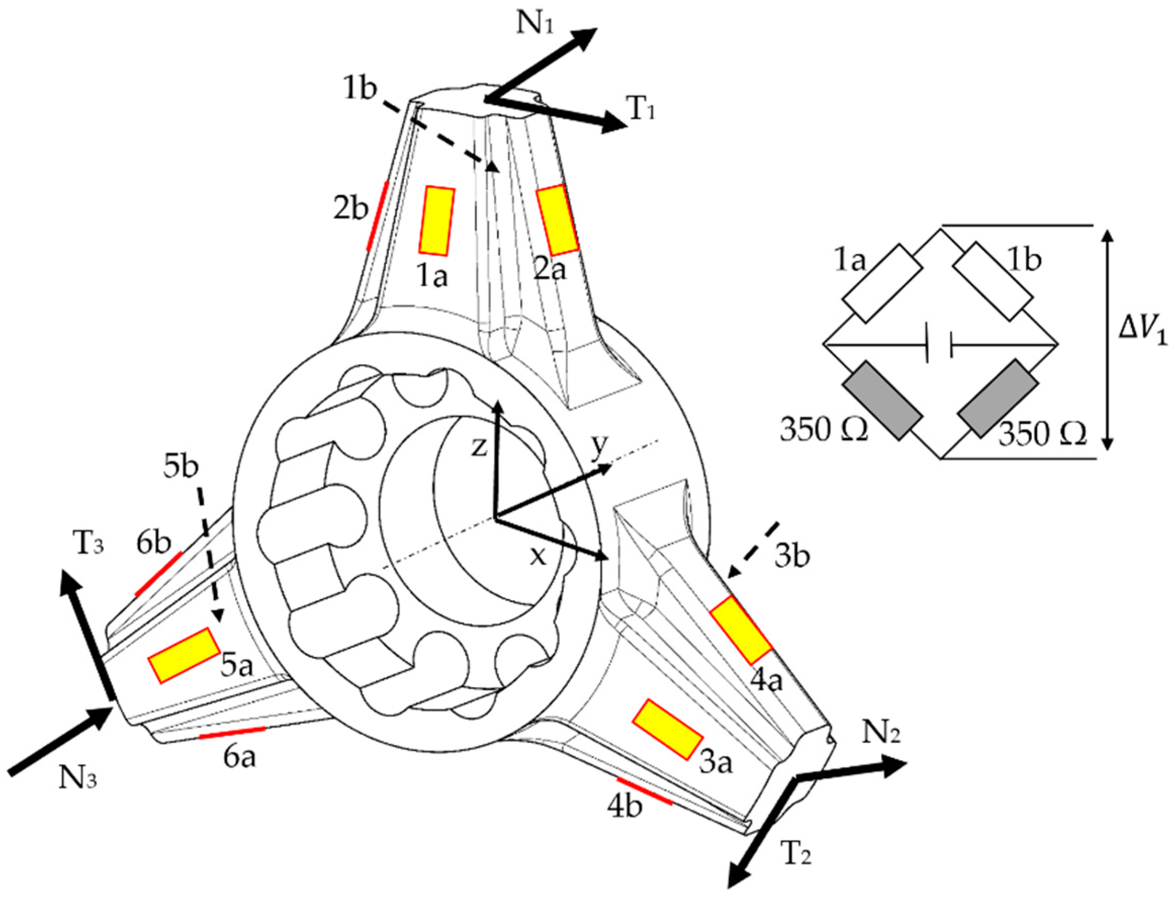
Figure 3.
Strain gauge signals and scheme of the electronic board inside the wheel rim to produce generalized force signals in the motorcycle reference system.
Figure 3.
Strain gauge signals and scheme of the electronic board inside the wheel rim to produce generalized force signals in the motorcycle reference system.
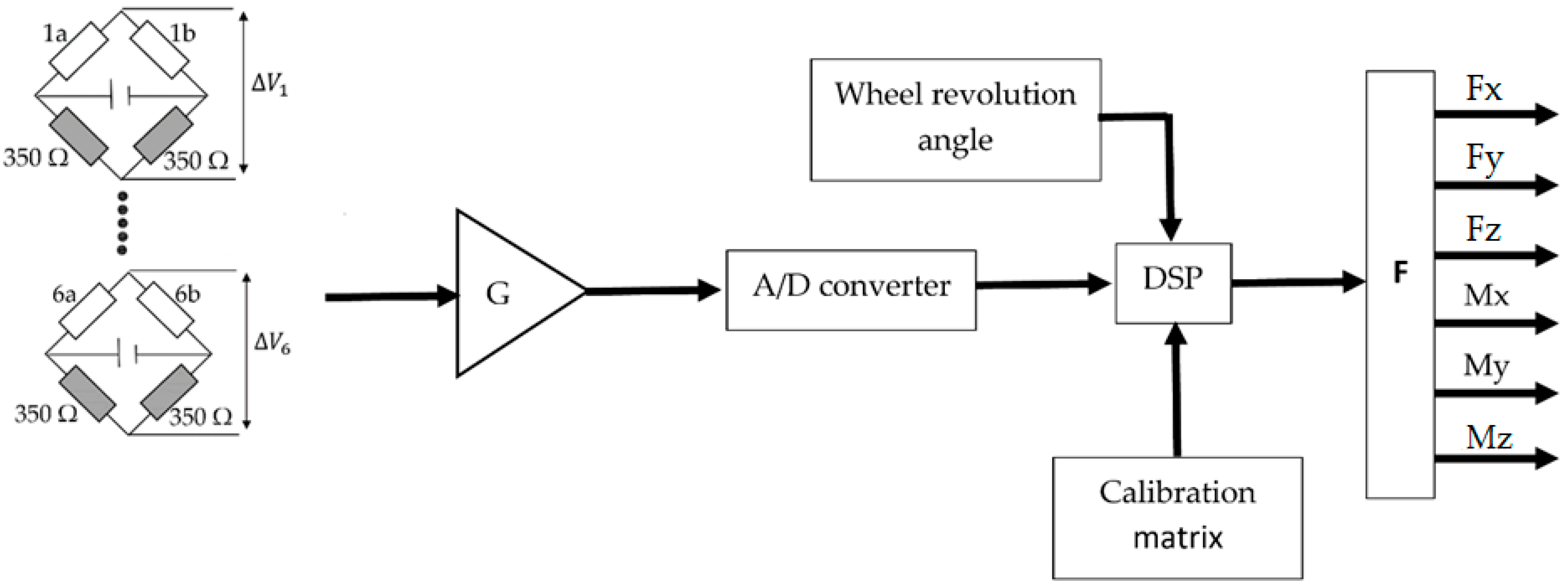
Figure 4.
Reference frames of the smart wheels.

Figure 5.
Normalized forces and moments acquired during a complete lap on circuit A by the rear smart wheel (data filtered at 10 Hz). Running conditions: #1. Pure longitudinal motion/rectilinear acceleration—green, #2. steady turning—blue #3. acceleration while cornering—magenta, #5. Gear shift—cyan.

Figure 6.
Normalized forces and moments acquired during a complete lap on circuit A by the front smart wheel (data filtered at 10 Hz). Running conditions: #1. Pure longitudinal motion/rectilinear brake—green, #2. steady turning—blue, #3. brake while cornering—magenta, #4. curb hitting—red.
Figure 6.
Normalized forces and moments acquired during a complete lap on circuit A by the front smart wheel (data filtered at 10 Hz). Running conditions: #1. Pure longitudinal motion/rectilinear brake—green, #2. steady turning—blue, #3. brake while cornering—magenta, #4. curb hitting—red.
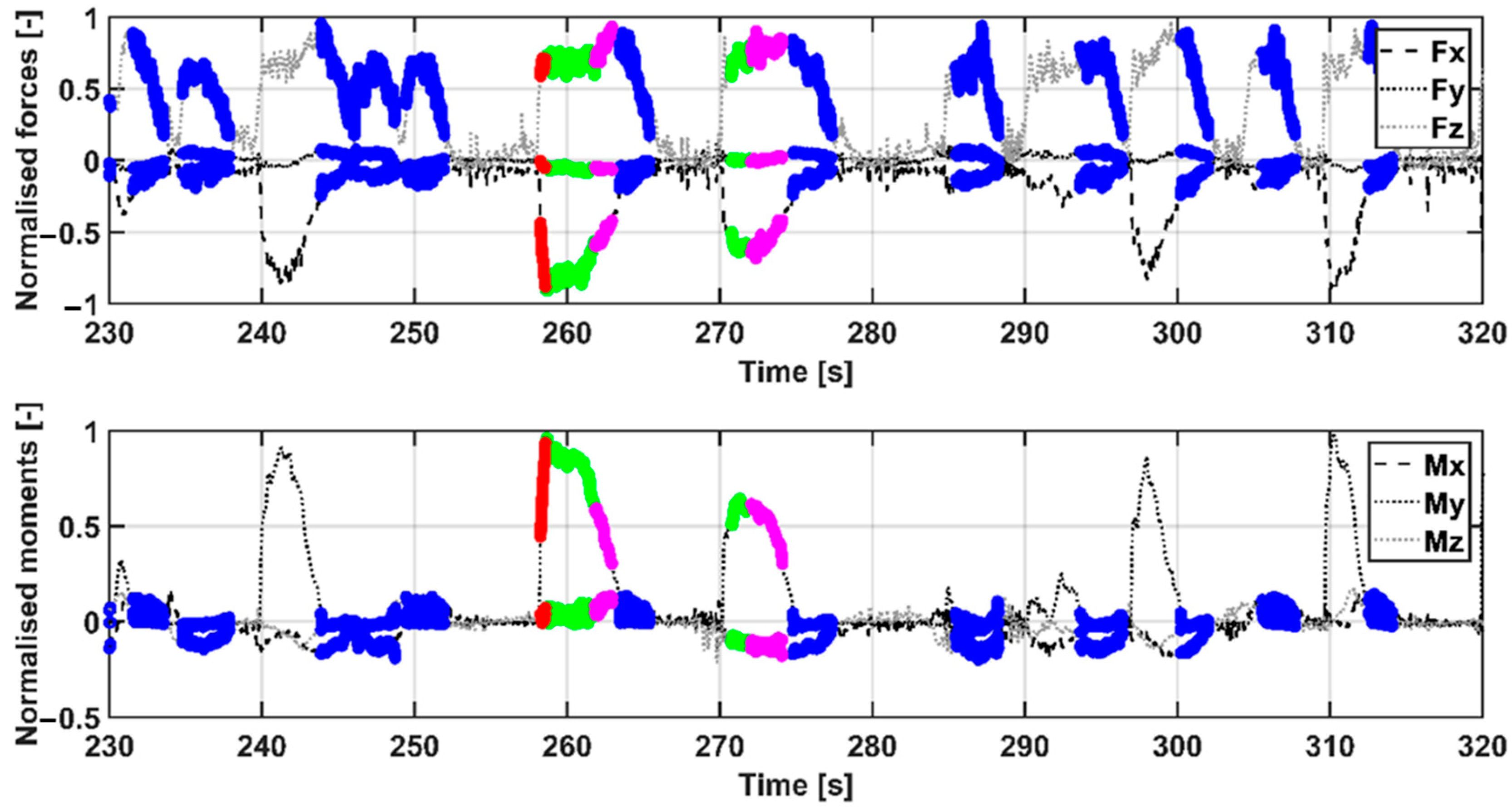
Figure 7.
Motorcycle model for pure longitudinal motion (running condition #1).

Figure 8.
Motorcycle model for steady turning (running condition #2).
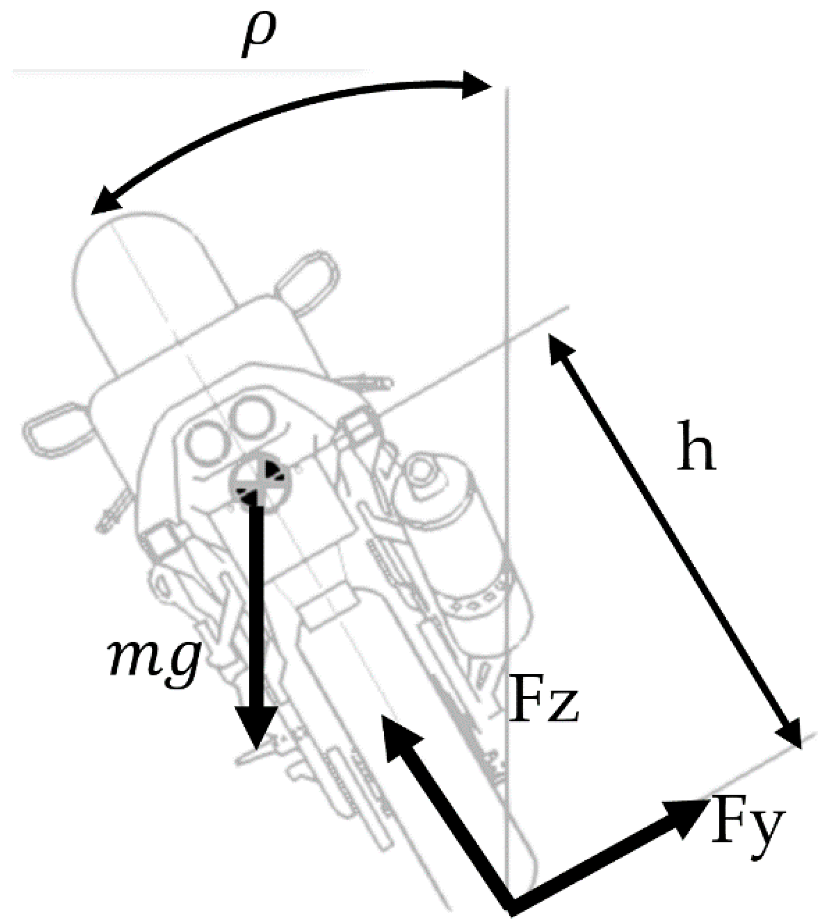
Figure 9.
Load spectrum of the measured vertical force Fz on circuit A. (a) Rear wheel. (b) Front wheel.
Figure 9.
Load spectrum of the measured vertical force Fz on circuit A. (a) Rear wheel. (b) Front wheel.
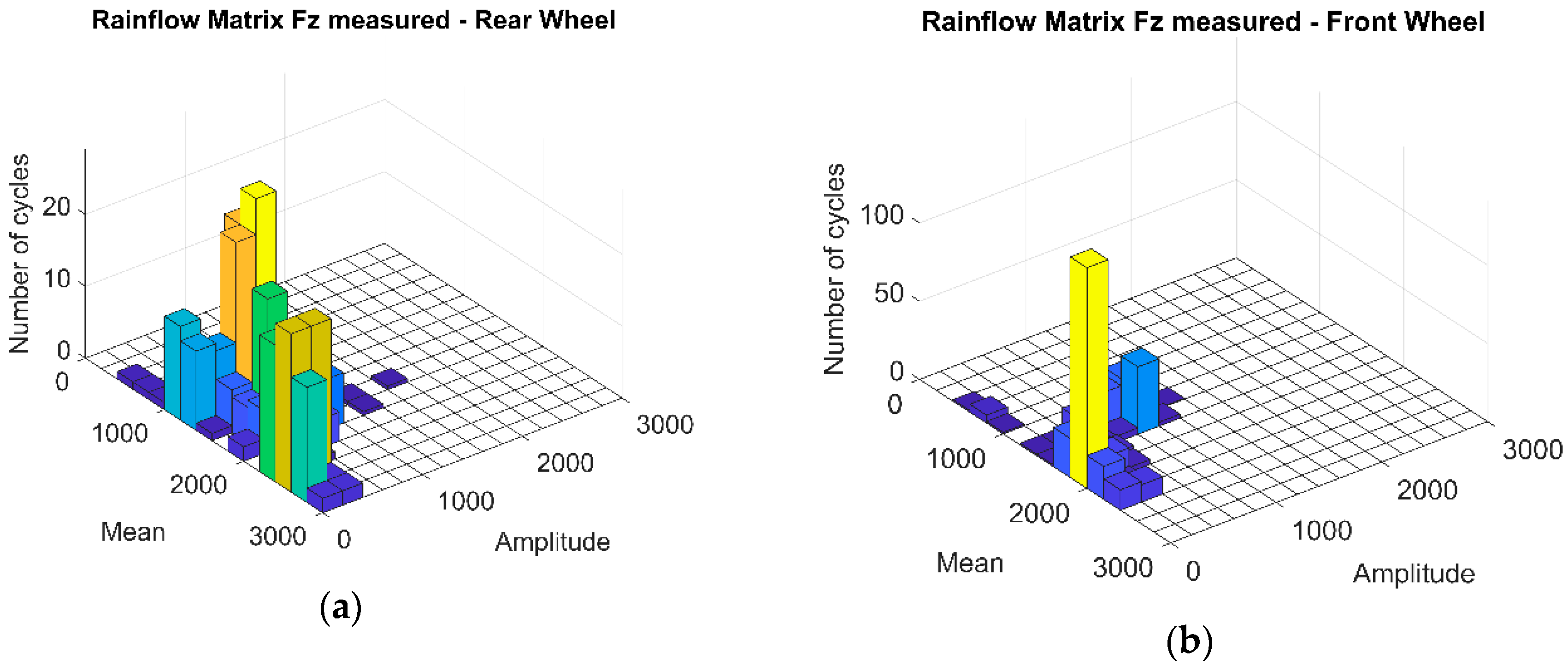
Figure 10.
Load spectrum of the longitudinal force Fx on the rear wheel on circuit A. (a) Computed by semi-analytical models (SAMs). (b) Measured.
Figure 10.
Load spectrum of the longitudinal force Fx on the rear wheel on circuit A. (a) Computed by semi-analytical models (SAMs). (b) Measured.

Figure 11.
Load spectrum of the lateral force Fy on the rear wheel on circuit A. (a) Computed by SAMs. (b) Measured.
Figure 11.
Load spectrum of the lateral force Fy on the rear wheel on circuit A. (a) Computed by SAMs. (b) Measured.

Figure 12.
Load spectrum of the moment Mx on the rear wheel on circuit A. (a) Computed by SAMs. (b) Measured.
Figure 12.
Load spectrum of the moment Mx on the rear wheel on circuit A. (a) Computed by SAMs. (b) Measured.

Figure 13.
Load spectrum of the torque My on the rear wheel on circuit A. (a) Computed by SAMs (left). (b) Measured.
Figure 13.
Load spectrum of the torque My on the rear wheel on circuit A. (a) Computed by SAMs (left). (b) Measured.
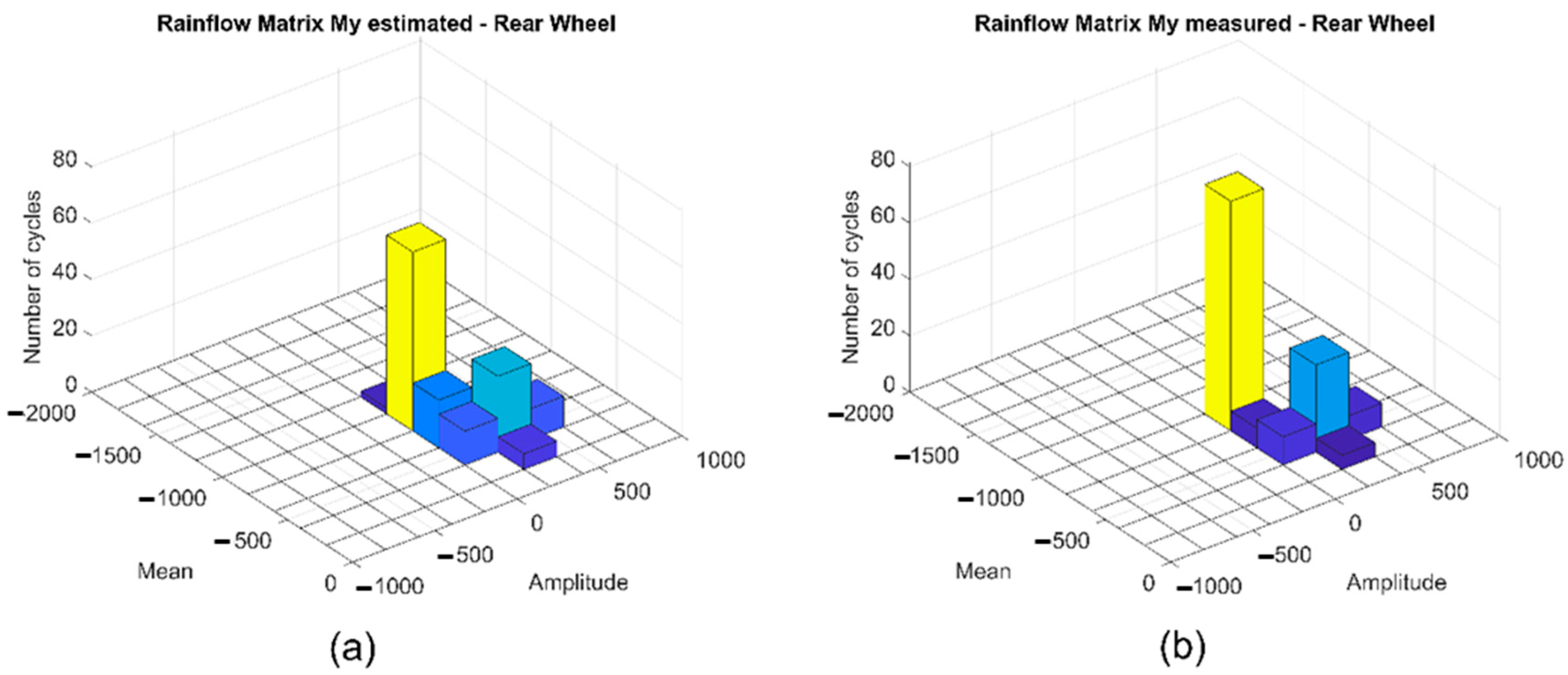
Figure 14.
Load spectrum of the longitudinal force Fx on the front wheel on circuit A. (a) Computed by SAMs. (b) Measured.
Figure 14.
Load spectrum of the longitudinal force Fx on the front wheel on circuit A. (a) Computed by SAMs. (b) Measured.

Figure 15.
Load spectrum of the lateral force Fy on the front wheel on circuit A. (a) Computed by SAMs. (b) Measured.
Figure 15.
Load spectrum of the lateral force Fy on the front wheel on circuit A. (a) Computed by SAMs. (b) Measured.

Figure 16.
Load spectrum of the moment Mx on the front wheel on circuit A. (a) Computed by SAMs. (b) Measured.
Figure 16.
Load spectrum of the moment Mx on the front wheel on circuit A. (a) Computed by SAMs. (b) Measured.
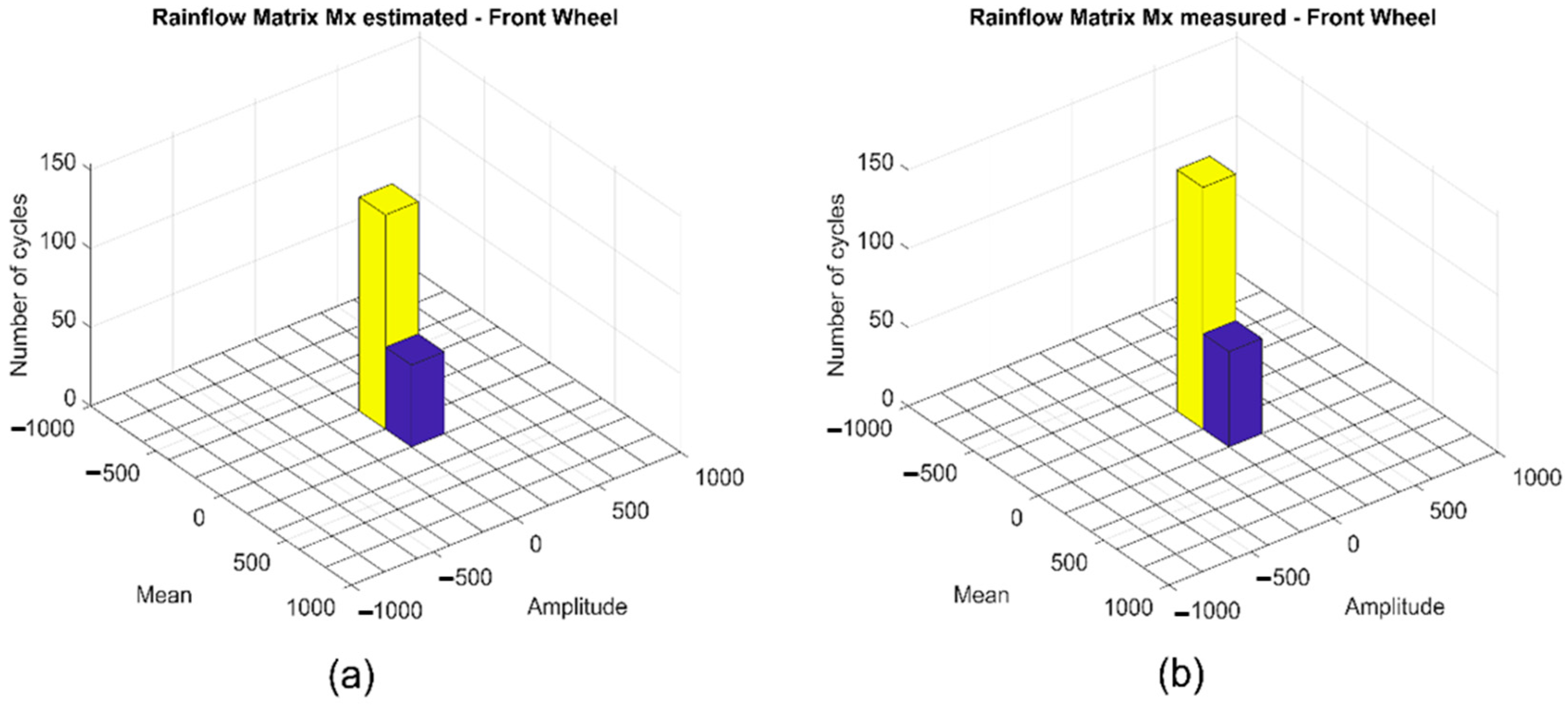
Figure 17.
Load spectrum of the torque My on the front wheel on circuit A. (a) Computed by SAMs. (b) Measured.
Figure 17.
Load spectrum of the torque My on the front wheel on circuit A. (a) Computed by SAMs. (b) Measured.
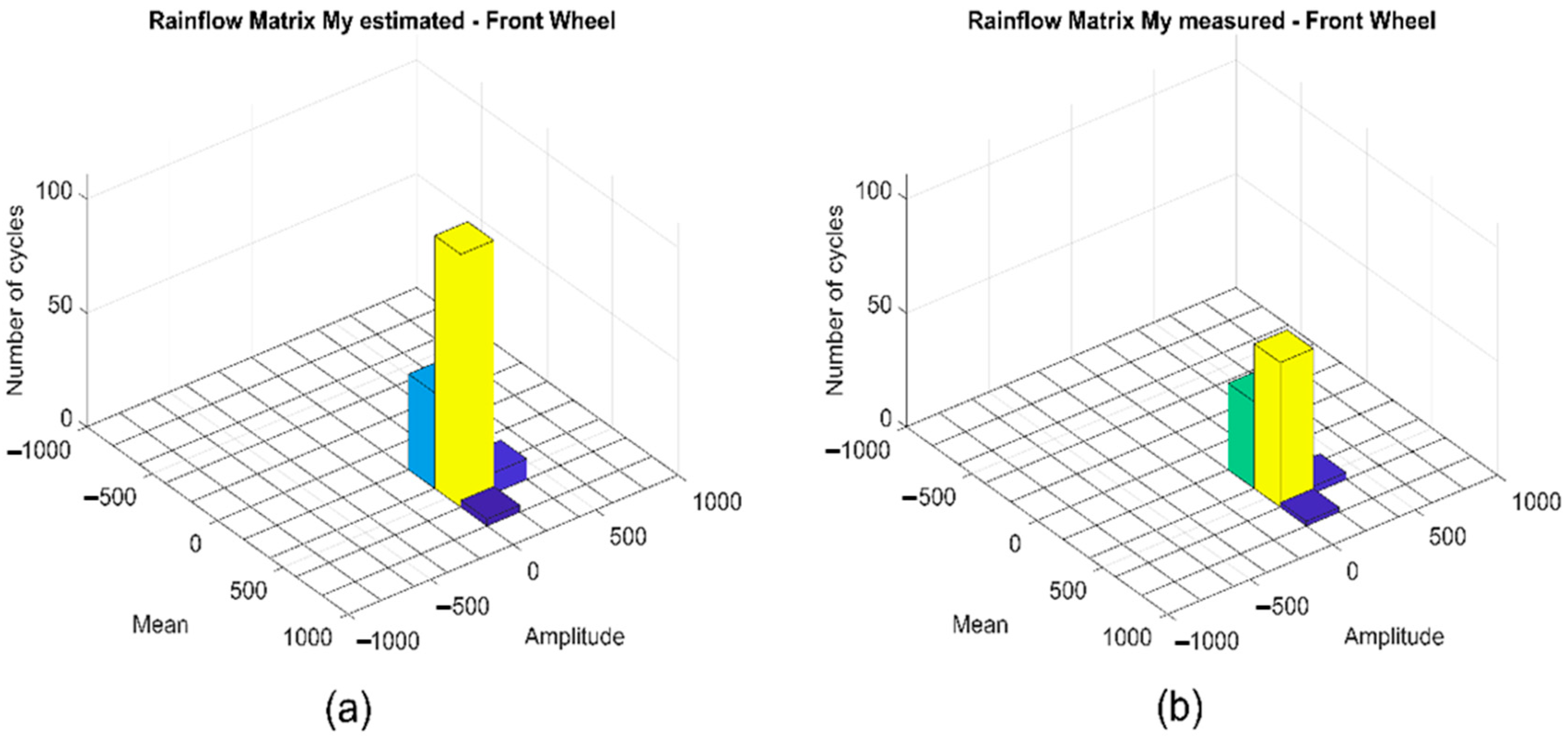
Figure 18.
Front fork main dimensions and static scheme.

Figure 19.
Maximum bending stress acting on the fork’s stems computed from the experimentally acquired forces and moments by the smart wheel (SW) during ten consecutive laps on circuit A.
Figure 19.
Maximum bending stress acting on the fork’s stems computed from the experimentally acquired forces and moments by the smart wheel (SW) during ten consecutive laps on circuit A.

Figure 20.
Load spectrum of the stress acting on the fork stems. (a) Circuit A. (b) Circuit B. Solid black line: load spectrum from experimental signals. Dashed line: load spectrum from SAMs. Grey line: Wöhler’s curve.
Figure 20.
Load spectrum of the stress acting on the fork stems. (a) Circuit A. (b) Circuit B. Solid black line: load spectrum from experimental signals. Dashed line: load spectrum from SAMs. Grey line: Wöhler’s curve.

Figure 21.
Evolution of the damage index of the front fork as function of the traveled mileage. (a) Circuit A. (b) Circuit B.
Figure 21.
Evolution of the damage index of the front fork as function of the traveled mileage. (a) Circuit A. (b) Circuit B.

Table 1.
Motorcycle characteristics.
| Physical Quantity | Symbol | Value | Units |
|---|---|---|---|
| Mass | m | 240 | kg |
| Wheelbase | p | 1.435 | m |
| Distance of the contact point from the COG | b | 0.861 | m |
| Height of the COG | h | 0.55 | m |
| Wheel radius | r | 0.3 | m |
Table 2.
Parameters for identification of driving conditions for the rear wheel.
| Pure Longitudinal (Acceleration) | Longitudinal + Cornering (Acceleration at Corner Exit) | Curb Hit |
| Tilt angle Force | Tilt angle Force | In each of the previous cases if: Interval Duration |
| Steady Turning | Gear Shift | |
| Tilt angle Force | Interval Duration | |
Table 3.
Parameters for identification of driving conditions for the front wheel.
| Pure Longitudinal (Braking) | Longitudinal + Cornering (Brake at Corner Entrance) | Curb Hit |
| Tilt angle Force | Tilt angle Force | In each of the previous cases if: Interval Duration |
| Steady state cornering | ||
| Tilt angle Force | ||
Table 4.
Geometrical parameters of the front fork.
| Parameter Description | Notation | Numerical Value | Units |
|---|---|---|---|
| Stem outer diameter | De | 43 | mm |
| Stem thickness | t | 1.5 | mm |
| Fork length | Lf | 580 | mm |
| Rake angle | β | 25 | deg |
Publisher’s Note: MDPI stays neutral with regard to jurisdictional claims in published maps and institutional affiliations. |
© 2020 by the authors. Licensee MDPI, Basel, Switzerland. This article is an open access article distributed under the terms and conditions of the Creative Commons Attribution (CC BY) license (http://creativecommons.org/licenses/by/4.0/).
Share and Cite
MDPI and ACS Style
Ballo, F.; Comolli, F.; Gobbi, M.; Mastinu, G. Motorcycle Structural Fatigue Monitoring Using Smart Wheels. Vehicles 2020, 2, 648-674. https://0-doi-org.brum.beds.ac.uk/10.3390/vehicles2040037
AMA Style
Ballo F, Comolli F, Gobbi M, Mastinu G. Motorcycle Structural Fatigue Monitoring Using Smart Wheels. Vehicles. 2020; 2(4):648-674. https://0-doi-org.brum.beds.ac.uk/10.3390/vehicles2040037
Chicago/Turabian StyleBallo, Federico, Francesco Comolli, Massimiliano Gobbi, and Giampiero Mastinu. 2020. "Motorcycle Structural Fatigue Monitoring Using Smart Wheels" Vehicles 2, no. 4: 648-674. https://0-doi-org.brum.beds.ac.uk/10.3390/vehicles2040037