
Tire Wear Reduction Based on an Extended Multibody Rear Axle Model


Chair of Dynamics and Mechatronics, Faculty of Mechanical Engineering, Paderborn University, Warburger Str. 100, 33098 Paderborn, Germany
*
Author to whom correspondence should be addressed.
Vehicles 2021, 3(2), 233-256; https://0-doi-org.brum.beds.ac.uk/10.3390/vehicles3020015
Submission received: 8 March 2021
/
Revised: 28 April 2021
/
Accepted: 29 April 2021
/
Published: 18 May 2021
(This article belongs to the Special Issue Vehicle Design Processes)
Abstract
:To analyze the influence of suspension kinematics on tire wear, detailed simulation models are required. In this study, a non-linear, flexible multibody model of a rear axle system is built up in the simulation software MSC Adams/View. The physical model comprises the suspension kinematics, compliance, and dynamics as well as the non-linear behavior of the tire using the FTire model. FTire is chosen because it has a separate tire tread model to compute the contact pressure and friction force distribution in the tire contact patch. To build up the simulation model, a large amount of data is needed. Bushings, spring, and damper characteristics are modeled based on measurements. For the structural components (e.g., control arms), reverse engineering techniques are used. The components are 3D-scanned, reworked, and included as a modal reduced finite element (FE)-model using component mode synthesis by Craig–Bampton. Finally, the suspension model is validated by comparing the simulated kinematic and compliance characteristics to experimental results. To investigate the interaction of suspension kinematics and tire wear, straight line driving events, such as acceleration, driving with constant velocity, and deceleration, are simulated with different setups of wheel suspension kinematics. The influence of the setups on the resulting friction work between tire and road is examined, and an exemplarily calculation of tire wear based on a validated FTire tire model is carried out. The results demonstrate, on the one hand, that the chosen concept of elasto-kinematic axle leads to a relatively good match with experimental results and, on the other hand, that there are significant possibilities to reduce tire wear by adjusting the suspension kinematics.
1. Introduction
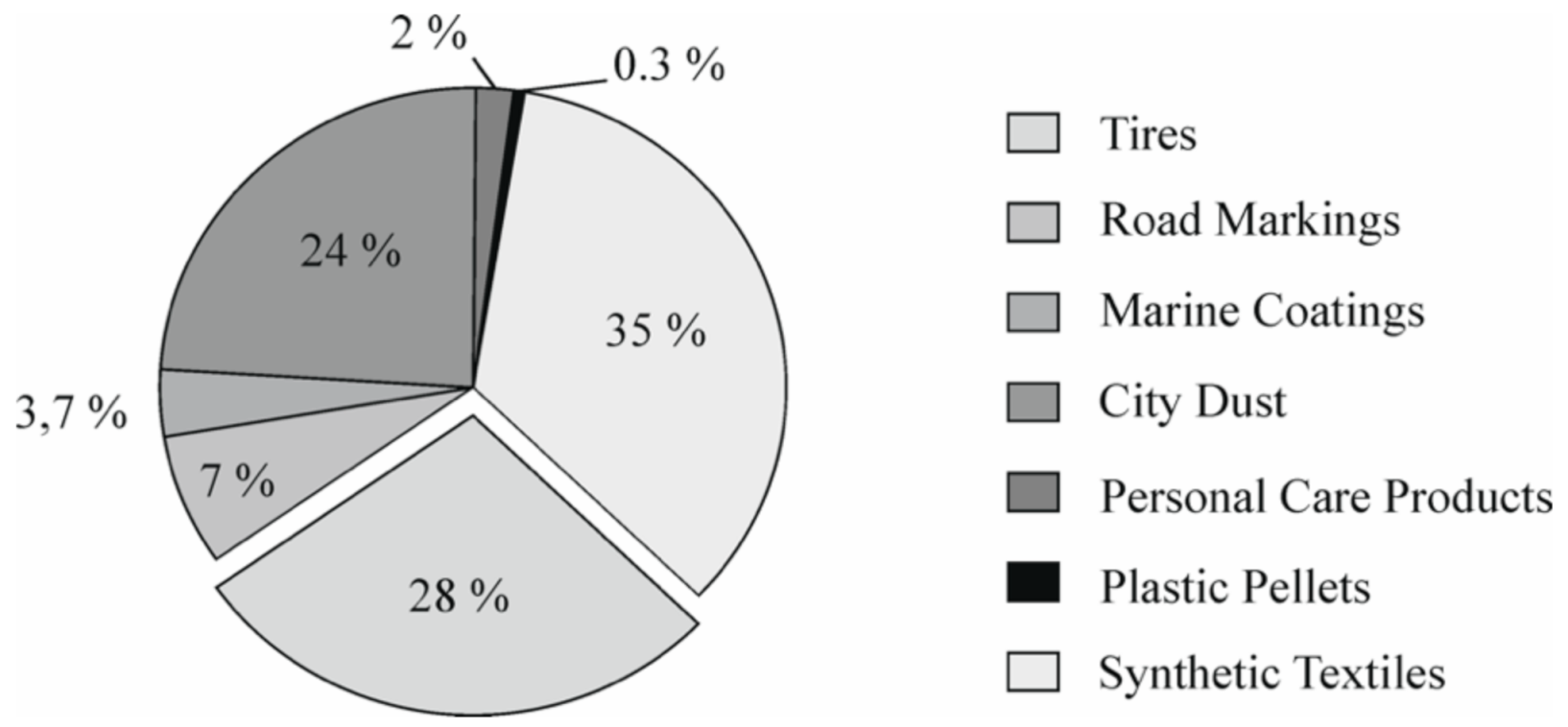
Road traffic is a key source of dust, particulate matter, CO2, NOx, and other pollutant emissions [1,2,3]. With increasing traffic, the environmental pollution caused by cars also increases. In the face of this problem, electric mobility currently moves into the focus of politics, economy, and society. Electric vehicles do not emit any kind of exhaust emissions, so environmental pollution due to the exhaust is locally reduced. However, dust or particulate matter emissions due to tire wear remain unaffected or even increase in comparison with cars with combustion engines [4,5]. To reduce the tire wear emissions of a vehicle, other concepts are needed. Tire wear is one of the main sources of microplastics, which play a major role in water body pollution [6]. In a study by Fraunhofer Institute, it was found that tire wear constitutes the major source of microplastics in Germany [7]. As evident from Figure 1, 28% of the global releases of primary microplastics to the world oceans is tire wear [6]. The amount of tire wear released while driving a car depends on many different factors such as the rubber material, environmental conditions, and driving behavior. In particular, the interaction between suspension system and wheel has a large effect on tire wear [8]. The suspension system is the connection between the vehicle body and the road. Its main task is to guide the wheel on the road and support the associated forces. Owing to road unevenness and dynamic motion, like pitch, roll, or yaw, the tire is loaded with a combined force, comprising longitudinal, lateral, and vertical forces. On the tire side, these loads are supported in an almost postcard sized contact patch (footprint) between tire and road. On the other end of the suspension, the loads are transferred to the vehicle body. The transmission of longitudinal and lateral forces is characterized by the friction between the tire tread elements and the road surface. Hence, the positioning of the tire on the road is vital [9].
Current concepts of independent suspensions consist of different linkages, which are connected to the wheel carrier on the wheel side and to the subframe on the other side. These arrangements of linkages result in a spatial wheel motion when a vertical displacement relative to the vehicle body or steering is applied. This means the wheel undergoes a motion, consisting of a translational and a rotational motion, which is defined by the number and position of the joints (kinematic points) between the suspension links [9,10,11]. These rigid-body motions are complemented by elastic deformations of structural components and rubber bushings. Elasticities change the kinematic behavior of the suspension system and, thereby, the wheel alignment, depending on operating forces and torques. These changes in wheel alignment, defined by the kinematics and compliance, are of particular importance for the driving behavior of a vehicle and the tire–road contact [9]. The spatial motion of the wheel affects the power transmission of the wheel, the friction process, and consequently the tire wear behavior owing to the relative sliding motion in the tire contact patch. Following this, the experimentally determined and calculated results presented in [12] show that it is possible to reduce tire wear by means of a new suspension concept.
To research tire wear caused by steady state or transient maneuvers, many papers dealing with analytical [13,14,15,16,17] and finite element (FE) approaches [18,19,20] have been published. The analytical wear models used are based on the physical phenomena of the wear process, considering the interaction between tire and road or test rig surface. These theoretical models can improve the understanding of relations between measurable tire state variables and tire wear. FE models are mainly used to optimize the tire itself. This includes adjustments of the structure of the tire, the tread pattern, or cross-section to obtain better tire characteristics, like a reduced wear rate or optimized stiffness. Furthermore, tire wear is often examined on test rigs at different quasi-static and dynamic loading conditions [21,22,23,24].
During the design process of a vehicle, the tire wear is usually not tested until a physical prototype is built up [12]. The tests are carried out either on real roads [13] or on a test track [25]. In the early design phase, simulation tools are commonly used to determine the effect of vehicle kinematics and forces on tire wear. In most cases, relatively simple vehicle models are used with detailed tire models, for example, FTire [26] or CDTire [27]. On the one hand, this approach neglects the complex nonlinear interactions between wheel and chassis, as explained in [12]. On the other hand, the changes in wheel alignment of a vehicle during driving are greatly affected by the elasticities of the suspension components, as mentioned above. Neglecting the interactions and elasticities of a suspension system leads to a significant deviation between prediction and reality. Tire wear depends not only on the magnitude of forces acting in the contact patch between tire and road, but also on the exact way they are generated [8,23]. This means the operating conditions of the tire should be simulated as realistically as possible [8], also considering the interactions with the subsystems suspension system and the road.
This paper presents an elasto-kinematic multibody rear axle modeling approach in MSC Adams/View, a widespread physics-based multibody simulation tool, to analyze the influence of the kinematics of wheel travel on friction work in the tire contact patch and tire wear. As a starting point, a non-steerable rear axle of a production car without any active elements is chosen. In passenger cars, many different axle concepts are present, depending on the major use case or price segment of the car [9]. In general, these concepts can be categorized into rigid axle, semi-rigid axle, and independent suspension systems. Rigid and semi-rigid axles do not have as many design possibilities as an independent suspension, so a multi-link independent suspension system is used.
The component models of the rear axle are parameterized by measurements and the resulting wheel suspension model is experimentally validated. To evaluate tire wear, two different methods are used in this study. First, under the assumption of a linear wear law according to Fleischer [28], the work done by friction in the tire contact patch is used to evaluate the tire wear. Secondly, the nonlinear wear law presented in [13,14] is used to determine the quantity and distribution of tire wear in the tire contact patch. Finally, the wheel suspension kinematics of the series axle are adjusted for the maximum reduction of tire wear during straight line driving at a constant velocity of 100 km/h. The adjustments stay inside the researched state-of-the-art of rear axle kinematics of wheel travel. The first results demonstrating the effect of toe and camber gradient adjustments at the design position on the overall work done by friction in the tire footprint have been published in [29]. The results were generated in a driving simulation with higher wheel load, which leads to approximately 20 mm positive wheel center displacement relative to the design position.
2. Rear Axle Model
As mentioned, the reference axle is a non-steerable independent rear suspension system—more precisely, an trapezoidal-link rear suspension of a production car. The modeling process is split into two main steps to guarantee verifiability at each step of the model design. At first, a multibody system model comprising only rigid bodies and ideal joints, which represent the kinematics, is built up and verified. Afterwards, the model is extended by additional rigid and elastic components to simulate elasto-kinematics and to consider all components of the axle system that influence the friction in the tire contact patch. Finally, the kinematics and compliance of the axle model are validated by comparing the simulated results to measured data.
2.1. Kinematic Model
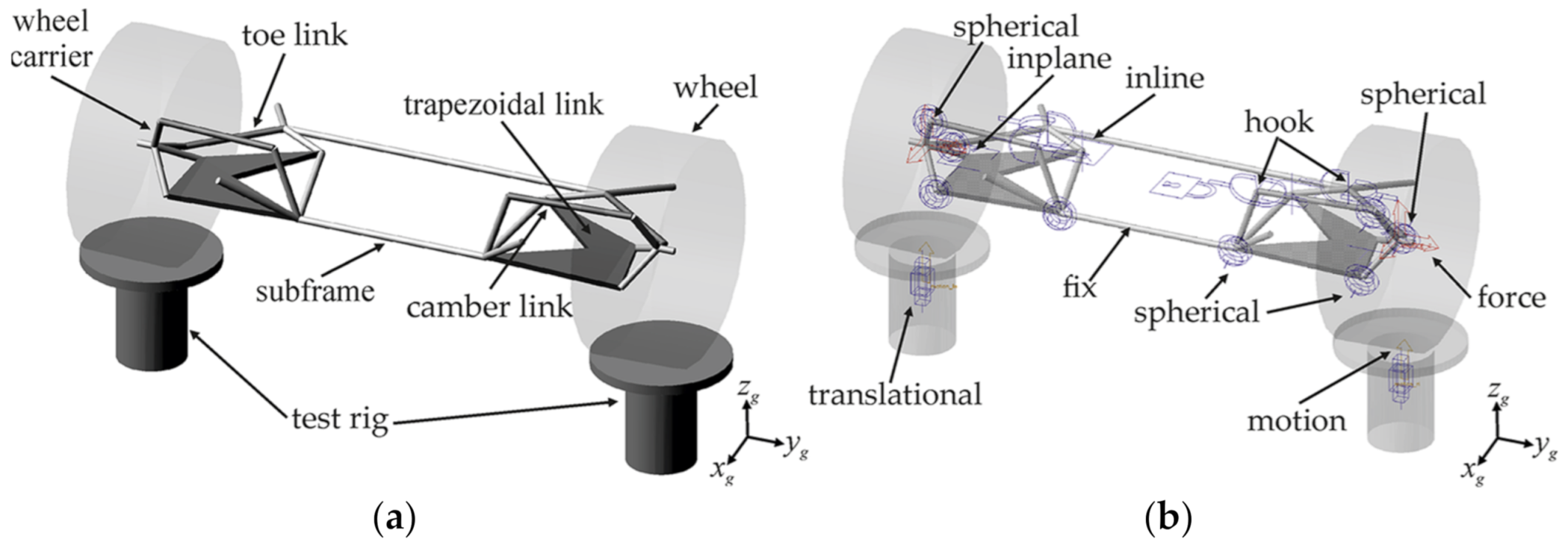
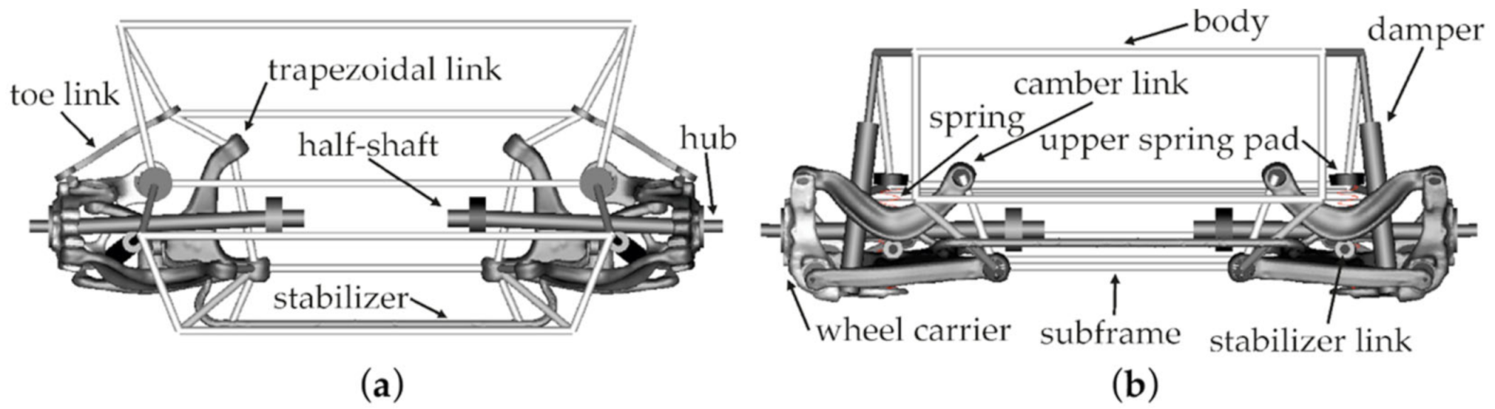
The aim of the rigid body model is to verify the modeling of the kinematics of wheel travel, so that the following improvements are based on a correct model. Most of the components (toe link, camber link, wheel carrier, and subframe) can be modeled as homogenous cylinders, as shown in Figure 2. The trapezoidal link is included as a homogenous plate. The design of the components arises from the spatial positioning of the joints (kinematic points). The kinematic model consists of eleven parts, one subframe, two toe links, two camber links, two trapezoidal links, two wheel carriers, and two wheels. The wheels have no influence on the kinematics of the suspension and, at this stage, are considered as rigid dummy parts to better illustrate the changes in wheel alignment during vertical wheel center displacement on a test rig model.
Subsequently, all parts are interconnected with joints to define the kinematics of the multibody system. For correct simulation of the kinematics of wheel travel, the correct selection of joint types is crucial. A single rigid body has six spatial degrees of freedom, three translational, and three rotational motions. By the joints, the degrees of freedom of the suspension system are reduced to two, the vertical wheel center displacement of both wheels. The number of degrees of freedom is calculated by
In the formula, is the number of rigid bodies, is the number of joints, and is the number of degrees of freedom of a specific joint [30].
The subframe is attached to the ground by a fixed joint at the center of mass of the subframe. All other joints are positioned at the kinematic points. Toe- and camber link are attached to the wheel carrier by a spherical joint and to the subframe by a hook joint. The trapezoid link is attached to the subframe and the wheel carrier with two spherical joints at both rear kinematic points. For the second connection between trapezoidal link and wheel carrier, an inplane joint is used. This joint defines a parallel plane to the -plane of the Adams ground coordinate system (. This means that the coupled points of the trapezoidal link and the wheel carrier can only move relative to each other in this plane. At the front inner side of the trapezoidal link, an inline joint is used to attach the trapezoidal link to the subframe. The inline joint only allows relative motion of the coupled bodies along a defined axis, and all rotations. The axis is oriented along the vertical direction of the Adams ground coordinate system. The wheel dummies are fixed to the wheel carrier at the wheel center. All used joints are summarized in Table 1 and shown in Figure 2.
For analysis of the kinematics of wheel travel, the axle model is extended by a test rig model. This model consists of two rigid cylinders, one for each wheel. The test rig cylinders are attached to the ground by a translational joint in vertical direction . This vertical degree of freedom is superimposed with a vertical motion, which can be defined individually for each wheel. The connections between the test rig and the wheels are realized by vertical springs between the test rig and the wheel center to lock only the vertical degree of freedom. During simulation, a translational sinusoidal motion is applied to the test rig and the wheel alignment is measured.
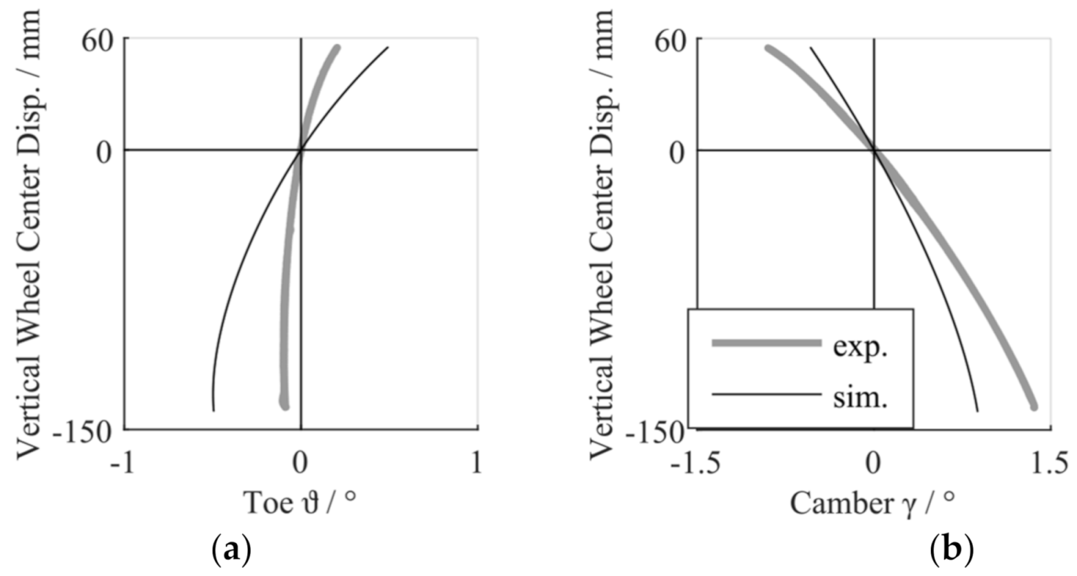
The measures of toe and camber angle and the displacement of the wheel center are implemented as described in [11]. Toe and camber angle are defined in ISO 8855 [31]. For model verification, the simulated and measured results of toe and camber angle during vertical wheel center displacement are plotted. Both curves are shown in Figure 3. The trend of both curves fits the measurements, which confirms the formal correctness of the model. At the same time, the results show that the kinematic model is not able to represent the measured kinematics of the real axle system.
2.2. Elasto-Kinematic Model
To improve the match between the model and the measurements of the kinematics, as well as to enhance the model in view of the striven investigation, the axle model is extended by several additional components. Moreover, the elasticities of the rubber metal bushings and the structural components are integrated to realize the elasto-kinematic properties of the real axle in the model. Elasto-kinematics means the displacement of the wheels relative to the vehicle body and the changes in wheel alignment caused by longitudinal and lateral forces applied at the tire footprint or wheel center [31].
2.2.1. Spring System
At first, the spring system is integrated. The spring system consists of the suspension springs with two spring pads each, the vibration dampers with bump- and rebound stops, and the stabilizer. The spring system is relevant for ride comfort, handling, and the overall safety of a car. It has to protect the occupants from impacts due to road irregularities and undesirable vertical displacement as well as pitch and roll oscillations, and maintain an even contact between tire and road [9].
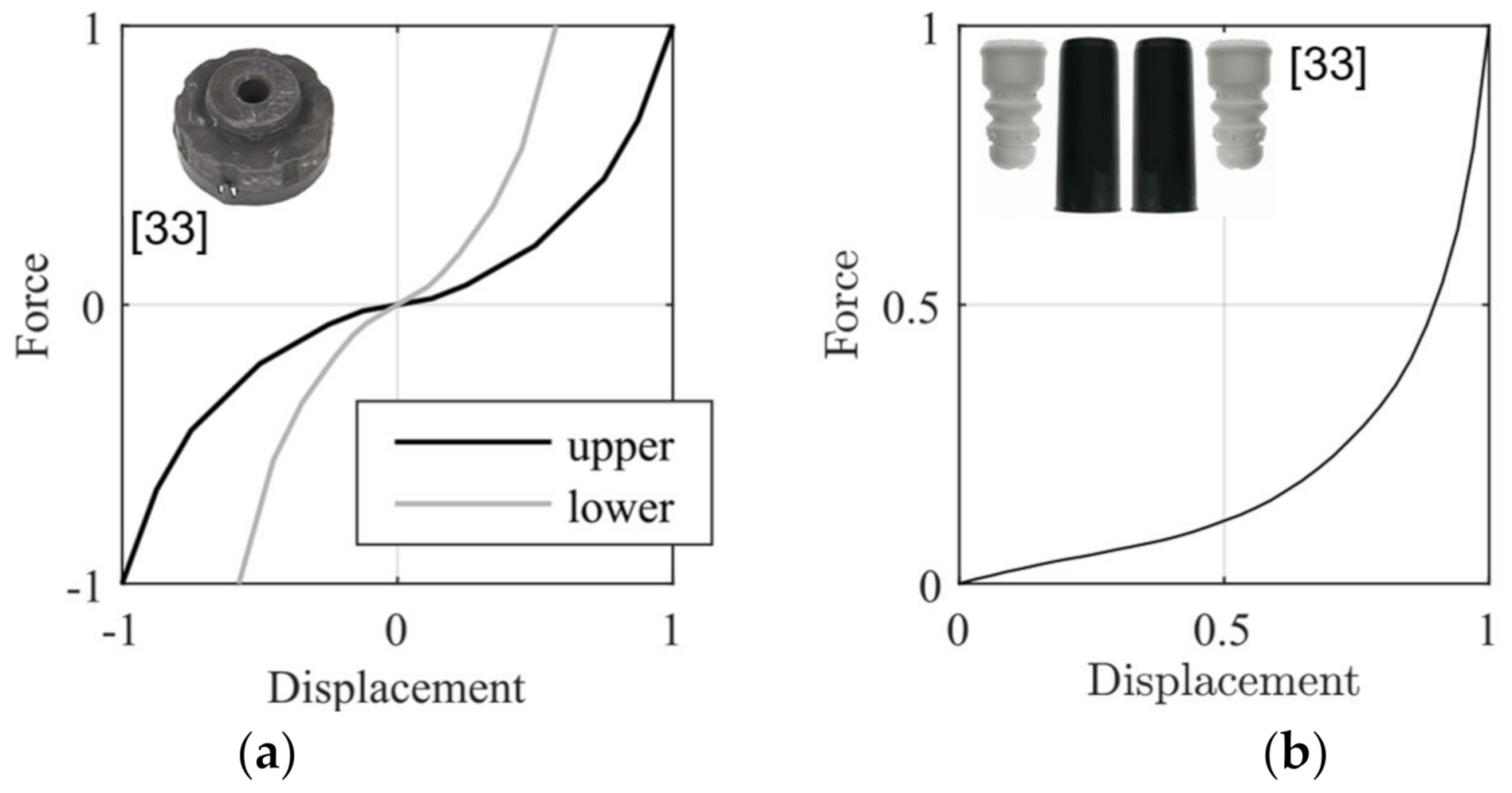
The spring of the trapezoidal rear axle is built as a coil spring and placed in front of the wheel center between two rubber spring pads, which are mounted to the vehicle body and the wheel carrier. The spring pads are modeled as a spring and damper in parallel. The spring characteristics are implemented through measured, nonlinear progressive spring characteristic curves. The normalized stiffness curve shape of both spring pads is illustrated in Figure 4a; the damping coefficient is constant in each case. The mass distribution is incorporated by rigid bodies. The coil spring can be modeled in different ways. One is to create a flexible body based on a CAD-model [12], while another way is to use a force element, as is done for the spring pads. In this study, the coil spring is modeled as a force element representing a spring with constant stiffness and no damping. The mass of the springs is represented by point masses.
In the real car, the damper is a telescopic monotube shock absorber, positioned behind the wheel center. In the axle model, the complex design of the damper is reduced to its main parts, the piston rod and main cylinder. The piston rod is mounted to the top mount, which is fixed to the vehicle body. The main cylinder is bolted to the wheel carrier by a rubber metal bushing. The piston rod and main cylinder are modeled as rigid bodies for proper mass distribution and are connected by an ideal joint. The velocity dependent damper force is nonlinear. Hence, a measured damper characteristic curve is used. The bump stop is coaxial to the piston rod and is mounted to the bottom of the top mount. It is implemented in the model as described in [11]. Its nonlinear force (Figure 4b) acts along the longitudinal direction of the damper. The rebound stop is integrated into the damper. As mentioned in [9], it is in most of the dampers. The modeling is the same as at the bump stop, but the stiffness is much more progressive. The position of the rebound stop was identified by comparing the measured overall suspension rate to the simulation results on a KnC test rig model.
A stabilizer is installed in almost every car, both at the front and the rear axle, and increases the roll stiffness without affecting the vertical spring rate [9]. When the car’s body is rolling, for example, on cornering, the stabilizer twists, which results in a restoring moment about the roll axis. The center section of the stabilizer is oriented in the lateral direction of the car and is mounted to the subframe or body by two rubber elements. The stabilizer arms point in the longitudinal direction of the car and are mounted to the suspension system by links. The coupling point of the stabilizer system and the suspension system of the reference axle is at the trapezoid link. The stabilizer links have two vulcanized bushings each, in order to connect the stabilizer to the trapezoid link. To achieve a good representation of the stabilizer system in the model, its structural components are modeled as CAD-based flexible bodies. The stabilizer is tubular, which means the wall thickness defines its stiffness. The bushings are represented as general force elements in Adams.
2.2.2. Half-Shafts
Because the chosen reference axle is a driven rear axle, the drive- or half-shafts must be integrated into the model to apply the rotational motion, which normally comes from the differential. Moreover, the half-shafts affect the kinematics of wheel travel while driving [12]. The half-shafts system consists of the wheel hub, the wheel bearing, two constant velocity joints, and the half-shaft itself. The housing of the wheel bearing is bolted to the wheel carrier, which locks its relative translational degrees of freedom. The wheel hub is pressed into the wheel bearing. In the model, the housing of the wheel bearing is attached to the wheel carrier by a rotational joint, because its translational stiffness is very high and has no impact on kinematic and elasto-kinematic characteristics of the axle, as mentioned in [32]. The torsional stiffness and damping characteristics are integrated by force elements with embedded characteristic curves. The half-shafts are linked to the wheel hub and the subframe by ideal joints, so the differential side does not move relative to the subframe and the rotational speed of the half-shaft is equal to the wheel hubs. Wheel bearing, wheel hub, and half-shaft are modeled as rigid bodies. The masses of wheel hub and wheel bearing are included in the tire model. The mass and inertia of the half-shafts are specified on the basis of a CAD model.
2.2.3. Flexible Bodies
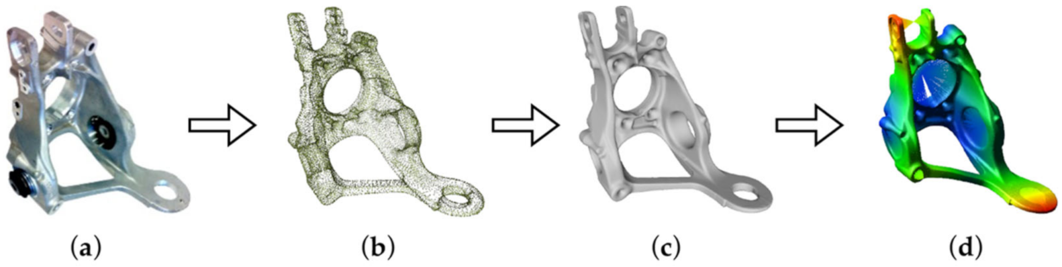
The elasticity of the structural components influences the driving behavior. As mentioned in [33], the on-load deformations of the axle components can induce displacements of the bushing positions (kinematic points) about several millimeters. This means the elasticities of the suspension links and the wheel carrier must be integrated into the model. The geometry and the properties of the material must be considered. Therefore, all suspension links and the wheel carrier are either 3D-scanned or reconstructed by SolidWorks and Catia V5. At this point, only the parts of the left wheel suspension are used to prepare CAD models, which are the basis of the flexible body models. Afterwards, the flexible body models are mirrored along the vehicle’s -plane of the ISO 8855 vehicle coordinate system. This is possible because all parts are symmetrical. Besides, it has the advantage of identical characteristics of the flexible bodies at the left and right wheel suspension. Components with complex geometries are 3D-scanned and rebuilt with the use of reverse engineering techniques and programs. The initial scan result is, in most cases, a faulty point cloud model composed of various, independent partial scans. This results in overlapping of the different meshes. Furthermore, each model contains additional errors like holes and the like, which are all remedied using the software tools Meshlab, Autodesk Meshmixer, Geomagic Control X, Materialise 3-Matic, and SolidWorks. After repair of the scan-based models, remeshing, and surface reconstruction, the suspension link and wheel carrier models are present as surface models. This step is exemplarily illustrated in Figure 5a,b.
Using SolidWorks, these models are converted into solids. The bushings are cut out, and the bearing and bushing seats and screw holes are reworked to make sure the geometry of the model resembles the real parts as closely as possible (Figure 5c). Parts with simple geometry, like the stabilizer, stabilizer link, and toe link, were redesigned directly in SolidWorks.
The prepared rigid body models are imported into Adams/View and have their material properties assigned to achieve a correct mass distribution and an accurate stiffness of flexible bodies in the model. Most of the parts are made of metal. The name of the alloy used for the aluminum parts is imprinted on their surface, so density, Young’s modulus, and Poisson’s ratio are taken from material sheets. Stabilizers are often made of 26 MnB5 or 34 MnB5 [34], so the material data of this alloy are used for the stabilizer of the model. The stabilizer links are made of glass fiber reinforced polyamide PA 6.6 GF57, which means a glass fiber ratio of 57%. The orientation of the fibers is neglected. The used properties are listed in Table 2.
Following, Adams calculates mass, center of gravity, and moments of inertia of each part. Based on these rigid bodies, flexible bodies are generated using Adams/Flex, as can be seen in Figure 5d. Adams/Flex uses the FE-solver NASTRAN to generate modal reduced FE-models by the use of the Craig–Bampton method [35]. Thereby, the degrees of freedom of any finite element model are reduced to a combination of six degrees of freedom for each attachment point, six rigid body modes, and a user defined number of normal modes. For all parts, except for the trapezoidal link, tetrahedral elements with quadratic element order are used. The trapezoidal link is a hollow body, which could not be represented by the 3D-scan based CAD-model, so quadratic shell elements with a specific thickness are used. All related kinematic points of a part are defined as interface nodes, so that forces can be applied to the flexible body models. As an attachment method, compliant RBE3 is used to add no additional stiffness to the parts. After generation of the flexible bodies, all eigenfrequencies higher than 3 kHz were disabled to reduce the simulation time. The axle model with all flexible and rigid bodies is illustrated in Figure 6. The subframe and body are assembled of cylindrical rigid bodies. Mass and inertia are supplementarily defined.
2.2.4. Bushings
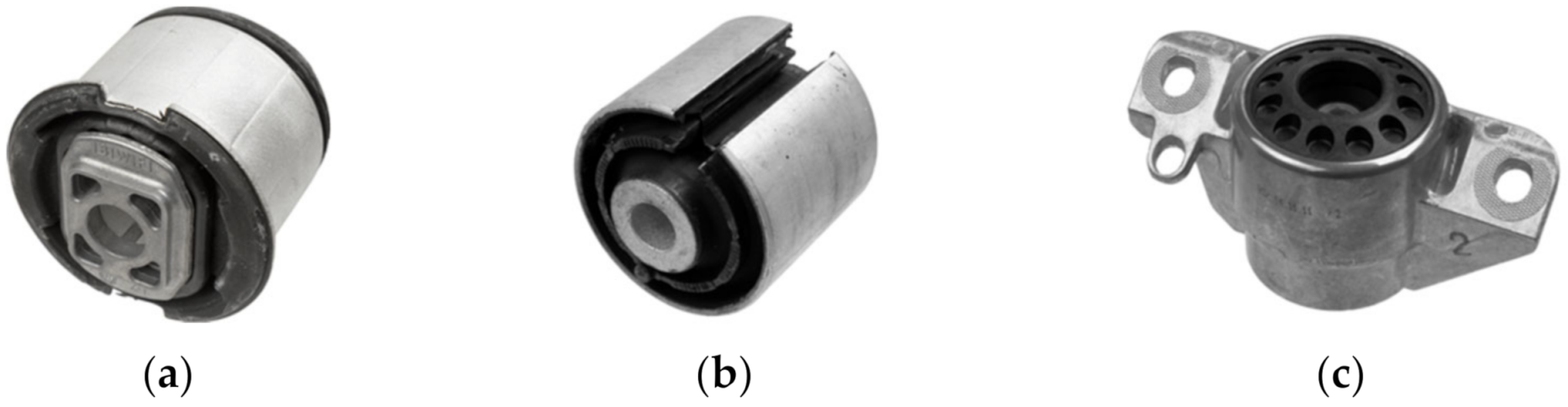
To connect the suspension parts to the reference axle, rubber metal bushings are mainly used. The properties of these elements have a huge impact on the axles’ elasto-kinematics [9,12]. Therefore, it is essential to include these parts in a detailed model. The viscoelastic behavior of a bushing is mainly defined by its material and design. There are many different bushing designs used in this rear axle. Figure 7a shows a subframe bushing, Figure 7b, a bushing with slit outer sleeve that is used more than once in the reference axle, and Figure 7c, the damper top mount to attach the damper to the vehicle body. In comparison with metallic components, rubber elements have some particularities thanks to their material properties.
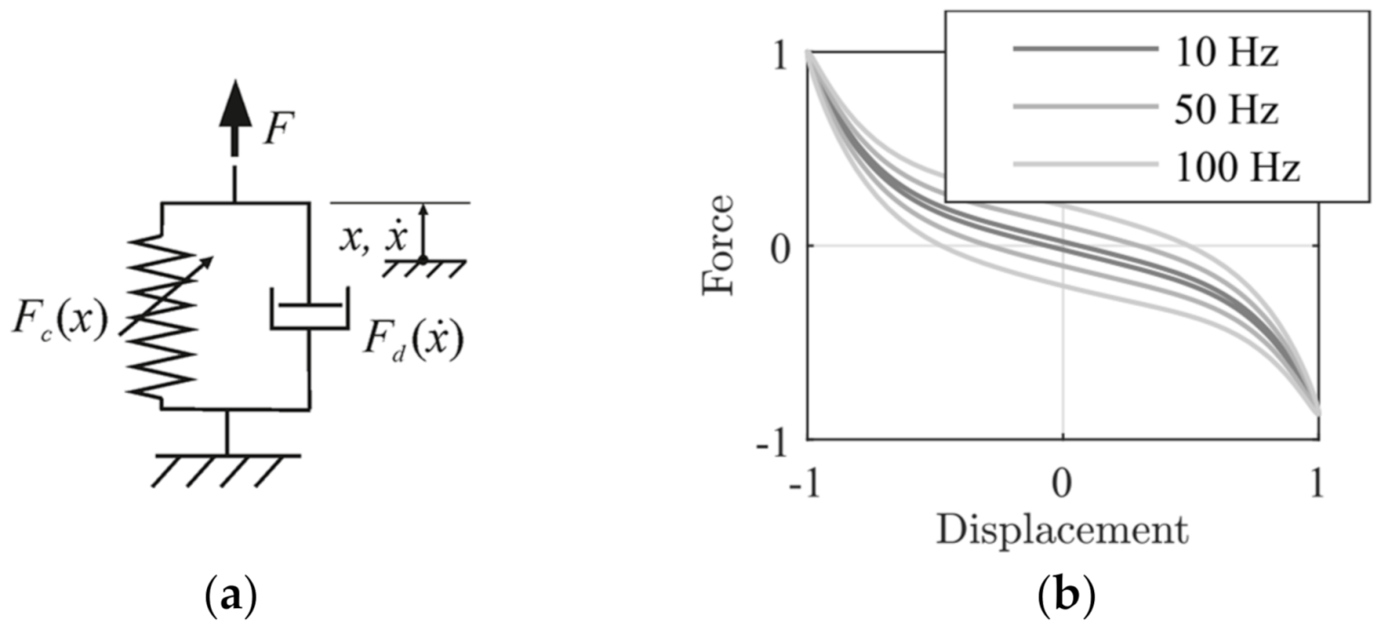
The force–displacement curve of rubber shows a hysteresis during quasi-static deformation, which means energy dissipates due to friction between molecular chains and filler particles. Moreover, the bushing stiffness depends on the excitation frequency and amplitude, which is discussed in [37] in more detail. In this study, the viscoelastic bushing properties are modeled by Kelvin–Voigt elements, which consist of a spring in parallel to a viscous damper, as shown in Figure 8a. Kelvin–Voigt models with linear springs are the standard bushing models in Adams. Instead of the standard bushing model, a general force element is used to enable nonlinear spring characteristic curves. In Adams, general force elements are freely definable six-component force elements. In Figure 8b, the resulting frequency-dependent hysteresis of Kelvin–Voigt bushing models is shown. In the case of missing measurements for individual degrees of freedom of a bushing, properties of similar bushings are used and adjusted in the later validation process.
In Adams, it is not possible to directly connect flexible bodies to each other by bushings or joints. Therefore, rigid dummy bodies are used to join the flexible wheel suspension parts. These flexible body couplings are realized at each connection of a suspension link with the wheel carrier. Where it is needed, a dummy part is attached to a kinematic point of the wheel carrier with a fixed joint. The corresponding general force element realizes the connection between the dummy part and the flexible suspension link. In total, 32 general force elements are used in this model.
2.2.5. Mass and Inertia Distribution
Owing to the driving simulations envisaged in this study, the distribution of mass and inertia features is important for realistic results as well. It is essential to model the sprung and unsprung masses because they influence the dynamics of the axle system and, as a result, the dynamics at the tire contact patch. All rotating masses, except the half-shafts, such as tire, rim, brake disc, wheel bearing, hub, and bolts, are assigned to the FTire tire model. The half-shafts’ mass and moments of inertia are defined as described before. The properties of the structural components are defined by the flexible body models. The bushings are weighed, and their mass is assigned to the dummy parts described in the previous section. The masses of the coil spring, brake caliper, and a proportional body mass are implemented as point masses. The moments of inertia of the subframe are derived from a CAD model and along with its mass assigned to the rigid body model. The body mass is attached to the almost massless rigid body chassis model, which can be seen in Figure 6. The point mass is positioned at the calculated height of vehicles’ center of gravity and in the middle of a line between both wheel centers. The height of the center of gravity of the whole vehicle is calculated by the approximation formula from [38]. The absolute value of the body mass corresponds to the loading condition and axle load distribution of the vehicle.
2.2.6. Validation of Elasto-Kinematics
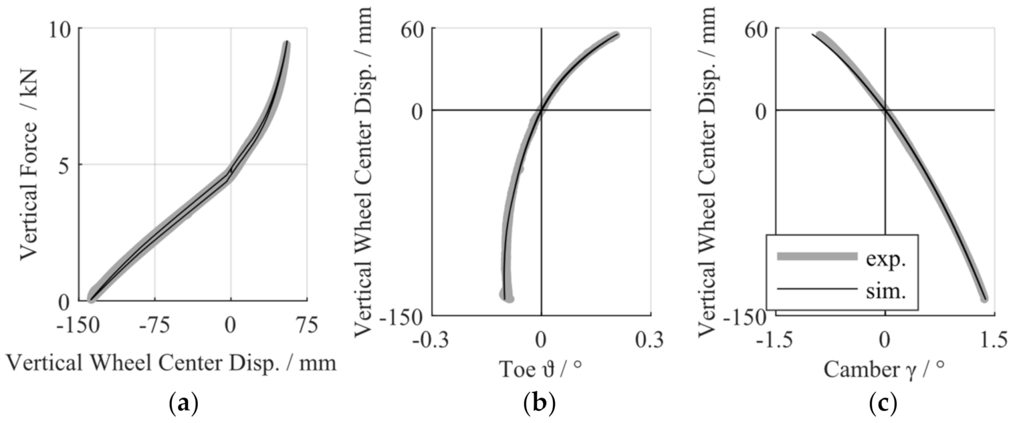
To validate the kinematics and compliance of the rear axle model, simulation results are compared to measurements, as shown in Figure 9 and Figure 10. The results are presented for the left wheel suspension only, as the graphs are also applicable to the right side because of the axles’ symmetry. To minimize the differences between the measured and simulated characteristics, finally, certain bushing parameters are adjusted. These initial deviations are normal, because measurements always underlie inaccuracies, and the properties of the rubber metal bushings scatter a lot from one another.
Figure 9 shows the validation results of vertical wheel center displacement. In all cases, zero wheel travel is defined as the design position of the axle. In Figure 9a, the overall suspension rate is plotted. Both the linear stiffness of the suspension system at negative wheel travel and progressive stiffness at positive wheel travel, which is caused by suspension spring and bump stop in series when the bump stop hits the top of the damper tube, show a good conformity. Figure 9b,c shows measured and simulated toe and camber angle change during vertical wheel center displacement. Compared with the results of the kinematic model (Figure 3), a significantly better match is achieved.
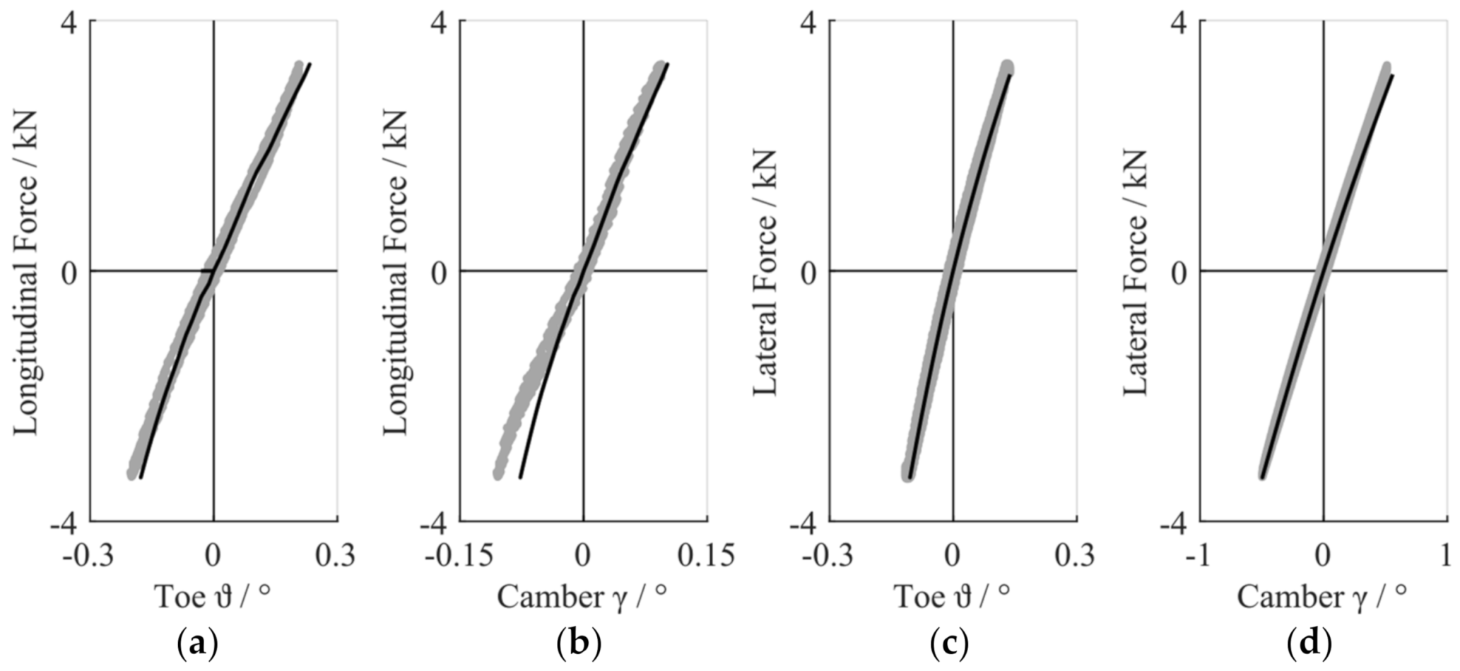
The elasto-kinematic toe and camber angle changes, specified by the compliance of the axle, are shown in Figure 10. To determine these graphs, longitudinal and lateral forces are applied isolated in the tire contact patch and the angles of wheel alignment are measured as described in [39].
A relatively good correlation between measurements and simulation results is obtained. Only the camber change caused by a lateral force in the tire contact patch deviates for negative forces around three hundredths of a degree. This could be caused by a difference in bushing stiffness or a bushing preload that is not considered in the model. However, this small deviation should not noticeably affect the simulation results.
3. Tire and Road Model
3.1. FTire Tire Model
For this study, an experimentally parameterized and validated FTire tire model is used. FTire is a fully nonlinear 3D tire structural deformation model that covers frequencies up to 250 Hz. It is capable of covering all road irregularities, even with extremely short wavelength. The model basically comprises a structural and a brush-type dynamic tread-road contact model. Additionally, there are different model extensions like a thermal model, a tread wear model, an air volume vibration model, and a flexible and viscoplastic rim model [26,40] that are not used in this study.
The structural model of the tire is based on a structural dynamics-based tire modeling approach. It defines the tire belt as an extensible and flexible ring. The tire ring consists of a finite number of so-called belt segments with mass that are coupled to the rim on one side and to their direct neighbors by nonlinear, pressure-dependent spring-damper elements. In this context, the number of belt segments defines the level of detail of the mechanical model [40]. Normally, 90 to 360 belt segments are used [41].
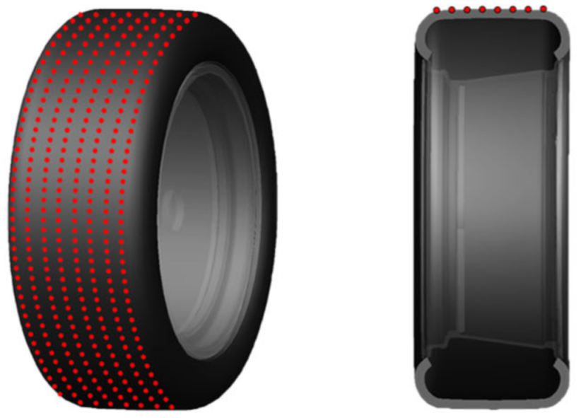
The contact between tire and road is realized by a number of mass-less contact elements (tread blocks) that are assigned to every belt segment. Usually, 5 to 50 tread blocks are used per belt segment. The tread blocks are arranged in tread strips on the tire belt. This arrangement of tread strips is exemplarily shown in Figure 11.
The tread blocks carry nonlinear spring and damper characteristics in radial, tangential, and lateral directions. On calculation of the contact forces between tire and road, FTire initially checks whether or not a tread block is in contact with the road model. For tread blocks that are in contact with the road model, first an individual contact plane and then the contact forces are calculated. More information on the FTire model is given in [40,41,42].
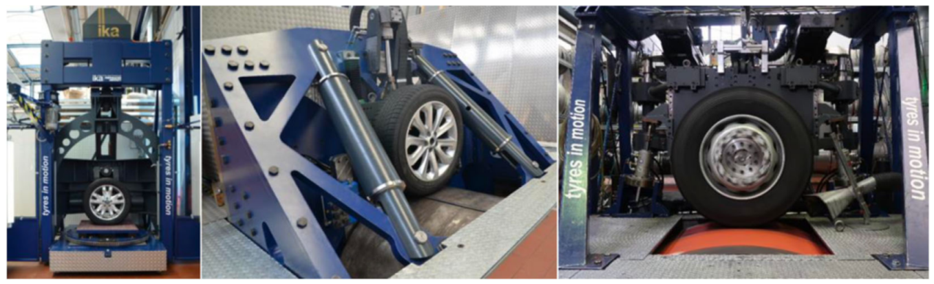
A tire of size 245/40ZR18 with an inflation pressure of 270 kPa was used. The parameterization and validation of the FTire model dataset were carried out by fka mbH Aachen, Germany for this series of tire types. For FTire modeling, several tire test rigs, as shown in Figure 12, were used, and measurements such as tire footprints, tests in static conditions, tests in steady state rolling conditions, and cleat tests were performed.
An overview of the FTire model parameters is given in Table 3. The model uses 88 belt segments with 44 tread blocks each. This results in 3872 tread blocks arranged in 22 lines (tread strips) along the tire circumference.
3.2. Road Model
In Adams, it is possible to use several different road models that are integrated into the simulation model by a road property file. In this study, two-dimensional models with stochastic road irregularities from the Adams library are used. The roughness of these road models is defined by the spectral density of the road irregularities, which results in a good accordance between the model and real road [43].
In ISO 8608 [44], road unevenness is classified into groups from A to H. Road class A is the smoothest, with very small irregularities. A road from class H is an extremely bad road, which normally cannot be found in Europe. The waviness of all road models is 2, which is a good assumption with regard to the measurements in [45].
4. Tire Wear
The total friction force in the contact patch between tire and road comprises different individual parts. These individual forces do not need to take effect simultaneously [46] and rest on physical effects, like adhesion, hysteresis, cohesion, and viscous friction [47]. The biggest contribution to rubber friction stems from adhesion and hysteresis forces. Over the years, many different empirical wear laws were developed. More information and a deeper insight in wear processes with regard to local wear of tire tread blocks can be found in [48,49].
4.1. Linear Wear Law
In the first step of this study, Fleischer’s wear law [28] is taken as a basis. This means wear is described as a result of the friction process with a proportional relation between wear volume and friction work . Using a proportionality factor , the wear can be described by
Because of this direct proportionality, the friction work is used to describe the tire wear behavior of a tire. The friction work of each contact element (FTire tread block) of the tire model is calculated based on the results of Ftire. The contact elements of the Ftire model are arranged along lines on the tire belt with uniform distance to each other. These contact elements are not observable over time, because they do not have a unique identifier. For each contact element and time step , the individual instantaneous contact forces , and sliding velocities , are calculated. With these parameters, the instantaneous power loss due to road friction of each contact element and time step is calculated by
The total instantaneous friction power in the tire footprint at time step is the sum of all contact elements:
provided that is the number of contact elements that are in contact with the road model at time step . For the calculation of the work done by friction with a constant calculation step size ,
is effective.
For evaluation of the friction work for a defined driving maneuver, the friction work for a simulation time period is defined as
In this formula, is the number of simulation steps with a constant simulation step size.
For a better comparison and presentation of the results, the friction work is normalized by the maximum of each analysis of an individual driving maneuver . The normalized friction work is referred to as .
4.2. Nonlinear Wear Law
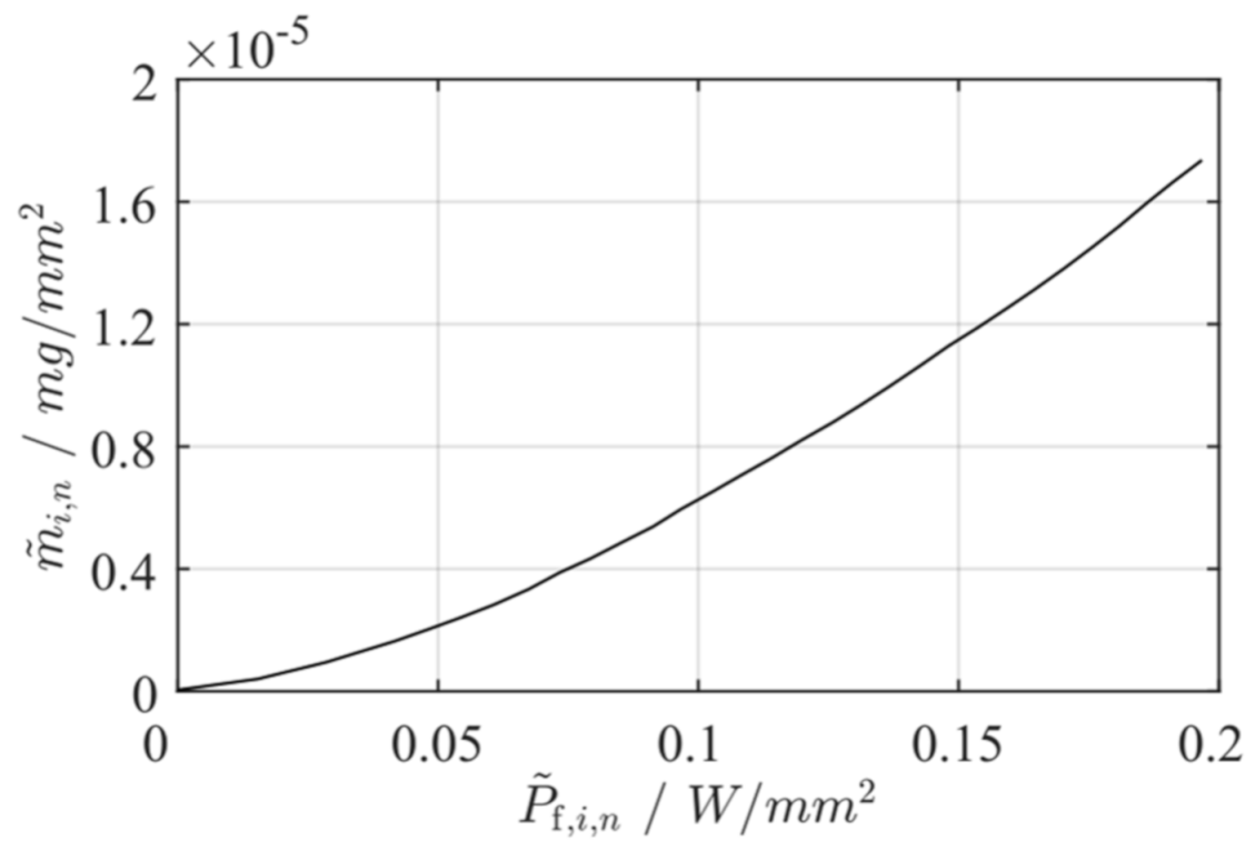
In this study, a nonlinear local tire wear law based on literature data is used to calculate the amount of tire wear generated by the rear axle simulation model. The used wear law was published in [13,14] for two different unspecified tire compounds. The local wear law is derived from experimental results at 70 °C rubber bulk temperature on an abrasive surface with an equal mean micro-texture to measured data on real road tracks. It presents the relation between power loss due to road friction per unit of contact area and mass loss per unit of contact area. This relation is plotted in Figure 13.
Therefore, the instantaneous friction power of an individual contact element at time step , calculated by the use of the FTire contact model, is divided by the present contact area of the contact element, which results in the area-specific instantaneous friction power:
5. Simulation and Results
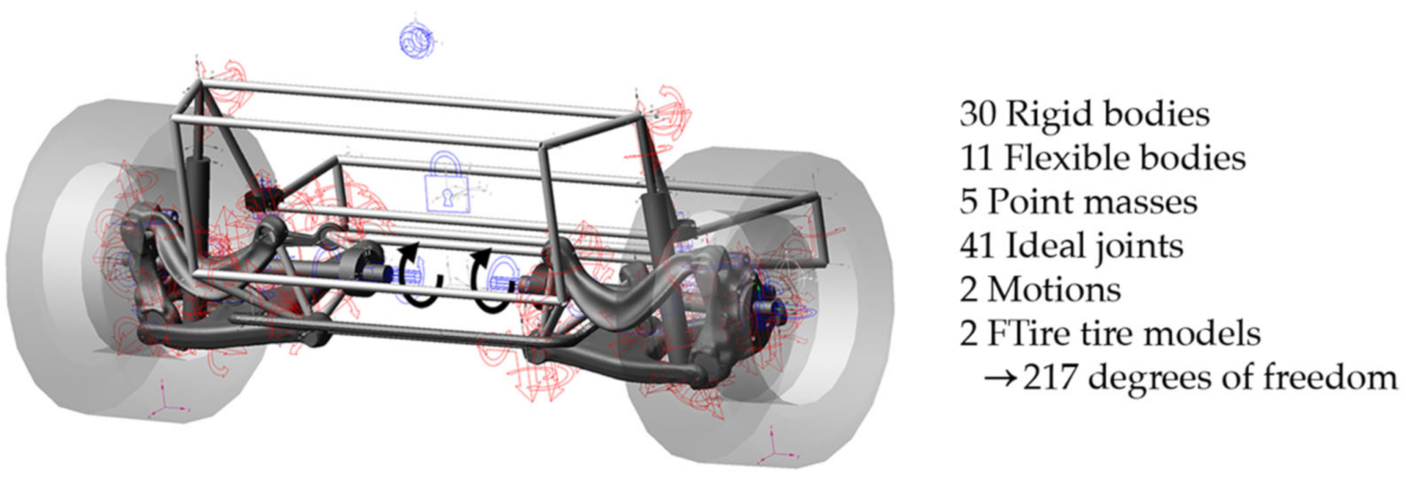
The final simulation model of the rear axle system is shown in Figure 14. It comprises 30 rigid bodies, 11 flexible bodies, 5 point masses, 41 ideal joints, 2 motions, and 2 FTire tire models, which results in 217 degrees of freedom. The rigid body part is connected to the ground to exclude pitch, yaw, and translational motion in the lateral direction.
For the simulations, a combination of three different driving maneuvers is defined. Because a single axle is being simulated, only straight-line driving events are considered. The first five seconds are the settle time of the model. After that, a rotational motion is applied to the differential side of the half shafts, as shown in Figure 14. The acceleration phase lasts ten seconds until the predefined longitudinal velocity of 100 km/h is reached. After ten seconds of driving with a constant velocity of 100 km/h, the deceleration phase begins. During deceleration, the applied rotational motion at the drive shafts is continuously reduced. The simulation model slows down within ten seconds until it stops, and the simulation ends. This velocity curve is used for all following studies. For evaluation, the driving maneuver is divided into its three load cases→.
5.1. Variation of Initial Wheel Alignment
At first, the influence of the initial toe and camber angles on the friction work in the tire footprint on a two-dimensional road model of ISO 8608 class C is analyzed. Therefore, the initial angles are varied separately, and the simulation described above is conducted. Starting at the series initial toe angle , eleven different initial toe angle settings are examined. The maximum and minimum limits are defined by
The initial camber angle is kept constant. The initial wheel alignment of each setup is listed in Table 4.
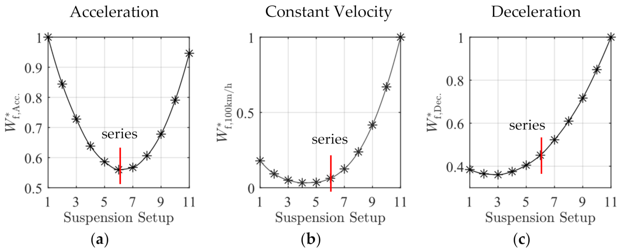
For evaluation of the influence of the different suspension setups on the total friction work in the tire contact patch, the normalized friction work is plotted as a function of suspension setups in Figure 15.
All graphs show a large influence of the initial toe angle on the total friction work of each maneuver. The initial toe angle for a minimum of friction work in the tire footprint is different for the three maneuvers. For the acceleration phase, the series angle shows a minimum. For constant driving at 100 km/h, the angle should be near to zero and more negative for deceleration.
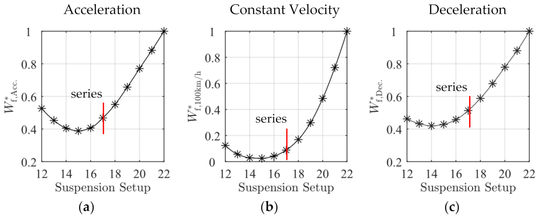
The initial camber angles are also varied. Because of the larger absolute value of the series camber angle , the angles are reduced and increased by double the absolute value, as follows:
In total, eleven suspension setups (12–22) with equal steps in camber angle variation are simulated. The initial wheel alignment of each setup is listed in Table 5.
The simulation results are shown in Figure 16. The results are again normalized by the maximum value of overall friction work of each driving maneuver and plotted as a function of the suspension setup. The initial camber angle also has a big influence on the friction work in the tire footprint. A small absolute value of initial camber angle of the axle model leads to small friction work in all examined driving events.
5.2. Variation of Kinematics of Wheel Travel
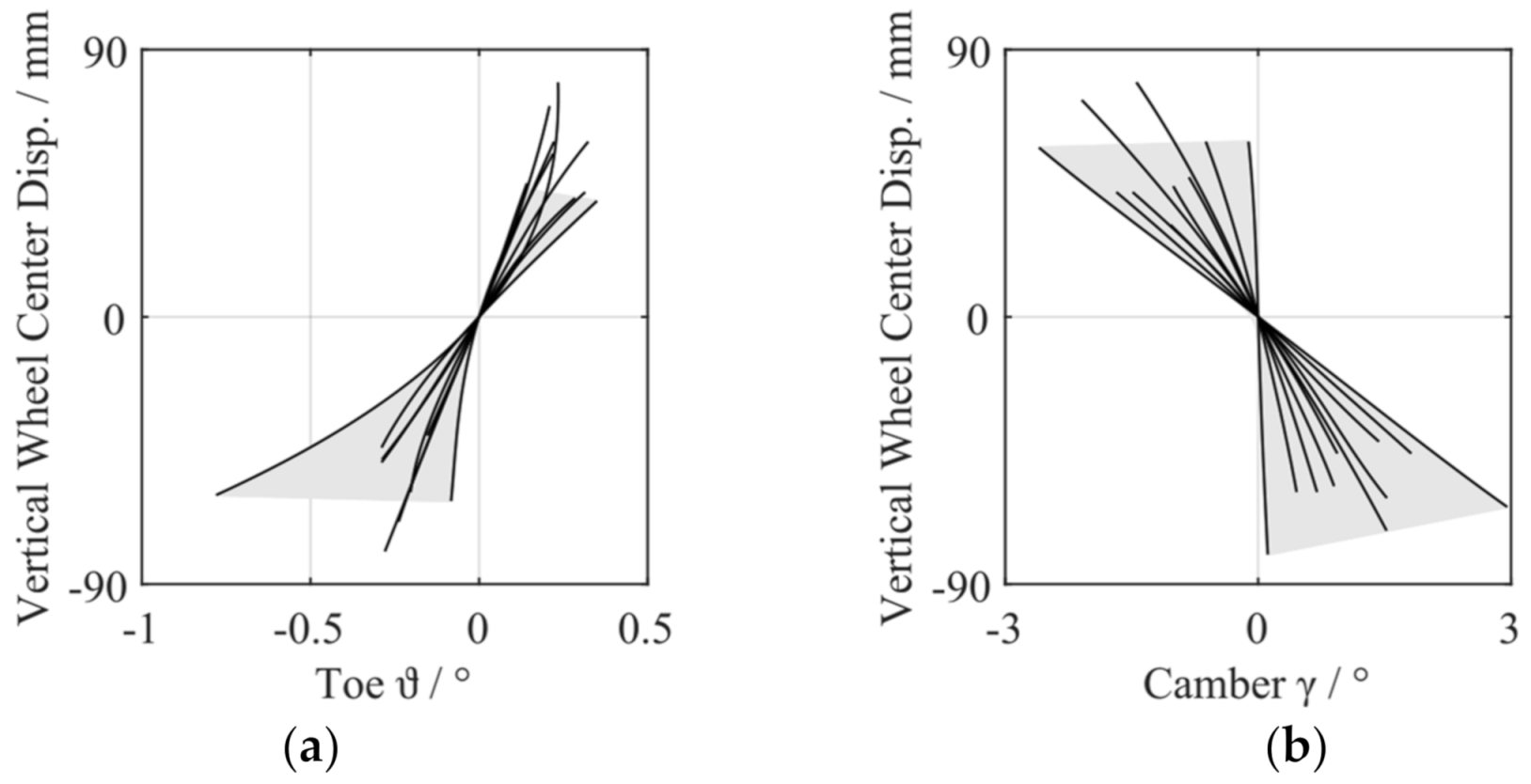
For variation of the kinematics of wheel travel, first, a research of the state-of-the-art of the kinematics of wheel travel from actual cars is carried out and presented in Figure 17. The graphs show the change in toe and camber angle during in phase vertical wheel center displacement. There is a difference in the gradient of angle change, but the trend of the curves is the same. In both graphs, no initial angle is considered.
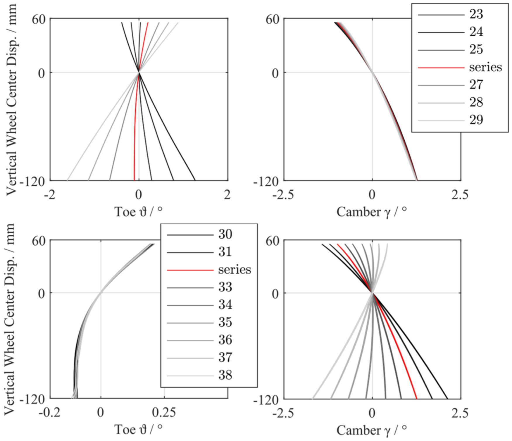
For analysis of the influence of different suspension kinematics on the friction work in the tire footprint and the tire wear, the kinematics of wheel travel of the axle model are changed [29]. The changes are conducted by adjusting the position of several kinematic points. The various resulting suspension setups with different toe and camber gradients are shown in Figure 18.
To get an isolated view of the impact of each angle gradient change, the changes are implemented separately. During variation of the toe angle gradient, the camber angle gradient stays almost the same. The same applies if the camber gradient is changed. For all simulations with these different suspension setups, the initial toe and camber angles of the production car were maintained. Because the mass of the vehicle body is not changed, the changes in suspension kinematics result in a different displacement of the wheel center relative to the vehicle body. This is compensated by adjusting the preload of the spring, so that the relative position of wheel center and body is equal for all simulations. All simulations are conducted on four different road classes defined by ISO 8608 [44], which results in 64 simulations.
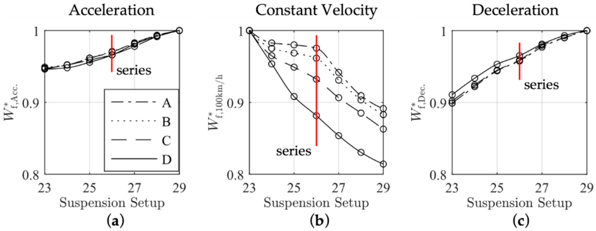
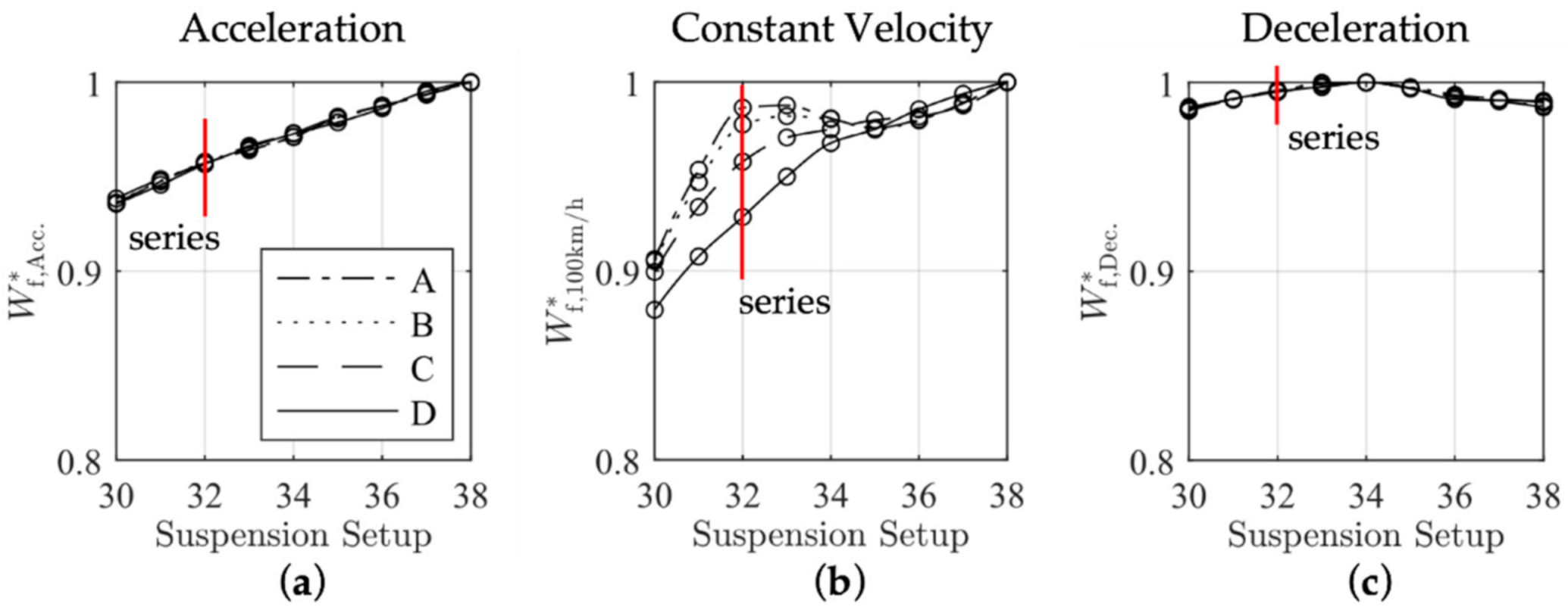
First, the influence of the kinematic toe change in combination with a negative camber gradient (setup 23–29) on the overall friction work in the contact patch between tire and road is evaluated. The simulation results for all three maneuvers are plotted in Figure 19 and Figure 20. For a better comparison, in Figure 19, the scaling of the axis is equal for all plots. In all plots, the resulting total friction work is normalized by the maximum value of friction work on each road.
The influence of the suspension setup is higher at a constant velocity than at the other maneuvers. Additionally, it is noticeable that, with a higher positive toe gradient, the friction work decreases. In contrast to the results of driving at a constant velocity, for acceleration and deceleration, a negative toe gradient seems to be better regarding friction work.
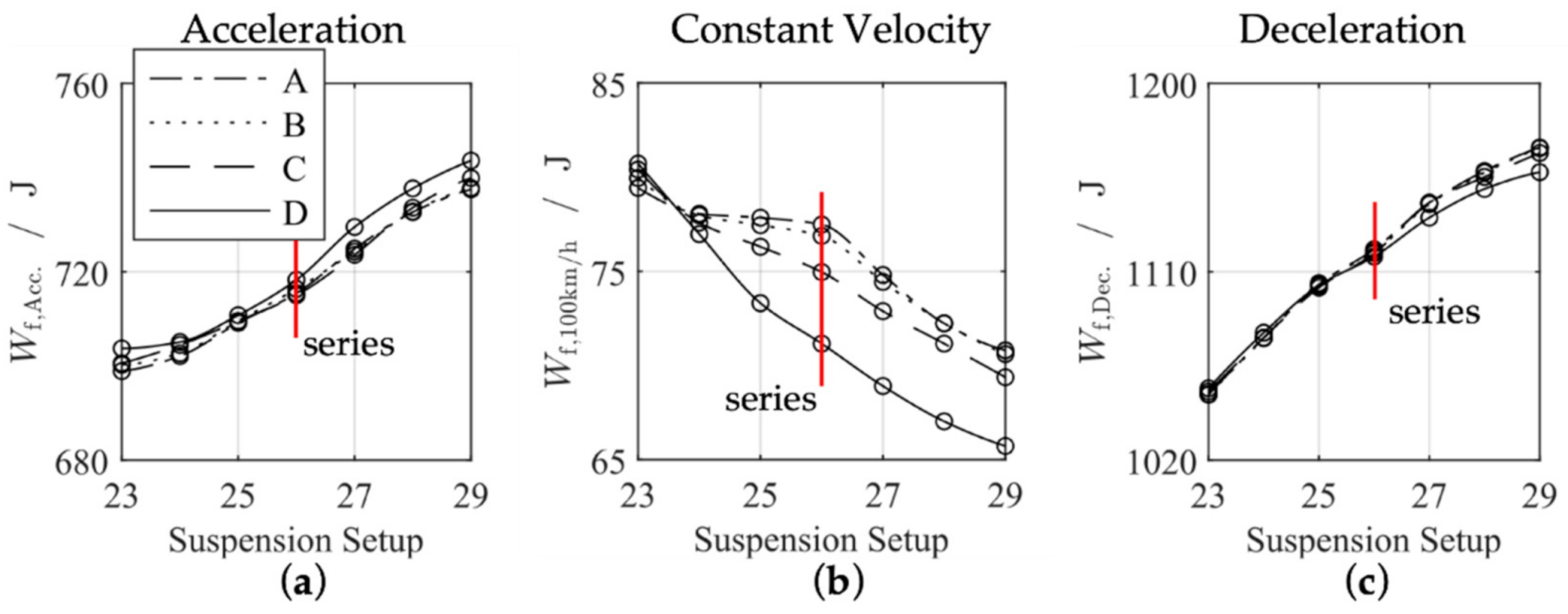
The influence of the road models with different spectral unevenness is most pronounced at the constant velocity simulation at 100 km/h. The influence at acceleration and deceleration is low. This can be explained by the different scale of the absolute values of the performed friction work in the three phases of simulation and the influence of the road (Figure 20). For constant velocity, the impact of toe gradient on the friction work increases with the unevenness of the road model starting from road class A. The amount of work done by friction significantly varies from maneuver to maneuver. The lowest friction work is done at steady state straight-line driving at 100 km/h, and the most at deceleration phase. At acceleration, the work done is almost ten times higher than at constant velocity.
Afterwards, the influence of the kinematic camber change in combination with a positive toe gradient is examined. The results are pictured in Figure 21. Again, the camber gradient produces the biggest change in friction work at a constant velocity of 100 km/h. Overall, it has to be noted that a more negative camber angle gradient in combination with a positive toe angle gradient causes a reduction of friction work in the tire footprint. During the deceleration phase, the effect is very small. The influence of the road unevenness on the results is also small during the acceleration and deceleration phases. At a constant velocity of 100 km/h, there is a significant dependence of the calculated results on the ISO 8608 road class.
For an exemplary calculation of the amount of tire wear, an average mileage of 40,000 km for a car tire is presumed. During its lifetime, a tire loses about 1 kg through wear on average [2]. The wear law used in [14] applies only to stationary operation conditions as present in the test rig. Regardless, this wear law is used as an example for an exemplary calculation of tire wear.
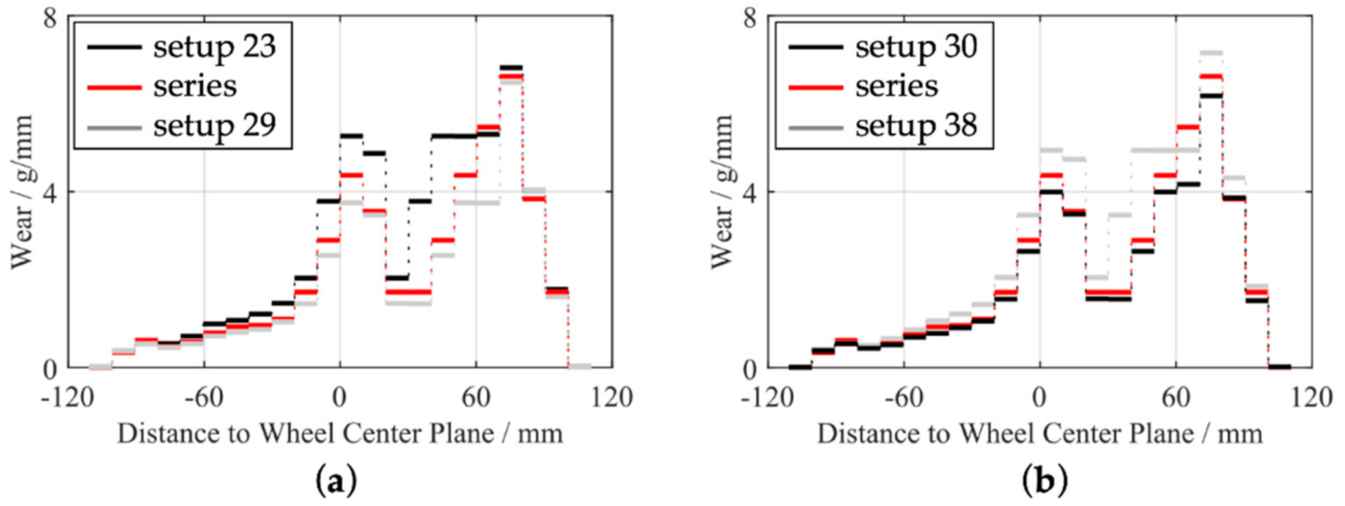
For evaluation of the saving potential, only the constant straight line driving event with 100 km/h on an ISO 8608 road model with unevenness of class C is used. The simulated results are projected to a total distance of 40,000 km to be able to make a statement regarding the lifetime of the tire. The calculation of the amount of tire wear is done with Equation (8) for all suspension setups with different kinematics (setup 23–38). In Figure 22, only the setups with minimum and maximum tire wear of the left tire are shown.
Figure 22 shows the results for two suspension setups with different toe gradients and two suspension setups with different camber gradients in comparison with the results of the series suspension setup. On the horizontal axis, the distance to the wheel center plane is used to show the tires’ lateral width. The vertical axis indicates the tire wear of each strip of the FTire contact model. The horizontal lines represent the amount of tire wear in g per mm width of the tire tread. The spatial discretization of the FTire model, described in Section 3.1, results in a tread strip width of about 10.32 mm. The total tire wear is the integral over the tire width. Both plots show more wear at the side of the tire that is oriented to the center of the vehicle. This is probably caused by the initial positive toe and negative camber angles.
Using the local wear law shown in Figure 13, suspension setup 23 leads to an increased amount of tire wear of 575 g in comparison with the series setup with 470 g. Suspension setup 29 has the highest positive toe gradient and shows the minimum tire wear. The amount of tire wear is reduced by 51 g by making the toe gradient more positive, which results in a reduction of more than 10% compared with the series suspension setup. Figure 22b shows that changing the camber gradient leads to a similar distribution of tire wear as the adapted toe gradients. With 560 g, suspension setup 38 results in the highest amount of tire wear. In comparison, suspension setup 30 results in 428 g, which means a reduction of 42 g or at least 9% compared with the series setup.
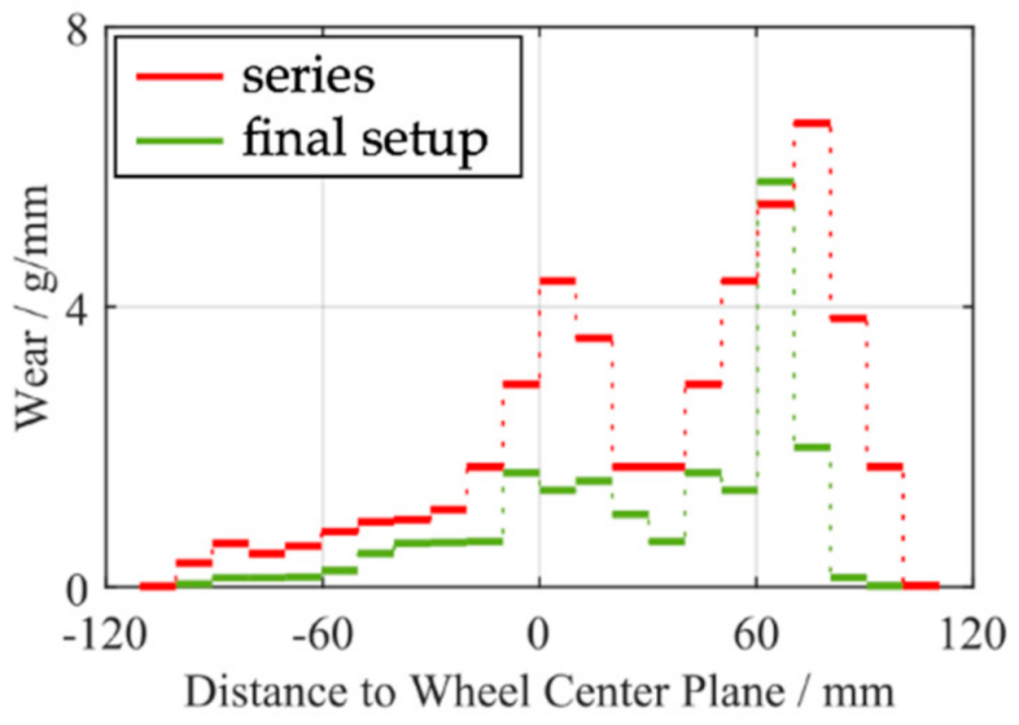
For further reduction of the tire wear during the described steady state straight line driving maneuver, both setups with the highest reduction (23 and 30) are combined, which means the toe gradient of the rear axle is changed as well as the camber gradient. This results in a significantly higher reduction of 58.1% in comparison with the series setup, which means a total tire wear of 197 g. However, the toe gradient does not fit the state-of-the-art shown in Figure 17 anymore. Therefore, the toe gradient is adjusted to the positive limit of the state-of-the-art’s toe gradients. The lateral distribution of tire wear is shown in Figure 23. With 204 g total tire wear, the produced quantity of tire wear of one wheel during a 40,000 km straight line ride with 100 km/h is reduced by 266 g (56.6%) in comparison with a wheel on a series axle.
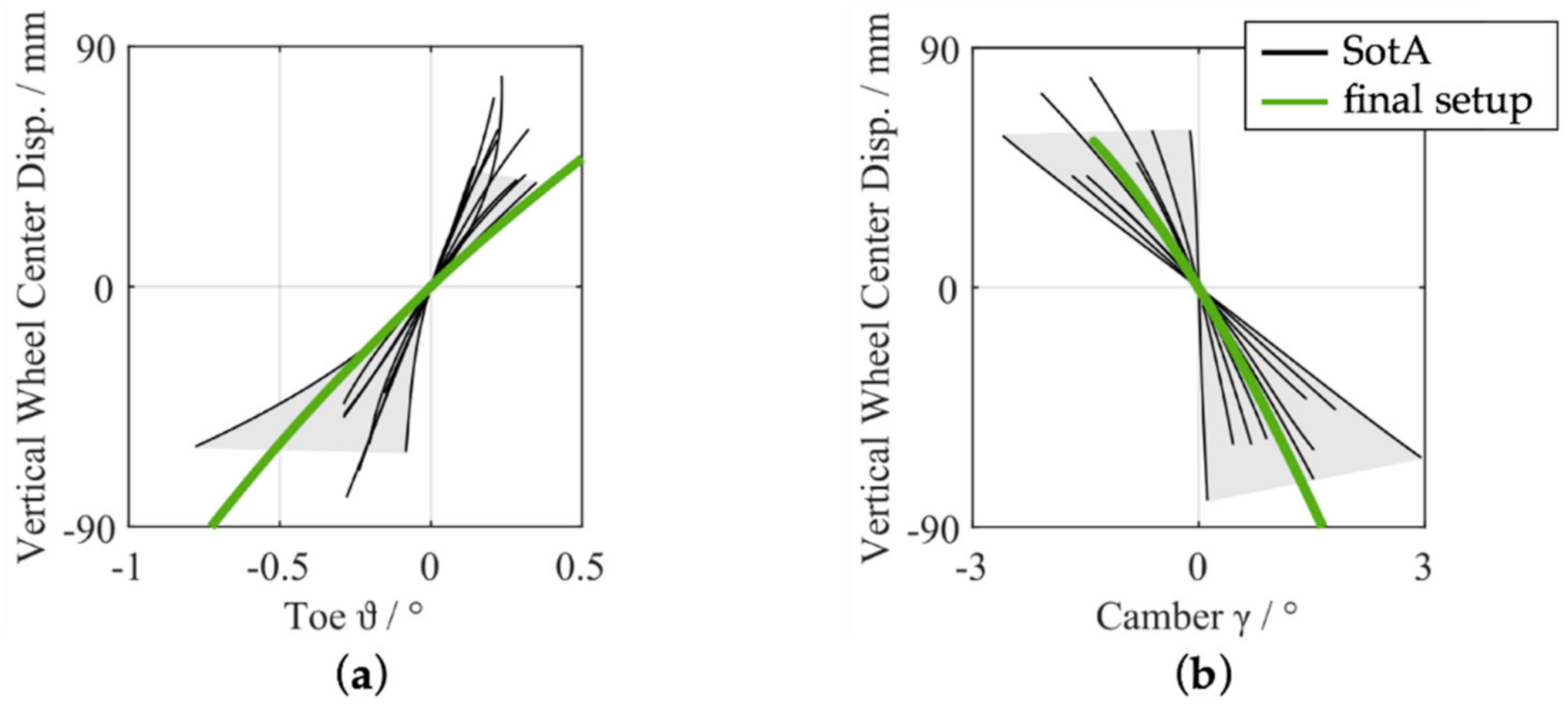
The toe and camber angle changes during vertical wheel center displacement of the adjusted suspension setup are shown in Figure 24 in comparison with the state-of-the-art from Figure 17. Both curves lie inside the spanned area of the design of the kinematics of wheel travel from actual cars. Hence, it is understood that the resulting vehicle dynamics also stays inside the merchantable range.
6. Conclusions
The results of the exemplary tire wear calculation of setups, which leads to reduction of tire wear, are listed in Table 6. Furthermore, the tire wear reduction relative to the serial setup is shown. The final and proposed setup leads to a reduction of 56.6% tire wear while straight-line driving. This means, with the new suspension setup, the tires can be used for twice as long as on the series setup. In comparison with the experimental and simulation results of [12], it can be concluded that the identified design of suspension kinematics with the lowest tire wear is completely different. However, the reduction potential identified has equal dimensions.
Based on the assumptions made and simulations done, it can be concluded that, owing to a modified suspension design process considering tire wear as the main objective, the tire wear of a car can be reduced significantly. In combination with new tire concepts with low wear, this could be a major step towards less environmental pollution.
7. Summary and Future Work
In this paper, a detailed flexible multibody simulation model of a rear axle system is built up to investigate the interactions between wheel suspension kinematics and tire wear. The modeling process was divided into two main steps, which leads to a verifiability of the model in each step. All components, which affect the dynamics in the tire contact patch, are considered, implemented, and validated on the experimental results. The elasticities of the suspension links and the wheel carrier are integrated into the model as flexible bodies. The flexible bodies are based on real geometry, derived by reengineering techniques and 3D scanning. The viscoelastic bushing characteristics are represented by Kelvin–Voigt elements with nonlinear spring stiffness. The kinematics and compliance of the final axle model are validated by measurements. For analysis of the friction process in the tire footprint while driving, the simulation model is enhanced by two experimental parameterized and validated FTire tire models and a road model with stochastic road irregularities classified by ISO 8608.
The evaluation of tire wear is conducted by the use of a linear wear law and, exemplarily, an experimentally determined nonlinear local wear law. Simulations of the three driving maneuvers, acceleration, driving with constant velocity, and deceleration, for different suspension setups were carried out. At first, the initial toe and camber angles were changed to identify their impact on the overall friction work between tire and road. The kinematics of wheel travel were changed separately, which means the toe and camber gradients were changed by adjusting the positions of kinematic points respectively without affecting each other. In this way, an isolated investigation of the influence of wheel alignment was given. Finally, the distribution of mass loss of tire tread material per unit contact width was presented for five different suspension setups for straight line driving at a constant velocity. This is the basis for a final adjustment of the suspension kinematics to achieve the largest reduction of tire wear under consideration of the compiled state-of-the-art in suspension kinematics, which leads to a significant reduction of tire wear.
It is obvious that a single axle simulation model cannot represent a vehicle as a whole. Therefore, the simulation model will be extended to a complete vehicle model. This enables pitch and yaw motion, the consideration of additional driving maneuvers like cornering or a predefined route, and a better applicability of the simulation results to the real vehicle. Especially in acceleration and deceleration, the calculated work done by friction will increase in a full vehicle simulation, because of the pitch motion, which leads to more relative motion between the wheel and chassis and, therefore, to greater changes in wheel alignment. In addition, the appropriated wear laws should be further examined.
Nevertheless, the presented results show significant potential to reduce the amount of tire wear and, in this way, environmental pollution. Up to now, this potential is not used by the automotive industry systematically. Using the proposed method, it is possible to consider tire wear as the main objective on the same level as dynamics, safety, and comfort during the design process of a suspension system.
Author Contributions
Conceptualization, methodology, validation, formal analysis, investigation, and data curation, J.S.; writing—original draft preparation, J.S.; writing—review and editing, W.S.; visualization, J.S.; supervision, W.S.; project administration, W.S.; funding acquisition, J.S. All authors have read and agreed to the published version of the manuscript.
Funding
This research was funded by Deutsche Bundesstiftung Umwelt (DBU) ![Vehicles 03 00015 i001]() .
.
 .
.Institutional Review Board Statement
Not applicable.
Informed Consent Statement
Not applicable.
Data Availability Statement
Not applicable.
Conflicts of Interest
The authors declare no conflict of interest.
References
- Diegmann, V.; Pfäfflin, F.; Wiegand, G.; Wursthorn, H. Maßnahmen Zur Reduzierung von Feinstaub Und Stickstoffdioxid; IVU Umwelt GmbH: Dessau, Germany, 2007. [Google Scholar]
- Willeke, H. CO2-Emission und Feinstaub in Verbindung mit Rollwiderstand von Reifen; DEKRA: Essen, Germany, 2008. [Google Scholar]
- Bundesministerium für Umwelt, Naturschutz und Nukleare Sicherheit (BMU). Klimaschutz in Zahlen: Fakten, Trends Und Impulse Deutscher Klimapolitik; Bundesministerium für Umwelt, Naturschutz und Nukleare Sicherheit (BMU): Berlin, Germany, 2019. [Google Scholar]
- Timmers, V.R.; Achten, P.A. Non-exhaust PM emissions from electric vehicles. Atmos. Environ. 2016, 134, 10–17. [Google Scholar] [CrossRef]
- OECD. Non-Exhaust Particulate Emissions from Road Transport; OECD: Paris, France, 2020. [Google Scholar]
- Boucher, J.; Friot, D. Primary Microplastics in the Oceans: A Global Evaluation of Sources; IUCN: Gland, Switzerland, 2017; p. 43. [Google Scholar]
- Bertling, J.; Bertling, R.; Hamann, L. Kunststoffe in Der Umwelt: Mikro- Und Makroplastik: Ursachen, Mengen, Umweltschicksale, Wirkungen, Lösungsansätze, Empfehlungen; Kurzfassung der Konsortialstudie, Fraunhofer-Institut für Umwelt-, Sicherheits- und Energietechnik; UMSICHT: Oberhausen, Germany, 2018. [Google Scholar] [CrossRef]
- Pottinger, M.G. Contact Patch (Footprint) Phenomena. In The Pneumatic Tire; National Highway Traffic Safety Administration NHTSA: Akron, OH, USA, 2006; pp. 231–285. [Google Scholar]
- Ersoy, M.; Gies, S. Fahrwerkhandbuch; J.B. Metzler: Berlin, Germany, 2017. [Google Scholar]
- Kohl, S.; Sextro, W.; Zuber, A. Benteler Vehicle Dynamics-Fahrdynamikentwicklung Basierend Auf Einer Neuen Auslegungstheorie. In 8 Tag Fahrwerks; RWTH Aachen University in Aachen: Aachen, Germany, 2012. [Google Scholar]
- Blundell, M.; Harty, D. Multibody Systems Approach to Vehicle Dynamics; Automotive Engineering Series; Elsevier Butterworth-Heinemann: Amsterdam, The Netherlands, 2004; ISBN 978-0-7506-5112-7. [Google Scholar]
- Kohl, S. Analyse Der Reibleistungsverteilung Im Reifenlatsch Unter Berücksichtigung Der Fahrwerkdynamik Eines Mehrlenkerachssystems Zur Bewertung Des Reifenverschleißes; Shaker Verlag: Aachen, Germany, 2019. [Google Scholar]
- Lupker, H.; Cheli, F.; Braghin, F.; Gelosa, E.; Keckman, A. Numerical Prediction of Car Tire Wear. Tire Sci. Technol. 2004, 32, 164–186. [Google Scholar] [CrossRef]
- Braghin, F.; Cheli, F.; Melzi, S.; Resta, F. Tyre Wear Model: Validation and Sensitivity Analysis. Meccanica 2006, 41, 143–156. [Google Scholar] [CrossRef]
- Gafvert, M.; Svendenius, J. A novel semi-empirical tyre model for combined slips. Veh. Syst. Dyn. 2005, 43, 351–384. [Google Scholar] [CrossRef]
- Sueoka, A.; Ryu, T.; Kondou, T.; Togashi, M.; Fujimoto, T. Polygonal Wear of Automobile Tire. JSME Int. J. Ser. C 1997, 40, 209–217. [Google Scholar] [CrossRef] [Green Version]
- Salminen, H. Parametrizing Tyre Wear Using a Brush Tyre Model. Ph.D. Thesis, KTH R. Institute Technology, Stockholm, Sweden, December 2014. [Google Scholar]
- Cho, J.C.; Jung, B.C. Prediction of Tread Pattern Wear by Explicit FEM. 33. J. Automob. Eng. 2014, 229, 197–213. [Google Scholar]
- Lee, S.W.; Jeong, K.M.; Kim, K.W.; Kim, J.H. Numerical Estimation of the Uneven Wear of Passenger Car Tires. World J. Eng. Technol. 2018, 6, 780–793. [Google Scholar] [CrossRef] [Green Version]
- Tong, G.; Jin, X.; Road, C. Study on the Simulation of Radial Tire Wear Characteristics. Transp. Probl. 2012, 11, 11. [Google Scholar]
- Knisley, S. A Correlation Between Rolling Tire Contact Friction Energy and Indoor Tread Wear. Tire Sci. Technol. 2002, 30, 83–99. [Google Scholar] [CrossRef]
- Sakai, H. Friction and Wear of Tire Tread Rubber. Tire Sci. Technol. 1996, 24, 252–275. [Google Scholar] [CrossRef]
- Wright, C.; Pritchett, G.L.; Kuster, R.J.; Avouris, J.D. Laboratory Tire Wear Simulation Derived from Computer Modeling of Suspension Dynamics. Tire Sci. Technol. 1991, 19, 122–141. [Google Scholar] [CrossRef]
- Stalnaker, D.; Turner, J. Vehicle and Course Characterization Process for Indoor Tire Wear Simulation. Tire Sci. Technol. 2002, 30, 100–121. [Google Scholar] [CrossRef]
- Engel, D.; Biesse, F. Simulation based tire wear prediction by vehicle and tire model coupling. In 15. Internationale VDI-Tagung Reifen-Fahrwerk-Fahrbahn; VDI-Berichte: Berlin, Germany, 2015; ISBN 978-3-18-092241-6. [Google Scholar]
- Gipser, M.; Hofmann, G.F. Tire-The Market-Leading Physics-Based Tire Model; Esslingen University of Applied Sciences: Esslingen, Germany, 2018. [Google Scholar]
- ITWM. Scalable Tire Model for Full Vehicle Simulations; CDTire: Kaiserslautern, Germany, 2017. [Google Scholar]
- Fleischer, G. Energetische Methode Der Bestimmung Des Verschleisses. Schmierungstechnik 1973, 4, 269–274. [Google Scholar]
- Schütte, J.; Sextro, W. Model-Based Investigation of the Influence of Wheel Suspension Characteristics on Tire Wear. In Proceedings of the Advances in Dynamics of Vehicles on Roads and Tracks; Klomp, M., Bruzelius, F., Nielsen, J., Hillemyr, A., Eds.; Springer International Publishing: Cham, Switzerland, 2020; pp. 1760–1770. [Google Scholar]
- Schramm, D.; Hiller, M.; Bardini, R. Modellbildung und Simulation der Dynamik von Kraftfahrzeugen; Springer: Berlin/Heidelberg, Germany, 2013; ISBN 978-3-642-33887-8. [Google Scholar]
- DIN ISO 8855:2013-11. Straßenfahrzeuge-Fahrzeugdynamik und Fahrverhalten-Begriffe; Beuth Verlag Gmbh: Berlin, Germany, 2013; p. 51. [Google Scholar]
- Trzesniowski, M. Rennwagentechnik; Vieweg, Teubner Verlag: Wiesbaden, Germany, 2012; ISBN 978-3-8348-1779-2. [Google Scholar]
- Braess, H.-H.; Seiffert, U. Vieweg Handbuch Kraftfahrzeugtechnik; Springer Vieweg: Wiesbaden, Germany, 2013; ISBN 978-3-658-01690-6. [Google Scholar]
- Salzgitter Flachstahl GmbH Borlegierte Vergütungsstähle. Available online: https://www.salzgitter-flachstahl.de/de/produkte/warmgewalzte-produkte/stahlsorten/borlegierte-verguetungsstaehle.html (accessed on 1 August 2020).
- Craig, R.R.; Bampton, M.C.C. Coupling of substructures for dynamic analyses. AIAA J. 1968, 6, 1313–1319. [Google Scholar] [CrossRef] [Green Version]
- ZF Friedrichshafen AG WebCat-Online-Katalog-ZF Friedrichshafen AG, ZF Aftermarket. Available online: https://webcat.zf.com (accessed on 2 January 2021).
- Popov, V.L. Kontaktmechanik und Reibung; Springer: Berlin/Heidelberg, Germany, 2015; ISBN 978-3-662-45974-4. [Google Scholar]
- Burckhardt, M.; Burg, H. Berechnung Und Rekonstruktion Des Bremsverhaltens von PKW; Information Ambs GmbH: Kippenheim, Germany, 1988; ISBN 978-3-88550-025-4. [Google Scholar]
- Schütte, J.; Sextro, W.; Kohl, S. Halbachsprüfstand Zur Kinematischen, Elastokinematischen Und Dynamischen Charakterisierung von Radaufhängungen. Fachtag. Mechatronik 2019, 1, 103–108. [Google Scholar]
- Cosin Scientific Software AG. F Tire-Flexible Structure Tire Model: Modelization and Parameter Specification; Cosin Scientific Software AG: Munchen, Germany, 2021. [Google Scholar]
- Gipser, M. F Tire: A Physically Based Tire Model for Handling, Ride, and Durability Part 2: Modelization. SAE Int. J. Passeng. Cars Mech. Syst. 2014, 7, 231–243. [Google Scholar]
- Cosin Scientific Software AG Cosin Scientific Software. Available online: https://www.cosin.eu (accessed on 1 July 2020).
- MSC Adams. Help—Road Models, MSC Software. 2020.
- International Organization for Standardization ISO 8608:2016-11. Mechanical Vibration Road Surface Profiles Reporting of Measured Data; International Organization Standardization: Geneva, Switzerland, 2016. [Google Scholar]
- Braun, H.; Hellenbroich, T. Messergebnisse von Strassenunebenheiten. VDI-Berichte 1991, 877, 47–80. [Google Scholar]
- Kummer, H.W. Unified Theory of Rubber and Tire Friction; B-94; Pennsylvania State Univ: University Park, PA, USA, 1966. [Google Scholar]
- Bachmann, T. Literaturrecherche Zum Reibwert Zwischen Reifen Und Fahrbahn; Berichte aus dem Fachgebiet Fahrzeugtechnik der TH Darmstadt; VDI-Verlag: Düsseldorf, Germany, 1996; ISBN 3-18-328612-2. [Google Scholar]
- Moldenhauer, P. Modellierung Und Simulation Der Dynamik Und Des Kontakts von Reifenprofilblöcken; VDI-Verlag: Düsseldorf, Germany, 2010. [Google Scholar]
- Sextro, W. Dynamical Contact Problems with Friction Models, Methods, Experiments and Applications; Springer: Berlin/Heidelberg, Germany, 2007; ISBN 978-3-540-45317-8. [Google Scholar]
- Glaser, H.; Rossié, T.; Rüger, J.; Conrad, T.; Wagner, R. Das Fahrwerk. ATZextra 2010, 15, 32–37. [Google Scholar] [CrossRef]
- Hudler, R.; Leitner, D.I.W.; Krome, H.; Steigerwald, A.; Fischer, D.I.S. Die Achsen des neuen Audi A4. ATZextra 2007, 12, 104–113. [Google Scholar] [CrossRef]
- Audi Q3: Entwicklung und Technik; Rudolph, H.-J. (Ed.) ATZ/MTZ-Typenbuch; Springer Vieweg: Wiesbaden, Germany, 2013; ISBN 978-3-658-00852-9. [Google Scholar]
- Hoffmann, J. Potentiale Einer Aktiven Achskinematik zur Optimierung des Fahrverhaltens; Schriftenreihe des Instituts für Fahrzeugtechnik, TU Braunschweig; Shaker Verlag: Aachen, Germany, 2016; ISBN 978-3-8440-4554-3. [Google Scholar]
Figure 1.
Global release of primary microplastics to the oceans according to [4].
Figure 1.
Global release of primary microplastics to the oceans according to [4].

Figure 2.
Kinematic model of the rear axle in Adams/View; (a) naming of parts and (b) positioning of the joints.
Figure 2.
Kinematic model of the rear axle in Adams/View; (a) naming of parts and (b) positioning of the joints.

Figure 3.
Comparison of experimental determined and simulated kinematics of the left wheel suspension of the kinematic model: (a) toe ϑ as a function of vertical wheel center displacement; (b) camber γ as a function of vertical wheel center displacement.
Figure 3.
Comparison of experimental determined and simulated kinematics of the left wheel suspension of the kinematic model: (a) toe ϑ as a function of vertical wheel center displacement; (b) camber γ as a function of vertical wheel center displacement.

Figure 4.
Normalized stiffness characteristic curves: (a) upper and lower spring pad; (b) bump stop.
Figure 4.
Normalized stiffness characteristic curves: (a) upper and lower spring pad; (b) bump stop.

Figure 5.
Exemplary process of flexible body creation of the left wheel carrier: (a) real part; (b) point cloud model; (c) final rigid body model; (d) flexible body model.
Figure 5.
Exemplary process of flexible body creation of the left wheel carrier: (a) real part; (b) point cloud model; (c) final rigid body model; (d) flexible body model.

Figure 6.
Axle model with flexible bodies integrated in Adams/View: (a) top view; (b) back view.

Figure 7.
Different rubber bushing designs used on reference axle system: (a) subframe bushing; (b) bushing with slit outer sleeve; (c) damper top mount [36].
Figure 7.
Different rubber bushing designs used on reference axle system: (a) subframe bushing; (b) bushing with slit outer sleeve; (c) damper top mount [36].

Figure 8.
(a) Nonlinear Kelvin–Voigt element; (b) normalized frequency dependent hysteresis of Kelvin–Voigt element, simulated for 10, 50, and 100 Hz.
Figure 8.
(a) Nonlinear Kelvin–Voigt element; (b) normalized frequency dependent hysteresis of Kelvin–Voigt element, simulated for 10, 50, and 100 Hz.

Figure 9.
Comparison of experimental determined and simulated kinematics of the left wheel suspension of the elasto-kinematic model: (a) vertical wheel center displacement as a function of vertical force; (b) toe ϑ as a function of vertical wheel center displacement; (c) camber γ as a function of vertical wheel center displacement.

Figure 10.
Comparison of experimentally determined and simulated elasto-kinematics of the elasto-kinematic model of the left wheel suspension: (a) toe ϑ as a function of longitudinal force; (b) camber γ as a function of longitudinal force; (c) toe ϑ as a function of lateral force; (d) camber γ as a function of lateral force.

Figure 11.
Example illustration of the arrangement of brush-type contact elements (tread blocks) in lines (tread strips) on the tire belt of the FTire model.
Figure 11.
Example illustration of the arrangement of brush-type contact elements (tread blocks) in lines (tread strips) on the tire belt of the FTire model.

Figure 12.
Tire test rigs used for experimental investigation of tire properties to parameterize and validate the FTire tire model.
Figure 12.
Tire test rigs used for experimental investigation of tire properties to parameterize and validate the FTire tire model.

Figure 13.
Local wear law of a tire tread compound at 70 °C rubber bulk temperature and a surface micro-texture having a mean wavelength of according to [14].
Figure 13.
Local wear law of a tire tread compound at 70 °C rubber bulk temperature and a surface micro-texture having a mean wavelength of according to [14].

Figure 14.
Final simulation model of the rear axle system in Adams/View.

Figure 15.
Normalized friction work in the tire contact patch as a function of suspension setup (1–11) for three different straight-line driving maneuvers on a two-dimensional road model of ISO 8608 class C: (a) Acceleration; (b) Constant Velocity; (c) Deceleration.
Figure 15.
Normalized friction work in the tire contact patch as a function of suspension setup (1–11) for three different straight-line driving maneuvers on a two-dimensional road model of ISO 8608 class C: (a) Acceleration; (b) Constant Velocity; (c) Deceleration.

Figure 16.
Normalized friction work in the tire contact patch as a function of suspension setup (12–22) for three different straight-line driving maneuvers on a two-dimensional road model of ISO 8608 class C: (a) Acceleration; (b) Constant Velocity; (c) Deceleration.
Figure 16.
Normalized friction work in the tire contact patch as a function of suspension setup (12–22) for three different straight-line driving maneuvers on a two-dimensional road model of ISO 8608 class C: (a) Acceleration; (b) Constant Velocity; (c) Deceleration.

Figure 17.
(a) Toe ϑ and (b) camber γ change as a function of vertical wheel center displacement during in phase vertical wheel center displacement of ten different rear axle systems according to [50,51,52,53].

Figure 18.
Fifteen different wheel suspension setups (23–38) defined by changing toe and camber gradient [29].
Figure 18.
Fifteen different wheel suspension setups (23–38) defined by changing toe and camber gradient [29].

Figure 19.
Normalized friction work in the tire contact patch as a function of suspension setup (23–29) with different toe gradient for three different straight-line driving maneuvers on four different two-dimensional road models with ISO 8608 class A–D: (a) acceleration; (b) constant velocity; (c) deceleration.

Figure 20.
Friction work in the tire contact patch as a function of suspension setup (23–29) with different toe gradient for three different straight-line driving maneuvers on four different two-dimensional road models with ISO 8608 class A–D: (a) acceleration; (b) constant velocity; (c) deceleration.

Figure 21.
Normalized friction work in the tire contact patch as a function of suspension setup (30–38) with different camber gradient for three different straight-line driving maneuvers on four different two-dimensional road models with ISO 8608 class A–D: (a) acceleration; (b) constant velocity; (c) deceleration.

Figure 22.
Comparison of tire wear distribution relative to the wheel center plane: (a) for three different suspension setups (23, series, and 29) at a constant velocity of 100 km/h on an ISO 8608 road model of class C; (b) for three different suspension setups (30, series, and 38) at a constant velocity of 100 km/h on an ISO 8608 road model of class C.

Figure 23.
Comparison of tire wear distribution relative to the wheel center plane of the series and the final adjusted suspension setup at constant velocity.
Figure 23.
Comparison of tire wear distribution relative to the wheel center plane of the series and the final adjusted suspension setup at constant velocity.

Figure 24.
Kinematics of wheel travel (a) toe ϑ and (b) camber γ change as a function of vertical wheel center displacement during in phase vertical wheel center displacement of ten different rear axle systems according to [50,51,52,53] state-of-the-art (SotA) in comparison with the final setup.


Table 1.
Information to calculate the number of degrees of freedom of the kinematic axle model.
| Number of Bodies: | = 11 | |
| Number of joints: | = 19 | |
| Degrees of freedom—fix joint | = 0 | (3x) |
| Degrees of freedom—hook joint | = 2 | (4x) |
| Degrees of freedom—spherical joint | = 3 | (8x) |
| Degrees of freedom—inline joint | = 4 | (2x) |
| Degrees of freedom—inplane joint | = 5 | (2x) |
Table 2.
Material properties of suspension parts.
| Part | Material | Density/g/cm3 | Young’s Modulus/GPa | Poisson’s Ratio |
|---|---|---|---|---|
| Toe link | AlSi1MgMnT6 | 2.7 | 70 | 0.33 |
| Camber link | AlSi1MgMnT6 | 2.7 | 70 | 0.33 |
| Trapezoidal link | AlSi1MgMnT6 | 2.7 | 70 | 0.33 |
| Wheel carrier | AlSi7Mg0,3 | 2.68 | 74 | 0.33 |
| Stabilizer | 26MnB5/34MnB5 | 7.85 | 210 | 0.30 |
| Stabilizer link | PA 6.6 GF57 | 1.681 | 19.95 | 0.38 |
Table 3.
Tire and FTire model parameters used in this study.
| Size | 245/40ZR18 |
| Inflation pressure | 270 kPa |
| Number of belt segments | 88 |
| Number of tread blocks per belt segment | 44 |
| Number of tread strips | 22 |
Table 4.
Initial toe and camber angles at variation of the initial toe angle.
| Suspension Setup | ||
|---|---|---|
| 1 | −20′ | −1° 20′ |
| 2 | −14′ | −1° 20′ |
| 3 | −8′ | −1° 20′ |
| 4 | −2′ | −1° 20′ |
| 5 | 4′ | −1° 20′ |
| 6 (series) | 10′ | −1° 20′ |
| 7 | 16′ | −1° 20′ |
| 8 | 22′ | −1° 20′ |
| 9 | 28′ | −1° 20′ |
| 10 | 34′ | −1° 20′ |
| 11 | 40′ | −1° 20′ |
Table 5.
Initial toe and camber angles at variation of the initial camber angle.
| Suspension Setup | ||
|---|---|---|
| 12 | 10′ | 1° 20′ |
| 13 | 10′ | 48′ |
| 14 | 10′ | 16′ |
| 15 | 10′ | −16′ |
| 16 | 10′ | −48′ |
| 17 (series) | 10′ | −1° 20′ |
| 18 | 10′ | −1° 52′ |
| 19 | 10′ | −2° 24′ |
| 20 | 10′ | −2° 56′ |
| 21 | 10′ | −3° 28′ |
| 22 | 10′ | −4° |
Table 6.
Calculated amount of tire wear for different suspension setups at straight-line driving with a constant velocity of 100 km/h.
Table 6.
Calculated amount of tire wear for different suspension setups at straight-line driving with a constant velocity of 100 km/h.
| Suspension Setup | Tire Wear/g | Tire Wear Reduction/% |
|---|---|---|
| Series | 470 | - |
| Setup 29 | 419 | 10.9 |
| Setup 30 | 428 | 8.9 |
| Final Setup | 204 | 56.6 |
Publisher’s Note: MDPI stays neutral with regard to jurisdictional claims in published maps and institutional affiliations. |
© 2021 by the authors. Licensee MDPI, Basel, Switzerland. This article is an open access article distributed under the terms and conditions of the Creative Commons Attribution (CC BY) license (https://creativecommons.org/licenses/by/4.0/).
Share and Cite
MDPI and ACS Style
Schütte, J.; Sextro, W. Tire Wear Reduction Based on an Extended Multibody Rear Axle Model. Vehicles 2021, 3, 233-256. https://0-doi-org.brum.beds.ac.uk/10.3390/vehicles3020015
AMA Style
Schütte J, Sextro W. Tire Wear Reduction Based on an Extended Multibody Rear Axle Model. Vehicles. 2021; 3(2):233-256. https://0-doi-org.brum.beds.ac.uk/10.3390/vehicles3020015
Chicago/Turabian StyleSchütte, Jan, and Walter Sextro. 2021. "Tire Wear Reduction Based on an Extended Multibody Rear Axle Model" Vehicles 3, no. 2: 233-256. https://0-doi-org.brum.beds.ac.uk/10.3390/vehicles3020015