Superradiance in Quantum Vacuum


IPFN, Instituto Superior Técnico, Universidade de Lisboa, Av. Rovisco Pais 1, 1049-001 Lisboa, Portugal
Quantum Rep. 2021, 3(1), 42-52; https://0-doi-org.brum.beds.ac.uk/10.3390/quantum3010003
Submission received: 13 November 2020
/
Revised: 23 December 2020
/
Accepted: 29 December 2020
/
Published: 3 January 2021
(This article belongs to the Special Issue Exclusive Feature Papers of Quantum Reports)
Abstract
:A new process associated with the nonlinear optical properties of the electromagnetic quantum vacuum is described. It corresponds to the superradiant emission of photons, resulting from the interaction of an intense laser pulse with frequency with a counter-propagating high-harmonic signal with a spectrum of frequencies , for n integer, in the absence of matter. Under certain conditions, photon emission from vacuum will be enhanced by the square of the number of intense spikes associated with the high-harmonic pulse. This occurs when the field created by the successive spikes is coherently emitted, as in typical superradiant processes involving atoms. Subradiant conditions, where the nonlinearity of quantum vacuum is entirely suppressed, can equally be defined.
1. Introduction
Following a long historical tradition, which includes void, ether and quintessence, vacuum became a central concept of modern physics. In particular, with the advent of ultra-intense laser systems [1], the nonlinear properties of quantum vacuum have been considered in recent years as nearly accessible to experimentation (see the reviews [2,3,4,5]). Theory predicts a variety of different phenomena, which includes spontaneous pair production [6,7,8], photon-photon scattering [9,10,11], photon splitting [12,13], photon reflection [14] and photon acceleration [15].
All these processes, occurring in quantum vacuum in the presence of electromagnetic fields, are associated with the existence vacuum fluctuations. They are due to the formation and annihilation of virtual electron-positron pairs, thus creating a kind of virtual plasma where a variety of nonlinear optical phenomena can take place. For moderately intense fields, well below the Schwinger limit [6], these effects are accurately described by the so-called Heisenberg-Euler effective action [16] (an interesting historical account is given in Reference [17]).
But major obstacles remain, associated with the smallness of vacuum effects, and different strategies to overcome these obstacles and become closer to experimental observation are still being considered [18,19]. Here we propose another approach, which would eventually lead to an improved efficiency. For that purpose, we study the possible existence of a new process, the superradiant photon scattering in quantum vacuum. This can occur when two intense laser pulses collide in the absence of matter, and one of these intense pulses is made of a superposition of high-harmonics with comparable amplitudes. Such high-harmonics pulses are produced regularly in the laboratory and can lead to the formation of attosecond spikes [20,21,22]. What we consider here is the interaction of an intense and nearly monochromatic laser pulse with another intense pulse containing a large number of harmonics.
Superradiance is a well-known process associated with the collective emission of radiation by an ensemble of identical atoms. It was first considered by Dicke in 1954 [23,24,25], and has been expanded and generalised to the present day [26,27,28,29]. It was, in some sense, a percursor of the laser concept. What is new here is the interaction of radiation fields in the absence of any matter, where the virtual electron-positron pairs of quantum vacuum play the role of the atoms.
We assume a QED vacuum, as described by the Heisenberg-Euler Lagrangian, and study the counter-propagation of two intense Gaussian laser pulses along a given axial direction. We show that, when one of these colliding pulses has a high-harmonic content, superradiant vacuum emission of photons can take place. The basic QED theory pertinent to our model is summarised in Section 2. The incident laser fields and the associated expression for their field invariants are described in Section 3. The wave equation for the scattered field, and its appropriate solutions are discussed in Section 4 and Section 5. Conditions for superradiant and subradiant scattering are established, and order of magnitude estimates for superradiant amplification of quantum vacuum effects are given. Finally, in Section 6, we state some conclusions.
2. QED Vacuum
We consider scattering of an incident laser pulse, with frequency by a high-harmonic laser generated pulse, with a spectrum of frequencies , and in vacuum. The interaction between the two pulses is mediated by vacuum nonlinearities and can be associated to the disturbed background sea of virtual electron-positron pairs. We assume that the two basic frequencies are of the same order , but not necessarily identical, and that the shortest wave period (that of the highest harmonic component) stays much larger than the Compton time , or
In this case, we can describe the behaviour of quantum vacuum with the Heisenberg–Euler Lagrangian , determined by the sum of the classical electromagnetic Lagrangian density plus a nonlinear quantum correction . In the weak field approximation, this can be written as [30,31]
with
The invariant quantities and are determined by
here is the electromagnetic field tensor, and its dual, and E and B are the electric and magnetic fields, respectively. The nonlinear quantum parameter appearing in (3) is
where is the fine structure constant. The QED corrections in the above Lagrangian density are valid in the weak field limit and for nearly constant fields. That is, we require that , where is the Schwinger critical field, ant that the field frequency is much smaller that the Compton frequency, as indicated in Equation (1). These approximations ensure that there is no appreciable pair creation due to multi-photon effects (as it will be exponentially suppressed for low field strengths) and that there are no single photons able to generate pairs from the vacuum. However, it is worth pointing out that we do not require the fields to be constant in time, only slowly varying with respect to the Compton frequency [6]. As this is the case for almost all relevant laser fields, the applicability of the Lagrangian (2) is guaranteed for a wide variety of field configurations, such as the one considered here.
The resulting Maxwell’s equations in vacuum take the usual form, if we define the displacement and magnetic fields using and , where the polarisation and magnetisation fields, P and M, are due to the nonlinear QED corrections associated with the effective Lagrangian term appearing in Equations (2) and (3), and are given by
Starting from Maxwell’s equations in vacuum, we can then establish the equation of propagation for the electric field E in the form
and a similar equation for the magnetic field. The current in this equation is defined by
It is well known that photon-photon scattering in vacuum described by this nonlinear current satisfies phase-matching conditions, or energy and momentum conservation relations, given by and . Here, and k are the frequency and wavevector of the scattered photons, and the subscripts identify the primary photons. It has been argued that a three-dimensional (3D) geometry is the most adequate for experiments [10], but 2D configurations have also been studied [32].
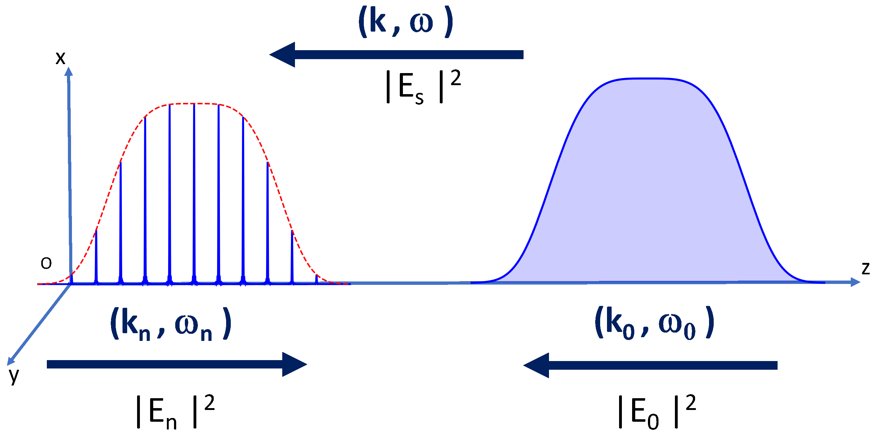
Here we assume a 2D geometry, as defined in Figure 1. In this geometry, two intense laser pulses, pulse 0 and pulse 1, counter-propagate along the z-direction. Photon-photon scattering will occur due to the nonlinear vacuum properties described by Equation (2). Notice that the high-harmonic pulse with frequencies can be described by a sequence of equidistant field spikes with amplitudes proportional to . This can be called superradiant scattering when the number of scattered photons is proportional to , where N is the number of intense spikes inside the pulse 1, with . This is a factor of N larger than the usual scattered intensity. Conditions for subradiance will also be found.
3. Incident Field
Let us first consider the primary field, associated with the two counter-propagating intense laser pulses. The incident (or pump) laser pulse can be described by the following electric field
where is the unit polarisation vector, the field amplitude, the phase, and the envelope function describing the pulse shape. We can use
for a Gaussian radial profile with beam waist , and a super-Gaussian axial profile with pulse duration . We assume propagation along z, as in Figure 1. On that figure, the intense pulse is arriving from the left, propagating in the negative z-direction. We use , and define the variable . Similarly, the counter-propagating high-harmonic pulse can be described by
with and . Here, the integer is the lowest harmonic inside the pulse. We also have
with , and , for . The high-harmonic pulse contains several high intensity spikes and propagates in the forward z-direction. In order to proceed, it is useful to consider nearly constant amplitudes for the different harmonics, . This simplifies the algebra and is also experimentally plausible. In reality, the amplitude of the harmonics vary slowly over a large spectral range, sometimes called the plateau, where a dependence of the form has been observed, for harmonic generation on a plasma mirror [22,33]. But this would change little to the present model, and will be ignored. This simplifying assumption allows us to write the summation over the harmonic spectrum as
with . Using the geometric series identity
we can write the field of the high-harmonic pulse (11) as
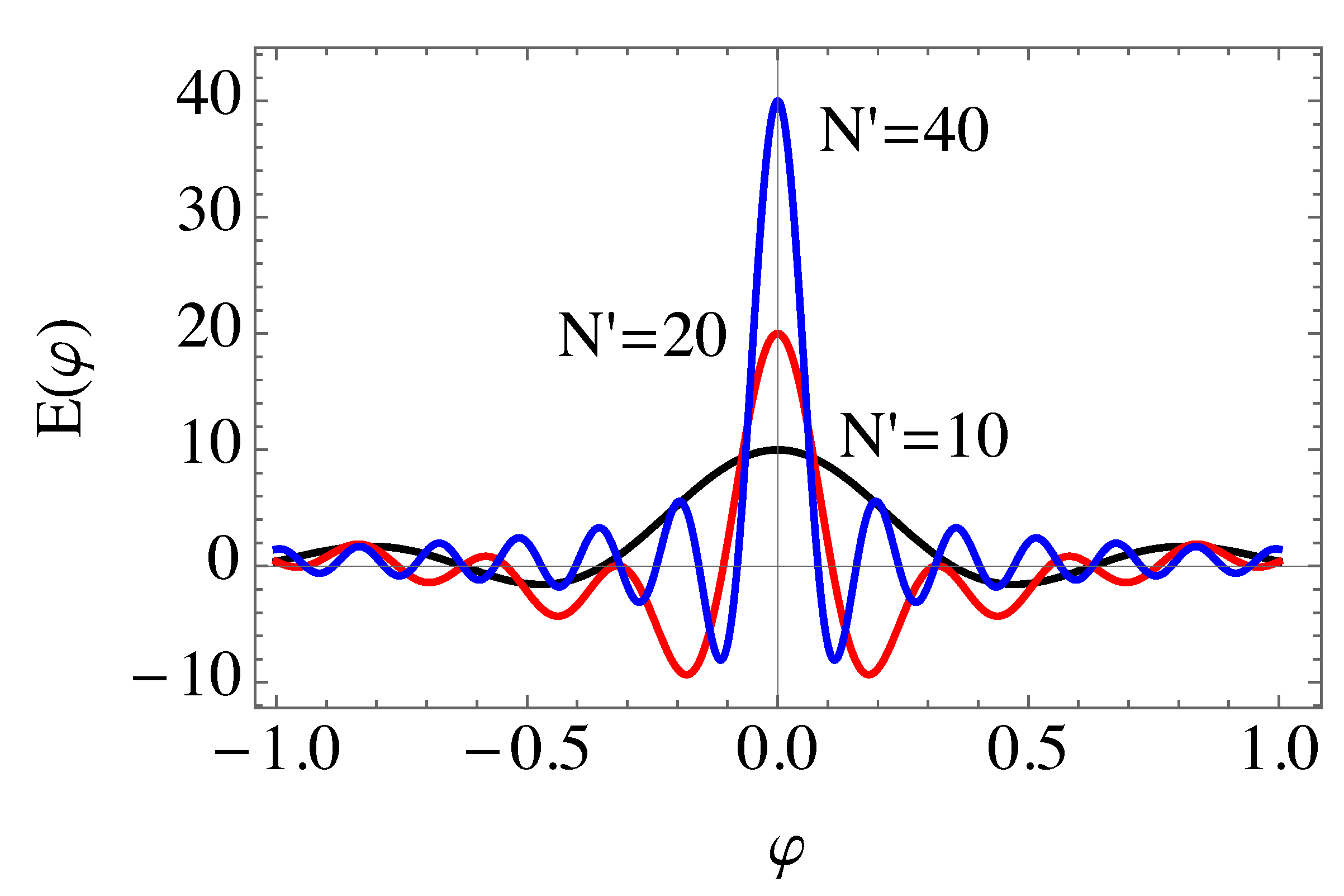
with . For a large number of harmonics , this represents a train of electric field spikes periodically located at , where is an integer. Noting that near these spikes, we have , we can rewrite this equation in a nearly equivalent form, as
where is the sine-cardinal function. See Figure 2 for an illustration.
Note that, in the limit of an infinite number of harmonics, we could also use a Dirac delta-function representation, due to the relation
In this limit, we could describe the field with the asymptotic expression
where the number of spikes is determined by . Neglecting the non-contributing terms associated with and , and using , we can define the quantity
with
where we have assumed that and to simplify. We have also neglected the temporal dependence of the envelope functions, which is approximately valid during the interaction time. On the other hand, the magnetic field will be polarised along , the same with . We can then calculate the field invariants and . Using Equation (4), we obtain
This would reduce, for a single harmonic , to expressions already found in the literature [32].
Notice that, if we take the limit defined by Equation (17), we arrive at the expression
where . A similar term could be written with replaced by , but is omitted for simplicity. We can now determine the frequency spectrum and amplitude of the secondary scattered fields , resulting from the interaction between the two laser pulses in vacuum. This field satisfies the propagation Equations (6) and (7) with source current (8). The fields appearing in the the nonlinear current are actually the total fields, but we can neglect the scattered fields and in the source terms, because they would only introduce negligible corrections to the vacuum dispersion. They can however be important if we want to describe other nonlinear vacuum effects, such as photon splitting or photon acceleration.
4. Secondary Field
Let us now study the scattered secondary fields in detail. In oder to calculate the source terms in Equation (7), we write
Neglecting higher order nonlinear corrections, this leads to the current
On the other hand, using and , Equation (21) allows us to write
with . A detailed analysis allows us to show that
On the other hand, it is also possible to show that [34]
where we usually have a laser beam waist much larger than the wavelength, . This means that, in the wave Equation (7) we can neglect the contribution from . If retained, this small contribution would lead to a scattered field in the perpendicular direction. We are then reduced to the following wave equation for the secondary scattered field
where S is defined in Equation (29).
5. Superradiant Scattering
Let us now consider the temporal Fourier spectrum of the scattered field, as defined by
Each Fourier component will therefore satisfy the wave equation
where
This allows us to write the equation for the scattered field, Equation (33), as
where the new amplitude for the source term is . We can also write this amplitude more explicitly as
where we have introduced the normalised QED vacuum factor R, as defined by Reference [34], and the normalised amplitude of the incident laser pulse , such that
For an estimate of the spectral intensity of the scattered radiation, we neglect the transverse dimensions, which are only relevant to define the slight deviations of the scattered radiation with respect to the z-axis. Contribution of transverse dimensions can easily be included, and will be briefly discussed later. Integration of Equation (37) for fields scattered in the backward direction, with , we get
Noting that the amplitude , as defined by Equation (38) but where the dependence on the radial direction was forgotten, is only nonzero in the interaction region, from minus to plus , we can then write, for the field at large distances ,
with
This integral is maximum for , which corresponds to forward scattering of the second harmonic of the incident field . This is experimentally relevant, because the frequency is not represented in the assumed incident fields, unless we exactly have .
In general, for a large interaction region such that , this integral is nearly zero , and no scattered field is expected. In the opposite case of a very short region, , the integral reduces to . Replacing this in Equation (41) we notice that this expression is dimensionally correct, as it should, because the quantities , and R are dimensionless, and has the same dimensions as the electric field . Furthermore, radiation will take place in a small range of values around . Equation (41) also shows that superradiant scattering occurs when the phases are all nearly equal. This occurs for , or , where n is an integer. This situation therefore corresponds to scattered frequencies equal to . In this case, the asymptotic value of the amplitude of the scattered field becomes
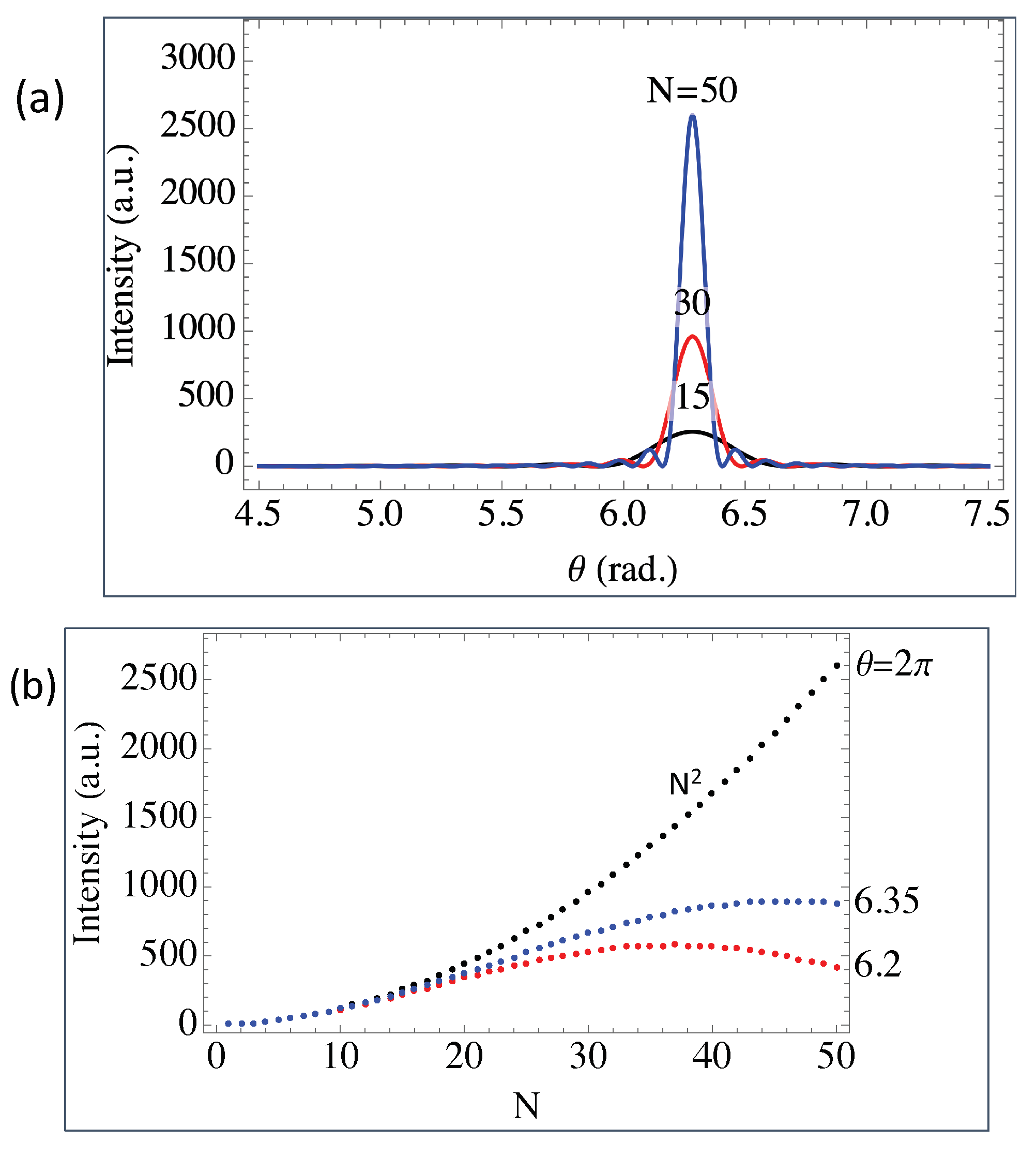
We therefore conclude that the scattered energy is proportional to the square of the number of spikes inside the high-harmonic pulse, , which is a characteristic signature of superradiance. This effect occurs when all the fields scattered by each spike are in phase, and constructively built the maximum possible value for the total field. The opposite case of subradiance could also occur, when and all the phase coherence is destroyed. In this extreme case, we will have a complete suppression of the vacuum nonlinearities. This is illustrated in Figure 3.
It is now appropriate to discuss the phase-matching conditions involved in superradiant scattering. For each harmonic , phase matching conditions stated in Section 2 would imply that , and . However, these two equalities cannot be satisfied simultaneously, because , except for the irrelevant case of . In our case, where n takes many different values, superradiant scattering is made of a superposition of several non-propagating fields, with phases determined by , and . Field superposition and phase-mixing then creates a single propagating field with , and , as shown in the above calculations. This means that the high-harmonic pulse acts as a kind of catalyser, building up an effective three-photon process which results from the superposition of forbidden four-photon mixing processes, such that two incident photons coalesce into a single superradiant photon. In this way, total energy and momentum conservation of quantum vacuum is automatically satisfied.
In the above description we have neglected the influence of the radial dimensions of the interaction pulses. This can easily be recovered, if we replace the amplitude appearing in Equation (42) by the transverse Fourier transform of the function , as defined in (38). This leads to the inclusion of a perpendicular vector potential in the scattered field , where . This will be negligible under plausible experimental conditions, when the transverse dimensions of the interaction region are much larger than the incident wavelength, .
Using Equation (43) and the plausible numbers of , , and , we can see that, for a sufficiently large number of spikes, , the ratio between scattered and high-harmonic field is of order . Noting that, for a near-infrared laser pulse we have , this field ratio will approach . It means that, for , we need incident photons to generate a single scattered photon. This gives typically one scattered photon per milliJoule of incident laser energy.
A more detailed analysis should take into account the finite spectral width of the interacting fields, which can be large for very short pulses. For Gaussian pulses, the amplitudes and should be replaced in Equations (9) and (11) by and , such that
and integration over should be added. The spectral width is limited by the pulse duration, as . This would lead to a small spectral width on the superradiant signal, not significantly changing the final result.
As a final comment, we note that the scattered field is independent of the number of harmonics . This counter-intuitive result is due to the fact that the amplitude of the electric field spikes is proportional to , but the interaction time associated with each spike decreases with , and the two effects exactly cancel. The same result is retrieved if, instead of delta-functions, we use sine-cardinal functions to describe the electric field spikes.
6. Conclusions
We have studied a new process associated with the nonlinear optical properties of the electromagnetic quantum vacuum, as predicted by QED in the weak field approximation. This corresponds to superradiant scattering of an intense laser pulse by a periodic array of intense electric field spikes which are associated with a counter-propagating pulse with a very large harmonic content. The spectral intensity of the scattered radiation was characterised, and conditions for the occurrence of superradiant scattering were defined.
We have shown that, under superradiant conditions, the number of scattered photons will be proportional to the square of the number of electric field spikes associated with the high-harmonic pulse, or . On the other hand, a subradiant suppression of QED effects, where vacuum nonlinearities seem to vanish, , could also take place. The number of spikes N can be very large, eventually of order . This would lead to an amplification of the number of photons emitted from vacuum of order . Given the recognised difficulty of detecting QED vacuum effects, which is due to the smallness of the vacuum factor R, this superradiant amplification could be significant in future experiments using ultra-intense lasers.
Funding
This research received no external funding.
Conflicts of Interest
The authors declare no conflict of interest.
References
- Danson, C.N.; Haefner, C.; Bromage, J.; Butcher, T.; Chanteloup, J.-C.F.; Chowdhury, E.A.; Galvanauskas, A.; Gizzi, L.A.; Hein, J.; Hillier, D.I.; et al. Petawatt and exawatt class lasers worldwide. High Power Laser Sci. Eng. 2019, 7, 54. [Google Scholar] [CrossRef]
- DiPiazza, A.; Muller, C.; Hatsagortsyan, K.Z.; Keitel, C.H. Extremely high-intensity laser interactions with fundamental quantum systems. Rev. Mod. Phys. 2012, 84, 20121177. [Google Scholar]
- Marklund, M.; Shukla, P.K. Nonlinear collective effects in photon-photon and photon-plasma interactions. Rev. Mod. Phys. 2006, 78, 591. [Google Scholar] [CrossRef] [Green Version]
- Ehlotzky, F.; Krajewska, K.; Zamiński, J.Z. Fundamental processes in quantum electrodymics in lasers fields of relativistic power. Rep. Prog. Phys. 2009, 72, 046401. [Google Scholar] [CrossRef]
- Zhang, P.; Bulanov, S.S.; Seipt, D.; Arefiev, A.V.; Thomas, A.G.R. Relativistic plasma physics in supercritical fields. Phys. Plasmas 2020, 27, 050601. [Google Scholar] [CrossRef]
- Schwinger, J. On gauge invariance and vacuum polarization. Phys. Rev. 1951, 82, 664. [Google Scholar] [CrossRef]
- Bulanov, S.S.; Narozhny, N.B.; Mur, V.D.; Popov, V.S. Electron-posiyron pair production for electromagnetic pulses. Sov. J. Exp. Theor. Phys. 2006, 102, 9. [Google Scholar] [CrossRef]
- Ruf, M.; Mocken, G.R.; Müller, C.; Hatsagortsyan, K.Z.; Keitel, C.H. Pair production in laser fields oscillating in space and time. Phys. Rev. Lett. 2009, 102, 080402. [Google Scholar] [CrossRef] [Green Version]
- Karplus, R.; Numan, M. The scattering of light by light. Phys. Rev. 1951, 83, 776. [Google Scholar] [CrossRef]
- Lundstrom, E.; Brodin, G.; Lundin, J.; Marklund, M.; Bingham, R.; Collier, J.; Mendonça, J.T.; Norreys, P. Using high-power lasers for detection of elastic photon-photon scattering. Phys. Rev. Lett. 2006, 96, 083602. [Google Scholar] [CrossRef] [Green Version]
- King, B.; Hu, H.; Shen, B. Three-pulse photon-photon scattering. Phys. Rev. A 2018, 98, 023817. [Google Scholar] [CrossRef] [Green Version]
- Bialynicka-Birula, Z.; Bialynicki-Birula, I. Nonlinear effects in Quantum Electrodynamics. Photon propagation and photon splitting in an external field. Phys. Rev. D 1970, 2, 2341. [Google Scholar] [CrossRef]
- Adler, S.L. Photon splitting and photon dispersion in a strong magnetic field. Ann. Phys. 1971, 67, 599–647. [Google Scholar] [CrossRef]
- Gies, H.; Karbstein, F.; Seegert, N. Quantum reflection of photons off spatio-temporal electromagnetic field inhomogeneities. New J. Phys. 2015, 17, 043060. [Google Scholar] [CrossRef] [Green Version]
- Mendonça, J.T.; Marklund, M.; Shukla, P.K.; Brodin, G. Photon acceleration in vacuum. Phys. Lett. A 2006, 359, 700–704. [Google Scholar] [CrossRef] [Green Version]
- Heisenberg, W.; Euler, H. Consequences of Dirac’s Theory of the Positron. Z. Phys. 1936, 98, 714–732. [Google Scholar] [CrossRef]
- Dunne, G.V. The Heisenberg-Euler effective action: 75 years on. Int. J. Mod. Phys. A 2012, 27, 1260004. [Google Scholar] [CrossRef] [Green Version]
- Klar, L. Detectable optical signatures of QED vacuum nonlinearities using high-intensity laser fields. Particles 2020, 3, 223–233. [Google Scholar] [CrossRef] [Green Version]
- Shibata, K. Intrinsic resonant enhancement of light by nonlinear vacuum. Eur. Phys. J. D 2020, 74, 215. [Google Scholar] [CrossRef]
- Paul, P.M.; Toma, E.S.; Berger, P.; Mullot, G.; Augé, F.; Balcou, P.; MUller, H.G.; Agostini, P. Observation of a train of attosecond pulses from high harmonic generation. Science 2001, 292, 1689–1692. [Google Scholar] [CrossRef]
- Vincenti, H.; Quéré, F. Attosecond lighthouses: How to use spatiotemporally coupled light fields to generate isolated attosecond pulses. Phys. Rev. Lett. 2012, 108, 113904. [Google Scholar] [CrossRef] [PubMed] [Green Version]
- Jahn, O.; Leshchenko, V.E.; Tzallas, P.; Kessel, A.; Krüger, M.; Münzer, A.; Trushin, S.A.; Tsakiris, G.D.; Kahaly, S.; Kormin, D.; et al. Towards intense isolated attosecond pulses from relativistic surface high harmonics. Optica 2019, 6, 280–287. [Google Scholar] [CrossRef] [Green Version]
- Dicke, R. Coherence in spontaneous radiation processes. Phys. Rev. 1954, 93, 99. [Google Scholar] [CrossRef] [Green Version]
- Rehler, N.E.; Eberly, J.H. Superradiance. Phys. Rev. A 1971, 3, 1735. [Google Scholar] [CrossRef]
- Gross, M.; Haroche, S. Superradiance: An essay on the theory of collective spontaneous emission. Phys. Rep. 1982, 93, 301–396. [Google Scholar] [CrossRef]
- Bonifacio, R.; McNeil, B.W.J.; Pierini, P. Superradiance in the high-gain free-electron laser. Phys. Rev. A 1989, 40, 4467. [Google Scholar] [CrossRef] [PubMed]
- Scully, M.O.; Svidzinsky, A.A. The super of superradiance. Science 2009, 325, 1510–1511. [Google Scholar] [CrossRef]
- Gover, A.; Ianconescu, R.; Friedman, A.; Emma, C.; Sudar, N.; Musumeci, P.; Pellegrini, C. Superradiant and stimulated-superradiant emission of bunched electron beams. Rev. Mod. Phys. 2019, 91, 035003. [Google Scholar] [CrossRef] [Green Version]
- Vieira, J.; Pardal, M.; Mendonça, J.T.; Fonseca, R.A. Generalized superradiance for producing broadband coherent radiation with transversely modulated arbitrarily diluted bunches. Nat. Phys. 2020. [Google Scholar] [CrossRef]
- Itzykson, C.; Zuber, J.-B. Quantum Field Theory; McGraw-Hill: New York, NY, USA, 1980. [Google Scholar]
- Dittrich, W.; Gies, H. Probing the Quantum Vacuum; Springer Tracts in Physics; Springer: Berlin/Heidelberg, Germany, 2000. [Google Scholar]
- Karbstein, F.; Shaisultanov, R. Stimulated photon emission from vacuum. Phys. Rev. D 2015, 91, 113002. [Google Scholar] [CrossRef] [Green Version]
- Baeva, T.; Gordienko, S.; Pukhov, A. Theory of high-order harmonic generation in relativistic laser interaction with overdense plasma. Phys. Rev. E 2006, 74, 046404. [Google Scholar] [CrossRef] [PubMed] [Green Version]
- Mendonça, J.T. Emission of twisted photons from quantum vacuum. EuroPhys. Lett. 2017, 120, 61001. [Google Scholar] [CrossRef]
Figure 1.
Geometry of the interaction: collision of an intense pulse with frequency with an intense high-harmonic pulse with frequencies . The intensity profiles of the two interacting pulses are represented, as well as the direction of their respective wavevectors. Nonlinear vacuum leads to the occurrence of a scattered signal with frequency .

Figure 2.
Electric field spikes due to a superposition of a large number of harmonics, as determined by Equation (16).
Figure 2.
Electric field spikes due to a superposition of a large number of harmonics, as determined by Equation (16).

Figure 3.
Scattered intensity as a function of the number of high harmonic field spikes N are represented, in arbitrary units, for different conditions of the inter-spike phase difference : (a) Intensity as a function of , for three different numbers of field spikes; (b) Intensity as a function of N for three different phase differences. Superradiance occurs for , and subradiance for .

Publisher’s Note: MDPI stays neutral with regard to jurisdictional claims in published maps and institutional affiliations. |
© 2021 by the author. Licensee MDPI, Basel, Switzerland. This article is an open access article distributed under the terms and conditions of the Creative Commons Attribution (CC BY) license (http://creativecommons.org/licenses/by/4.0/).
Share and Cite
MDPI and ACS Style
Mendonça, J.T. Superradiance in Quantum Vacuum. Quantum Rep. 2021, 3, 42-52. https://0-doi-org.brum.beds.ac.uk/10.3390/quantum3010003
AMA Style
Mendonça JT. Superradiance in Quantum Vacuum. Quantum Reports. 2021; 3(1):42-52. https://0-doi-org.brum.beds.ac.uk/10.3390/quantum3010003
Chicago/Turabian StyleMendonça, José Tito. 2021. "Superradiance in Quantum Vacuum" Quantum Reports 3, no. 1: 42-52. https://0-doi-org.brum.beds.ac.uk/10.3390/quantum3010003