Topological Quantum Computing and 3-Manifolds

Abstract

In this paper, we will present some ideas to use 3D topology for quantum computing. Topological quantum computing in the usual sense works with an encoding of information as knotted quantum states of topological phases of matter, thus being locked into topology to prevent decay. Today, the basic structure is a 2D system to realize anyons with braiding operations. From the topological point of view, we have to deal with surface topology. However, usual materials are 3D objects. Possible topologies for these objects can be more complex than surfaces. From the topological point of view, Thurston’s geometrization theorem gives the main description of 3-dimensional manifolds. Here, complements of knots do play a prominent role and are in principle the main parts to understand 3-manifold topology. For that purpose, we will construct a quantum system on the complements of a knot in the 3-sphere. The whole system depends strongly on the topology of this complement, which is determined by non-contractible, closed curves. Every curve gives a contribution to the quantum states by a phase (Berry phase). Therefore, the quantum states can be manipulated by using the knot group (fundamental group of the knot complement). The universality of these operations was already showed by M. Planat et al.

1. Introduction

Quantum computing exploits quantum-mechanical phenomena such as superposition and entanglement to perform operations on data, which in many cases, are infeasible to do efficiently on classical computers. The basis of this data is the qubit, which is the quantum analog of the classical bit. Many of the current implementations of qubits, such as trapped ions and superconductors, are highly susceptible to noise and decoherence because they encode information in the particles themselves. Topological quantum computing seeks to implement a more resilient qubit by utilizing non-Abelian forms of matter to store quantum information. In such a scheme, information is encoded not in the quasiparticles themselves, but in the manner in which they interact and are braided. In topological quantum computing, qubits are initialized as non-abelian anyons, which exist as their own antiparticles. Then, operations (what we may think of as quantum gates) are performed upon these qubits through braiding the worldlines of the anyons. Because of the non-Abelian nature of these particles, the manner in which they are exchanged matters (similar to non-commutativity). Another important property of these braids to note is that local perturbations and noise will not impact the state of the system unless these perturbations are large enough to create new braids. Finally, a measurement is taken by fusing the particles. Because anyons are their own antiparticles, the fusion will result in the annihilation of some of the particles, which can be used as a measurement. We refer to the book in [1] for an introduction of these ideas.

However, a limiting factor to use topological quantum computing is the usage of non-abelian anyons. The reason for this is the abelian fundamental group of a surface. Quantum operations are non-commutative operators leading to Heisenberg’s uncertainty relation, for instance. Non-abelian groups are at the root of these operators. Therefore, if we use non-abelian fundamental groups instead of abelian groups, then (maybe) we do not need non-abelian states to realize quantum computing. In this paper, we discuss the usage of (non-abelian) fundamental groups of 3-manifolds for topological quantum computing. At first, quantum gates are elements of the fundamental group represented as $SU\left(2\right)$ matrices. The set of possible operations depends strongly on the knot, i.e., the topology. The fundamental group is a topological invariant, thus making this representation of quantum gates part of topological quantum computing. In principle, we have two topological ingredients: the knot and the fundamental group of the knot complement. The main problem now is how these two ingredients can be realized in a quantum system. In contrast to topological quantum computing with anyons, we cannot directly use 3-manifolds (as submanifolds) like surfaces in the fractional Quantum Hall effect. Surfaces (or 2-manifolds) embed into a 3-dimensional space like ${\mathbb{R}}^3$ but 3-manifolds require a 5-dimensional space like ${\mathbb{R}}^5$ as an embedding space. Therefore, we cannot directly use 3-manifolds. However, as we will argue in the next section, there is a group-theoretical substitute for a 3-manifolds, the fundamental group of a knot complement also known as knot group. Then, we will discuss the knot group of the simplest knot, the trefoil. The knot group is the braid group of three strands used for anyons too. The 1-qubit gates are given by the representation of the knot group into the group $SU\left(2\right)$. Here, one can get all 1-qubit operations by this method. For an application of these fundamental group representations to topological quantum computing, we need a realization of the fundamental group in a quantum systems. Here, we will refer to the one-to-one connection between the holonomy of a flat $SU\left(2\right)$ connection (i.e., vanishing curvature) and the representation of fundamental group into $SU\left(2\right)$. Here, we will use the Berry phase but the corresponding Berry connection admits a non-vanishing curvature. However, we will show that one can rearrange the Berry connection for two-level systems to get a flat $SU\left(2\right)$ connection. Then, the holonomy along this connection only depends on the topology of the knot complement so that the manipulation of states are topologically induced. All $SU\left(2\right)$-representation of the knot group form the so-called character variety which contains important information about the knot complement (see in [2] for instance). However, the non-triviality of the character variety can be interpreted that knot groups give the 1-qubit operations. In Section 6, we will discuss the 2-qubit operations by linking two knots. Here, every link component carries a representation into $SU\left(2\right)$. The relation in the fundamental group induces the interaction term. The interaction terms are known from the Ising model. Therefore, finally we get a complete set of operations to realize any quantum circuit: a 1-qubit operation by the knot group of the trefoil knot and a 2-qubit operation by the complement of the link (Hopf link for instance). For the universality of these operations we refer to the work of M. Planat et al. [3,4], which was the main inspiration of this work. This paper followed the idea to use knots directly for quantum computing. In the focus is the knot complement which is the space outside of a knot. Then, the knot is one system and the space outside is a second system. Currently, the author is working on the concrete realization of this idea. In this paper, I will present the idea in an abstract manner to clarify whether knot complements are suitable for quantum computing from informational point of view.

The usage of knots in physics but also biology is not new. One of the pioneers is Louis H. Kauffman, and we refer to his book [5] for many relations between knot theory and natural science. Furthermore, note his ideas about topological information [6] (see also in [7,8]). Knots are also important models in quantum gravity, see, for instance, in [9], and in particle physics [10,11,12].

2. Some Preliminaries and Motivation: 3-Manifolds and Knot Complements

The central concept for the following paper is the concept of a smooth manifold. To present this work as self-contained as possible, we will discuss some results in the theory of 2- and 3-dimensional manifolds which is the main motivation for this paper. At first we will give the formal definition of a manifold:

• Let M be a Hausdorff topological space covered by a (countable) family of open sets, $\mathcal{U}$, together with homeomorphisms, ${\varphi }_U:U\in \mathcal{U}\to U_R,$ where $U_R$ is an open set of ${\mathbb{R}}^n.$ This defines M as a topological manifold. For smoothness we require that, where defined, ${\varphi }_U·{\varphi }_V^{-1}$ is smooth in ${\mathbb{R}}^n,$ in the standard multivariable calculus sense. The family $\mathcal{A}=\{\mathcal{U},{\varphi }_U\}$ is called an atlas or a differentiable structure. Obviously, $\mathcal{A}$ is not unique. Two atlases are said to be compatible if their union is also an atlas. From this comes the notion of a maximal atlas. Finally, the pair $(M,\mathcal{A})$, with $\mathcal{A}$ maximal, defines a smooth manifold of dimension n.
• An important extension of this construction yields the notion of smooth manifold with boundary, M, defined as above, but with the atlas such that the range of the coordinate maps, $U_R,$ may be open in the half space, ${\mathbb{R}}_{+}^n$, that is, the subspace of ${\mathbb{R}}^n$ for which one of the coordinates is non-positive, say $x^n\le 0.$ As a subspace of ${\mathbb{R}}^n,{\mathbb{R}}_{+}^n$ has a topologically defined boundary, namely, the set of points for which $x^n=0.$ Use this to define the (smooth) boundary of $M,\partial M,$ as the inverse image of these coordinate boundary points.

In the following, we will concentrate on the special theory of 2- and 3-manifolds (i.e., manifolds of dimension 2, surfaces, or 3). The classification of 2-manifolds has been known since the 19th century. In contrast, the corresponding theory for 3-manifolds based on ideas of Thurston around 1980 but was completed 10 years ago. In both cases—2- and 3-manifolds—the manifold is decomposed by the operation $M\#N$, the connected sum.

Let $M,N$ be two n-manifolds with boundaries $\partial M,\partial N$. The connected sum $M\#N$ is the procedure of cutting out a disk $D^n$ from the interior $int\left(M\right)\backslash D^n$ and $int\left(N\right)\backslash D^n$ with the boundaries $S^{n-1}\bigsqcup \partial M$ and $S^{n-1}\bigsqcup \partial N$, respectively, and gluing them together along the common boundary component $S^{n-1}$.

For 2-manifolds, the basic elements are the 2-sphere $S^2$, the torus $T^2$ or the Klein bottle $\mathbb{R}{P}^2$. Then, one gets for the classification of 2-manifolds:

• Every compact, closed, oriented 2-manifold is homeomorphic to either $S^2$ or the connected sum

  $$\underset{g}{\underbrace{T^2\#T^2\#\dots \#T^2}}$$

  of $T^2$ for a fixed genus g. Every compact, closed, non-oriented 2-manifold is homeomorphic to the connected sum

  $$\underset{g}{\underbrace{\mathbb{R}{P}^2\#\mathbb{R}{P}^2\#\dots \#\mathbb{R}{P}^2}}$$

  of $\mathbb{R}{P}^2$ for a fixed genus g.
• Every compact 2-manifold with boundary can be obtained from one of these cases by cutting out the specific number of disks $D^2$ from one of the connected sums.

A connected 3-manifold N is prime if it cannot be obtained as a connected sum of two manifolds $N_1\#N_2$ neither of which is the 3-sphere $S^3$ (or, equivalently, neither of which is the homeomorphic to N). Examples are the 3-torus $T^3$ and $S^1\times S^2$, but also the Poincare sphere. According to the work in [13], any compact, oriented 3-manifold is the connected sum of an unique (up to homeomorphism) collection of prime 3-manifolds (prime decomposition). A subset of prime manifolds are the irreducible 3-manifolds. A connected 3-manifold is irreducible if every differentiable submanifold S homeomorphic to a sphere $S^2$ bounds a subset D (i.e., $\partial D=S$) which is homeomorphic to the closed ball $D^3$. The only prime but reducible 3-manifold is $S^1\times S^2$.

For the geometric properties (to meet Thurston’s geometrization theorem) we need a finer decomposition induced by incompressible tori. A properly embedded connected surface $S\subset N$ is called 2-sided (The “sides” of S then correspond to the components of the complement of S in a tubular neighborhood $S\times [0,1]\subset N$.) if its normal bundle is trivial, and 1-sided if its normal bundle is nontrivial. A 2-sided connected surface S other than $S^2$ or $D^2$ is called incompressible if for each disk $D\subset N$ with $D\cap S=\partial D$ there is a disk $D^{\prime }\subset S$ with $\partial D^{\prime }=\partial D$. The boundary of a 3-manifold is an incompressible surface. Most importantly, the 3-sphere $S^3$, $S^2\times S^1$ and the 3-manifolds $S^3/\Gamma$ with $\Gamma \subset SO\left(4\right)$ a finite subgroup do not contain incompressible surfaces. The class of 3-manifolds $S^3/\Gamma$ (the spherical 3-manifolds) include cases like the Poincare sphere ($\Gamma =I^{*}$ the binary icosaeder group) or lens spaces ($\Gamma ={\mathbb{Z}}_p$ the cyclic group). Let $K_i$ be irreducible 3-manifolds containing incompressible surfaces then we can N split into pieces (along embedded $S^2$)

$$N=K_1\#\cdots \#K_{n_1}{\#}_{n_2}{S}^1\times S^2{\#}_{n_3}{S}^3/\Gamma ,$$

(1)

where ${\#}_n$ denotes the n-fold connected sum and $\Gamma \subset SO\left(4\right)$ is a finite subgroup. The decomposition of N is unique up to the order of the factors. The irreducible 3-manifolds $K_1,\dots ,K_{n_1}$ are able to contain incompressible tori and one can split $K_i$ along the tori into simpler pieces $K=H{\cup }_{T^2}G$ [14] (called the JSJ decomposition). The two classes G and H are the graph manifold G and hyperbolic 3-manifold H.

In 1982, W.P. Thurston presented a program intended to classify smooth 3-manifolds and solve the Poincare conjecture by investigating the possible geometries on such 3-manifolds. For a survey of this topic see in [15]. The key ingredient of this classification ansatz is the concept of a model geometry. Again, in this section, all manifolds are assumed to be smooth.

A model geometry $(G,X)$ consists of a simply connected manifold X together with a Lie group G of diffeomorphisms acting transitively on X fulfilling certain set of conditions. One of these is that there is a G-invariant Riemannian metric. For example, reducing the dimension, we can consider 2-dimensional model geometries of a 2-manifold X. From Riemannian geometry, we know that any G-invariant Riemannian metric on X has constant Gaussian curvature (recall that G must be transitive). A constant scaling of the metric allows us to normalize the curvature to be 0, 1, or $-1$ corresponding to the Euclidean (${\mathbb{E}}^2$), spherical ($S^2$) and hyperbolic (${\mathbb{H}}^2$) space, respectively. Thus, there are precisely three two-dimensional model geometries: spherical, Euclidean, and hyperbolic.

It is a surprising fact that there are also a finite number of three-dimensional model geometries. It turns out that there are eight geometries: spherical, Euclidean, hyperbolic, mixed spherical-Euclidian, mixed hyperbolic-Euclidian, and three exceptional cases. A geometric structure on a more general manifold M (not necessarily simply connected) is defined by a model geometry $(G,X)$ where X is the universal covering space to M, i.e., $M=X/{\pi }_1\left(M\right)$. This is equivalent to a representation ${\pi }_1\left(M\right)\to G$ of the fundamental group into G. Of course a geometric structure on a 3-manifold may not be unique but Thurston explored decompositions into pieces each of which admit a unique geometric structure. This decomposition proceeds by splitting M into essentially unique pieces using embedded 2-spheres and 2-tori in such a way that a model geometry can be defined on each piece. Thus,

• Thurston’s Geometrization conjecture can be stated:
  The interior of every compact 3-manifold has a canonical decomposition into pieces (described above), which have one of the eight geometric structures.
  In short, every 3-manifold can be uniquely decomposed (long 2-spheres) into prime manifolds where some of these prime manifolds can be further split (along 2-tori) into graph G and hyperbolic manifolds H. Then, $G,H$ have a disjoint union of 2-tori as boundary; but how can we construct these manifolds having a geometric structure? A knot in mathematics is the embedding of a circle into the 3-sphere $S^3$ (or in ${\mathbb{R}}^3$), i.e., a closed knotted curve. Let K be a prime knot (a knot not decomposable by a sum of two knots). With $K\times D^2$ we denote a thicken knot, i.e., a closed knotted solid torus. The knot complement $C\left(K\right)=S^3\backslash \left(K\times D^2\right)$ is a 3-manifold with boundary $\partial C\left(K\right)=T^2$. It was shown that prime knots are divided into two classes: hyperbolic knots ($C\left(K\right)$ admits a hyperbolic structure) and non-hyperbolic knots ($C\left(K\right)$ admits one of the other seven geometric structures). An embedding of disjoints circles into $S^3$ is called a link $L.$ Then, $C\left(L\right)$ is the link complement. Here, the situation is more complicated: $C\left(L\right)$ can admit a geometric structure or it can be decomposed into pieces with a geometric structure. $C\left(L\right),C\left(K\right)$ are one of the main models for G or H for suitable knots and links. If we speak about 3-manifolds then we have to consider $C\left(K\right)$ as one of the basic pieces. Furthermore, there is the Gordon–Luecke theorem: if two knot complements are homeomorphic, then the knots are equivalent (see in [16] for the statement of the exact theorem). Interestingly, knot complements of prime knots are determined by its fundamental group. For the fundamental group, one considers closed curves which are not contractible. Furthermore, two curves are equivalent if one can deform them into each other (homotopy relation). The concatenation of curves can be made into a group operation up to deformation equivalence (i.e., homotopy). Formally, it is the set of homotopy classes $[S^1,X]$ of maps $S^1\to X$ (the closed curves) into a space X up to homopy, denoted by ${\pi }_1\left(X\right)$. The fundamental group ${\pi }_1\left(C\left(K\right)\right)$ of the knot complement is also known as knot group. Here, we refer to the books in [5,17,18] for a good introduction into this theory. The main idea of this paper is the usage of the knot group as substitute for a 3-manifold and try to use this group for quantum computing.

3. Knot Complement of the Trefoil Knot and the Braid Group ${\mathit{B}}_{\mathbf{3}}$

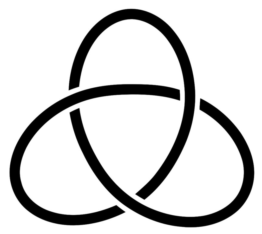
Any knot can be represented by a projection on the plane with no multiple points which are more than double. As an example let us consider the simplest knot, the trefoil knot $3_1$ (knot with three crossings).

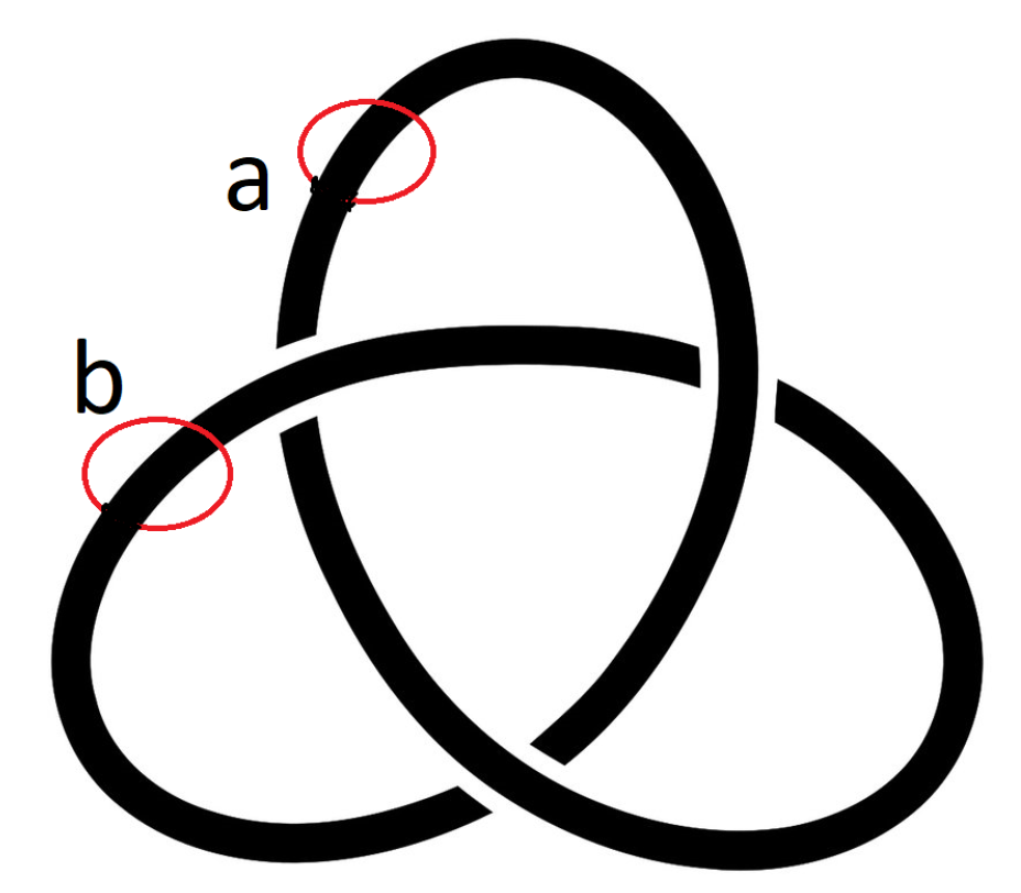
The plane projection of the trefoil is shown in Figure 1. This projection can be divided into three arcs, around each arc we have a closed curve as generator of ${\pi }_1\left(C\left(3_1\right)\right)$ denoted by $a,b,c$ (see also Figure 2 for the definition of the generators $a,b$). Now each crossing gives a relation between the corresponding generators: $c=a^{-1}ba,b=c^{-1}ac,a=b^{-1}cb$, i.e., we get the knot group

$${\pi }_1\left(C\left(3_1\right)\right)=\langle a,b,c|c=a^{-1}ba,b=c^{-1}ac,a=b^{-1}cb\rangle$$

Then, we substitute the expression $c=a^{-1}ba$ into the other relations to get a representation of the knot with two generators and one relation. From relation $a=b^{-1}cb$ we will obtain $a=b^{-1}\left(a^{-1}ba\right)b$ or $bab=aba$ and the other relation $b=c^{-1}ac$ gives nothing new. Finally, we will get the well-known result

$${\pi }_1\left(C\left(3_1\right)\right)=\langle a,b|bab=aba\rangle$$

However, this group is also well known; it is the braid group $B_3$ of three strands. In general, the braid group $B_n$ is generated by $\left\{1,{\sigma }_1,\dots ,{\sigma }_{n-1}\right\}$ subject to the relations (see in [18])

$${\sigma }_i{\sigma }_{i+1}{\sigma }_i={\sigma }_{i+1}{\sigma }_i{\sigma }_{i+1}{\sigma }_i{\sigma }_j={\sigma }_j{\sigma }_i|i-j|>1$$

For $B_3$ we have two generators ${\sigma }_1,{\sigma }_2$ with one relation ${\sigma }_1{\sigma }_2{\sigma }_1={\sigma }_2{\sigma }_1{\sigma }_2$ agreeing with ${\pi }_1\left(C\left(3_1\right)\right)$. The braid group $B_3$ has connections to different areas. Notable is the relation to the modular group $SL(2,\mathbb{Z})$ (the group of integer $2\times 2$ matrices with unit determinant) generated by

$$S=\left(\begin{array}{cc}0& 1\\ -1& 0\end{array}\right)U=\left(\begin{array}{cc}1& 1\\ -1& 0\end{array}\right)$$

It is well-known that $B_3$ maps surjectively onto $SL(2,\mathbb{Z})$ via the map

$${\sigma }_1\mapsto \left(\begin{array}{cc}1& 1\\ 0& 1\end{array}\right){\sigma }_2\mapsto \left(\begin{array}{cc}1& 0\\ -1& 1\end{array}\right)$$

However, then ${\sigma }_1{\sigma }_2{\sigma }_1={\sigma }_2{\sigma }_1{\sigma }_2$ maps to S and ${\sigma }_1{\sigma }_2$ maps to U. It is interesting to note that ${\left({\sigma }_1{\sigma }_2\right)}^3$ is in the center Z of $B_3$ (i.e., this elements commutes with all other elements) and $B_3/Z=SL(2,\mathbb{Z})/\left\{\pm 1\right\}$, or $B_3$ is the central extension of $PSL(2,\mathbb{Z})=SL(2,\mathbb{Z})/\left\{\pm 1\right\}$ (the $(2,3,\infty )$ triangle group) by the integers $\mathbb{Z}$ (see [12] for an application of this relation in physics).

4. Using the Trefoil Knot Complement for Quantum Computing

In this section, we will get in touch with quantum computing. The main idea is the interpretation of the braid group $B_3$ as operations (gates) on qubits. From the mathematical point of view, we have to consider the representation of $B_3$ into $SU\left(2\right)$, i.e., a homomorphism

$$\varphi :B_3\to SU\left(2\right)$$

mapping sequences of generators (called words) into matrices as elements of $SU\left(2\right)$. For completeness we will study some representations. Here, we follow the work in [19] to illustrate the general theory. At first, we note that a matrix in $SU\left(2\right)$ has the form

$$M=\left(\begin{array}{cc}z& w\\ -\overline{w}& \overline{z}\end{array}\right){\left|z\right|}^2+{\left|w\right|}^2=1$$

where z and w are complex numbers. Now we choose a well-known basis of $SU\left(2\right)$:

$$\mathbf{1}=\left(\begin{array}{cc}1& 0\\ 0& 1\end{array}\right)\mathit{i}=\left(\begin{array}{cc}i& 0\\ 0& -i\end{array}\right)\mathit{j}=\left(\begin{array}{cc}0& 1\\ -1& 0\end{array}\right)\mathit{k}=\left(\begin{array}{cc}0& i\\ i& 0\end{array}\right)$$

(2)

so that

$$M=a\mathbf{1}+b\mathit{i}+c\mathit{j}+d\mathit{k}$$

with $a^2+b^2+c^2+d^2=1$ (and $z=a+bi,w=c+di$). The algebra of $\mathbf{1},\mathit{i},\mathit{j},\mathit{k}$ are known as quaternions (with relations $ij=k$, $I^2=j^2=k^2=-1$). In the following, we will switch between the usual basis $1,i,j,k$ of the quaternions and the matrix representation with basis $\mathbf{1},\mathit{i},\mathit{j},\mathit{k}$, see (2). Then, the unit quaternions (of length 1) can be identified with the elements of $SU\left(2\right)$. Pure quaternions are defined by all expressions $b\mathit{i}+c\mathit{j}+d\mathit{k}$ (i.e., $a=0$). Now, the homomorphism $\varphi$ above is the mapping

$$g=\varphi \left({\sigma }_1\right),h=\varphi \left({\sigma }_2\right)$$

so that $ghg=hgh$. Let $u,v$ be pure quaternions of length 1 (unit, pure quaternions). Now, for $g=a+bu$ and $h=c+dv$ we have to choose

$$g=a+bu,h=a+bv,bu·bv=a^2-\frac{1}{2}$$

(see in [19] for the proof) for the image of the homomorphism $\varphi$ then the relation of the $B_3$ is fulfilled, or we have a representation of $B_3$ into $SU\left(2\right)$.

For more practical scenarios this general representation is the following construction. Let us choose

$$g=e^{i\theta }=a+b\mathrm{i}$$

where $a=cos\left(\theta \right)$ and $b=sin\left(\theta \right).$ Let

$$h=a+b\left[(c^2-s^2)i+2cs·k\right]$$

where $c^2+s^2=1$ and $c^2-s^2=\frac{a^2-b^2}{2b^2}$. Then we are able to rewrite $g,h$ as matrices $G,H$. In principle, the matrices $G,H$ can be obtained from the expressions above by a switch of the basis, i.e.,

$$G=exp\left(\theta \mathit{i}\right)H=a\mathbf{1}+b\left[(c^2-s^2)\mathit{i}+2cs\mathit{k}\right]$$

Here, we choose $H=FG{F}^{+}$ and

$$G=\left(\begin{array}{cc}{e}^{i\theta }& 0\\ 0& e^{-i\theta }\end{array}\right)F=\left(\begin{array}{cc}ic& is\\ is& -ic\end{array}\right)$$

Among this class of representations, there is the simplest example

$$g=e^{7\pi i/10},f=i\tau +k\sqrt{\tau },h=fg{f}^{-1}$$

where ${\tau }^2+\tau =1$. Then, $g,h$ satisfy $ghg=hgh$ the relation of $B_3$. This representation is known as the Fibonacci representation of $B_3$ to $SU\left(2\right)$. The Fibonacci representation is dense in $SU\left(2\right)$, see [1]. This representation is generated by the 20th root of unity. Other dense representations are given by $4r$th roots of unity via recoupling theory, see Sections 1.3 and 1.4 in [1].

5. Knot Group Representations via Berry Phases

In the previous section we discussed, the representations of the knot group into $SU\left(2\right)$ to realize the 1-qubit operations. Central point in this paper is the representation

$$\varphi :{\pi }_1\left(C\left(K\right)\right)\to SU\left(2\right)$$

of the knot group. The fundamental group is a topological invariant and we have to realize this group in a quantum system. In this section, we will realize these 1-qubit gates, the 2-qubit gate will be described in the next section. Here, we will discuss the direct realization of the knot group, i.e., the fundamental group of the knot complement. We will not discuss the abstract representation of the group ${\pi }_1\left(C\left(K\right)\right)$ by quantum gates which is also possible. For that purpose we have to define the fundamental group more carefully. Let X be a topological space or a manifold. A map $\gamma :[0,1]\to X$ with $\gamma \left(0\right)=\gamma \left(1\right)$ is a closed curve. Two curves ${\gamma }_1,{\gamma }_2$ are homotopic ${\gamma }_1\simeq {\gamma }_2$ if there is a one-parameter family of continuous maps which deform ${\gamma }_1$ to ${\gamma }_2$. The concatenation ${\gamma }_1\#{\gamma }_2$ of curves (up to homotopy) is the group operation making the set of homotopy classes of closed curves to a group, the fundamental group ${\pi }_1\left(X\right)$. Now, we will discuss the representation of the fundamental group by the holonomy along a closed curve, i.e., by an integral of a gauge connection or potential along a closed curve. As shown by Milnor [20], there is one-to-one relation between a homomorphism ${\pi }_1\left(X\right)\to G$ into the Lie group G and the integral

$${\displaystyle \underset{\gamma }{\oint }A}withdA+A\wedge A=0$$

of a flat G-connection A, i.e., this integral depends only on the homotopy class of the closed curve $\gamma$. In our case, we will interpret the representation

$$\varphi :{\pi }_1\left(C\left(K\right)\right)\to SU\left(2\right)$$

up to conjugation as a flat connection of a $SU\left(2\right)$ principal bundle over the knot complement $C\left(K\right)$. Let P be a $SU\left(2\right)$ principal fiber bundle over $C\left(K\right)$ with connection A locally represented by a 1-form with values in the adjoint representation of the Lie algebra $\mathfrak{su}\left(2\right)$, i.e., $A\in {\Lambda }^1\left(C\left(K\right)\right)\otimes ad\left(\mathfrak{su}\left(2\right)\right)$. The connection is flat if the curvature

$$F=dA+A\wedge A=0$$

vanishes. In this case (see Milnor [20]) the integral

$${\displaystyle \underset{\gamma }{\oint }A}$$

along a closed curve $\gamma :S^1\to C\left(K\right)$ depends only on the homotopy class $\left[\gamma \right]\in {\pi }_1\left(C\left(K\right)\right)$ and the exponential

$${\pi }_1\left(C\left(K\right)\right)\ni \gamma \to \varphi \left(\gamma \right)=\mathcal{P}exp\left({\displaystyle \underset{\gamma }{\oint }A}\right)\in SU\left(2\right)$$

for varying closed curves ($\mathcal{P}$ path ordering operator) gives a representation ${\pi }_1\left(C\left(K\right)\right)\to SU\left(2\right)$. However, which quantum system realized this representation? Let us consider the Hamiltonian

$$H=H_0+h$$

with a non-adiabatic and adiabatic part. The whole Hamiltonian has to fulfill the usual Schrödinger equation

$$iħ\frac{\partial }{\partial t}|\psi \rangle =H|\psi \rangle$$

and we have to demand that each eigenstate $|k_n\rangle$ of the Hamiltonian h with discrete spectrum

$$h|k_n\rangle =E_n|k_n\rangle$$

develops independently in time. Then, we have the decomposition

$$|\psi \rangle =\sum _n{a}_n|k_n\rangle$$

leading to the solution

$$a_n=exp\left(-\frac{i}{ħ}\int E_n\left(\tau \right)d\tau \right)exp\left(\int \langle k_n\left|\frac{\partial }{\partial \tau }\right|k_n\rangle d\tau \right)$$

where the second expression is known as geometric phase or Berry phase. Usually the states are parameterized by some manifold M with coordinates $x=x\left(t\right)$ and we consider a cyclic evolution $x\left(0\right)=x\left(T\right)$, i.e., closed curves in M. Then, the Berry phase is given by

$${\theta }_{top}={\displaystyle \underset{\gamma }{\oint }}\langle k_n\left|d\right|k_n\rangle$$

and the expression $A_{Berry}=\langle k_n\left|d\right|k_n\rangle$ as Berry connection. This solution is well known and for completeness we described it here again. At first, the Berry connection is the connection of $U\left(1\right)$ principal bundle. Second, the curvature $\Omega =d{A}_{Berry}$ is non-zero. Therefore, at the first view we cannot use this connection to represent the knot group. We need a connection with values in $SU\left(2\right)$ to get a representation for $\varphi$ via $exp\left({\theta }_{top}\right)$. Our idea is now to rearrange the components of the Berry connection (including the off-diagonal terms) to produce a $SU\left(2\right)$ connection. For that purpose, we will restrict the system to a 2-level system, $|k_0\rangle ,|k_1\rangle$. Then, we remark that the Lie algebra $\mathfrak{su}\left(2\right)$ is generated by the three Pauli matrices ${\sigma }_x,{\sigma }_y,{\sigma }_z$ so that every element is given by a linear combination $a·{\sigma }_x+b·{\sigma }_y+c·{\sigma }_z$. Now we arrange the possible connection components ${\omega }_{nm}=\langle k_n\left|d\right|k_m\rangle$ into one matrix

$$\omega =\left(\begin{array}{cc}\langle k_0\left|d\right|k_0\rangle & \langle k_0\left|d\right|k_1\rangle \\ \langle k_1\left|d\right|k_0\rangle & \langle k_1\left|d\right|k_1\rangle \end{array}\right)$$

with the decomposition

$$\omega =\langle k_0\left|d\right|k_0\rangle \frac{\mathbf{1}+{\sigma }_z}{2}+\langle k_1\left|d\right|k_1\rangle \frac{\mathbf{1}-{\sigma }_z}{2}+\Re (\langle k_0\left|d\right|k_1\rangle ){\sigma }_x+\Im \langle k_0\left|d\right|k_1\rangle {\sigma }_y$$

By using the normalization $\langle k_n|k_m\rangle ={\delta }_{nm}$ one gets

$$0=d\left(\langle k_n|k_m\rangle \right)={\omega }_{nm}^{*}+{\omega }_{nm}$$

and

$$d{\omega }_{nm}=\sum _k{\omega }_{nk}^{*}\wedge {\omega }_{km}=-\sum _k{\omega }_{nk}\wedge {\omega }_{km}$$

so that we obtain for the curvature $\Omega$

$$\Omega =d\omega +\omega \wedge \omega =0$$

Obviously $\omega$ is a connection of a flat $SU\left(2\right)$ bundle and the integral

$${\displaystyle \underset{\gamma }{\oint }}\omega$$

depends only on the homotopy class of the closed curve $\gamma$, as we want. The off-diagonal terms like $\langle k_0\left|d\right|k_1\rangle$ of the connection $\omega$ can be calculated with respect to the expectation values of $dh$. Together with the eigenvalues $E_0,E_1$ of h for $|k_0\rangle ,|k_1\rangle$, respectively, we obtain, for instance,

$$\langle k_0\left|d\right|k_1\rangle =\frac{\langle k_0\left|dh\right|k_1\rangle }{E_0-E_1}$$

Then, the exponential of this integral gives a representation $\varphi$ of the fundamental group into $SU\left(2\right).$ Now we go back to the trefoil knot complement $C\left(3_1\right)$ with fundamental group ${\pi }_1\left(C\left(3_1\right)\right)=B_3$. Then, the Berry phases along the two generators $a,b$ (i.e., two closed curves) of the fundamental group ${\pi }_1\left(C\left(3_1\right)\right)=B_3$ generate the 1-Qubit operations. Via the Berry phases, these operations act on the quantum system to influence its state. Keeping this idea in mind, we have the following scheme: consider a qubit on the trefoil knot and consider the two generators $a,b$ of the knot group (see Figure 2).

If we do manipulations along these two closed curves we are able to influence the qubit by using the Berry phase. Here, we refer to the work [21] for ideas to use the Berry phase for quantum computing.

6. Linking and 2-Qubit Operations

In the previous section, we described the appearance of the braid group $B_3$ as fundamental group of the trefoil knot complement. Above we described the situation that the knot complement of the trefoil knot determines the operations or quantum gates. In this case, the quantum gates are braiding operations (used for anyons) for three-strand braids. Unfortunately, the $SU\left(2\right)$—representations of the braid group $B_3$ are only 1-qubit gates but one needs at least a 2-qubit gate like CNOT to represent any quantum circuit. It is known that for 2-qubit operations, one needs elements of the braid group $B_6$. Is there other knot complements having braid groups as fundamental groups? Unfortunately, the answer is no. Here, is the line of arguments: every knot complement is determined by the fundamental group (aspherical space), then the cohomology of knot complements is determined by the first two groups (0th and 1th), all other groups are given by duality. But the braid groups $B_n$ for $n>3$ have non-trivial cohomology groups in degree 3 or higher which is impossible for knot complements.

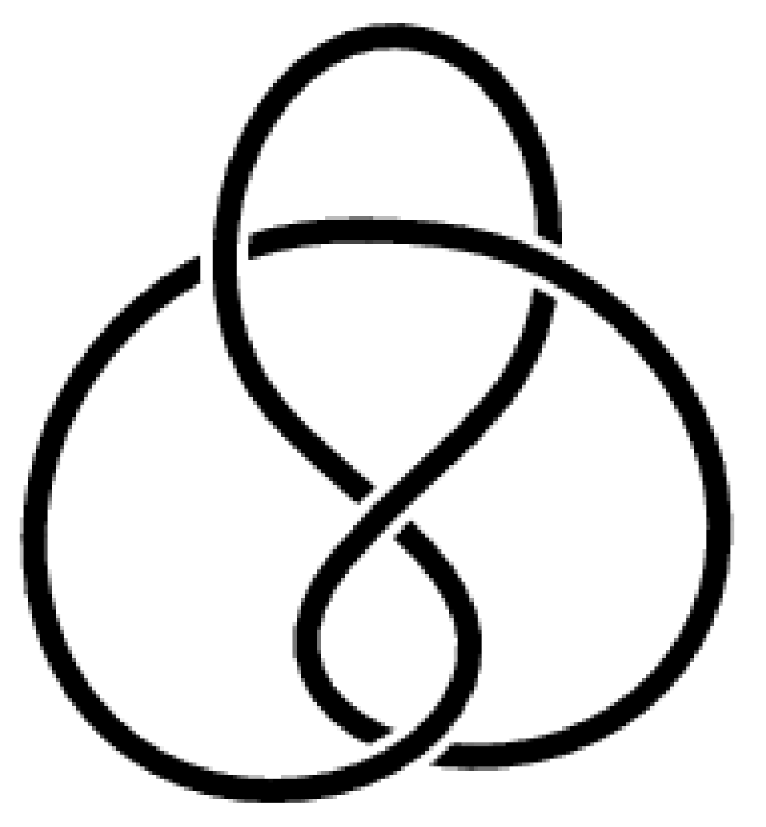
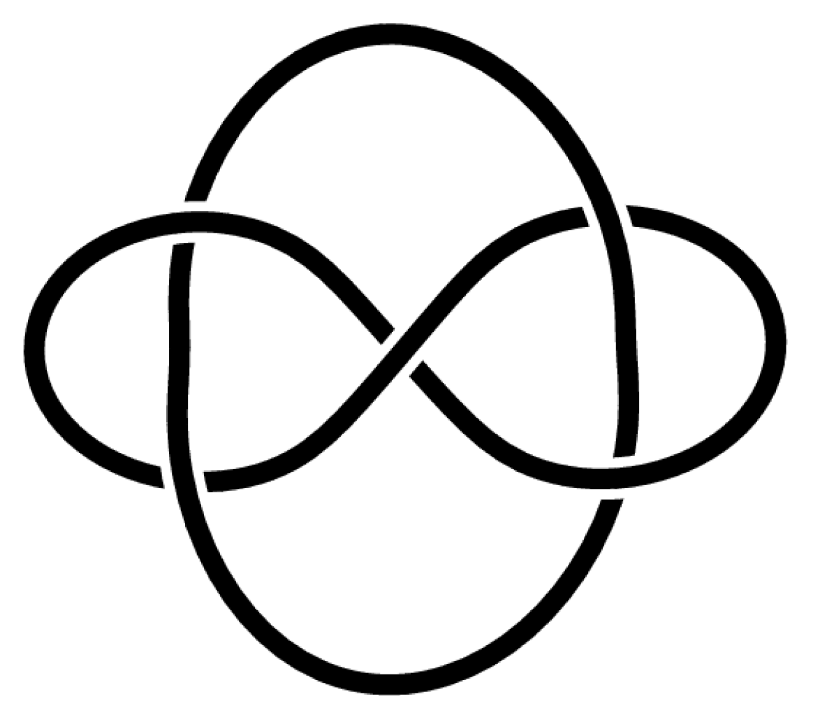
In the previous sections, we describe the knot complement of the simplest knot, the trefoil. However, there are more complicated knots. The complexity of knots is measured by the number of crossings. There is only one knot with three crossings (trefoil) and with four crossings (figure-8). For the figure-8 knot $4_1$ (see Figure 3), the knot group is given by

$${\pi }_1\left(C\left(4_1\right)\right)=\langle a,b|ba{b}^{-1}ab=ab{a}^{-1}ba\rangle$$

admitting a representation $\varphi$ into $SU\left(2\right)$, see [2].

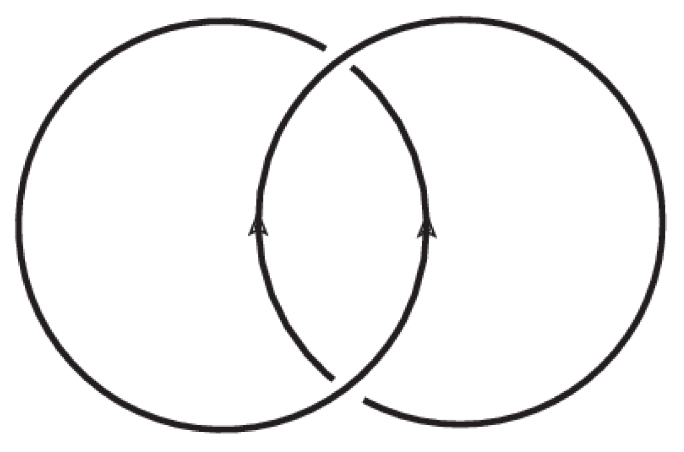
Here, we remark that the figure-8 knot is part of a large class, the so-called hyperbolic knots. Hyperbolic knots are characterized by the property that the knot complement admits a hyperbolic geometry. Hyperbolic knot complements have special properties, in particular topology and geometry are connected in a special way. We will come back to these ideas in our forthcoming work. As explained above, knot groups admit representations into $SU\left(2\right)$ leading to 1-qubit operations. Therefore, we have to change the complexity in another direction by adding more components, i.e., we have to go from knots to links. The simplest link is the Hopf link (denoted as $L2a1$, see Figure 4), the linking of two unknotted curves.

The knot group is simply

$${\pi }_1\left(C\left(L2a1\right)\right)=\langle a,b|ab{a}^{-1}{b}^{-1}=[a,b]=e\rangle =\mathbb{Z}\oplus \mathbb{Z}$$

Here, we will discuss a toy model, every component is related to a $SU\left(2\right)$ representation, i.e., the knot group ${\pi }_1\left(C\left(L2a1\right)\right)$ is represented as $SU\left(2\right)\otimes SU\left(2\right)$ via the Berry connection. Now we associate to each component of the link a representation and a generator of $SU\left(2\right)$ (i.e., ${\sigma }_x,{\sigma }_y$ or ${\sigma }_z$), say ${\sigma }_x$ to one component (the generator $a\in {\pi }_1\left(C\left(L2a1\right)\right)$) and ${\sigma }_z$ to the other component (the generator $b\in {\pi }_1\left(C\left(L2a1\right)\right)$). By using the relation between the group commutator and the Lie algebra commutator of the enveloped Lie algebra $U\left(SU\right(2\left)\right)$, we want to express the relation $[a,b]=e$ via the exponential of the commutator ${\sigma }_x\otimes {\sigma }_z-{\sigma }_z\otimes {\sigma }_x$ via the usual relation between the Lie algebra commutator and this commutator. It induces a representation

$${\pi }_1\left(C\left(L2a1\right)\right)\to SU\left(2\right)\otimes SU\left(2\right)$$

by using the exponential map $exp\left(\mathfrak{su}\right(2)\otimes \mathfrak{su}(2\left)\right)$. The relation in ${\pi }_1\left(C\left(L2a1\right)\right)$ can be expressed as Lagrangian multiplier (in the usual way) so that we get the Hamiltonian

$$H={\sigma }_x\otimes {\sigma }_z-{\sigma }_z\otimes {\sigma }_x$$

and we get the qubit operation by the exponential

$$U=exp\left(it({\sigma }_x\otimes {\sigma }_z-{\sigma }_z\otimes {\sigma }_x)\right)$$

for a suitable time t. Now we see the principle: we associate a term ${\sigma }_x\otimes {\sigma }_z$ to an over-crossing between the two components and a term ${\sigma }_z\otimes {\sigma }_x$ for the under-crossing. In the last example, we will consider the famous Whitehead link (see Figure 5).

The knot group is given by

$${\pi }_1\left(C\left(Wh\right)\right)=\langle x,y|[x,y][x,y^{-1}][x^{-1},y^{-1}][x^{-1},y]=e\rangle$$

and as described above we will associate the tensor products of the generators to the over-crossings or under-crossings between the components. Then, we will get

$$H=2{\sigma }_x\otimes {\sigma }_z-2{\sigma }_z\otimes {\sigma }_x$$

with the operation

$$U=exp\left(i2t({\sigma }_x\otimes {\sigma }_z-{\sigma }_z\otimes {\sigma }_x)\right)$$

with another choice of the time variable.

7. Discussion

In this paper, we presented some ideas to use 3-manifolds for quantum computing. A direct usage for surfaces (related to anyons) is not possible, but we explained above that the best representative is the fundamental group of a manifold. The fundamental group is the set of closed curves up to deformation with concatenation as group operation (also up to deformation). Every 3-manifold can be decomposed into simple pieces so that every piece carries a geometric structure (out of eight classes). In principle, the pieces consist of complements of knots and links. Then, the fundamental group of the knot complement, known as knot group, is an important invariant of the knot or link. Why not use this knot group for quantum computing? In [3,4,22,23], M. Planat et al. studied the representation of knot groups and the usage for quantum computing. Here, we discussed a direct relation between the knot complement and quantum computing via the Berry phase. The knot group determines the operations where we fix a suitable $SU\left(2\right)$ representation. As a result, we get all 1-qubit operations for a knot. Then, we discussed the construction of 2-qubit operations by the linking of two knots. The concrete realization of these ideas by a device will be shifted to our forthcoming work.

References

- Wang, Z. Topological Quantum Computation; Regional Conference Series in Mathematical/NSF-CBMS; AMS: Providence, Rhode Island, 2010; Volume 112. [Google Scholar]
- Kirk, P.; Klassen, E. Chern-Simons invariants of 3-manifolds and representation spaces of knot groups. Math. Ann. 1990, 287, 343–367. [Google Scholar] [CrossRef]
- Planat, M.; Aschheim, R.; Amaral, M.; Irwin, K. Universal quantum computing and three-manifolds. Symmetry 2018, 10, 773. [Google Scholar] [CrossRef] [Green Version]
- Planat, M.; Aschheim, R.; Amaral, M.; Irwin, K. Quantum computing, Seifert surfaces and singular fibers. Quantum Rep. 2019, 1, 3. [Google Scholar] [CrossRef] [Green Version]
- Kauffman, L. Knots and Physics; Series on Knots and Everything; World Scientific: Singapore, 1994; Volume 1. [Google Scholar]
- Kauffman, L. Knot Logic. In Knots and Applications; Kauffman, L., Ed.; Series on Knots and Everything; World Scientific: Singapore, 1995; Volume 6, pp. 1–110. [Google Scholar]
- Kauffman, L. Knots. In Geometries of Nature, Living Systems and Human Cognition: New Interactions of Mathematics with Natural Sciences and Humanities; World Scientific: Singapore, 2005; pp. 131–202. [Google Scholar]
- Boi, L. Topological Knot Models. In Geometries of Nature, Living Systems and Human Cognition: New Interactions of Mathematics with Natural Sciences and Humanities; World Scientific: Singapore, 2005; pp. 203–278. [Google Scholar]
- Baez, J. Higher-dimensional Algebra and Planck-scale Physics. In Physics Meets Philosophy at the Planck Scale; Callender, C., Huggett, N., Eds.; Cambridge University Press: Cambridge, UK, 2001; pp. 177–195. [Google Scholar]
- Bilson-Thompson, S.; Markopoulou, F.; Smolin, L. Quantum Gravity and the Standard Model. Class. Quant. Grav. 2007, 24, 3975–3994. [Google Scholar] [CrossRef]
- Gresnigt, N. Braids, Normed Division Algebras, and Standard Model Symmetries. Phys. Lett. B 2018, 783, 212–221. [Google Scholar] [CrossRef]
- Asselmeyer-Maluga, T. Braids, 3-Manifolds, Elementary Particles: Number Theory and Symmetry in Particle Physics. Symmetry 2019, 11, 1298. [Google Scholar] [CrossRef] [Green Version]
- Milnor, J. A unique decomposition theorem for 3-manifolds. Amer. J. Math. 1962, 84. [Google Scholar] [CrossRef]
- Jaco, W.; Shalen, P. Seifert Fibered Spaces in 3-Manifolds; Academic Press: Cambridge, MA, USA, 1979; Volume 21. [Google Scholar]
- Thurston, W. Three-Dimensional Geometry and Topology, 2nd ed.; Princeton University Press: Princeton, NJ, USA, 1997. [Google Scholar]
- Gordon, C.; Luecke, J. Knots are determined by their complements. J. Am. Math. Soc. 1989, 2, 371–415. [Google Scholar] [CrossRef]
- Rolfson, D. Knots and Links; Publish or Prish: Berkeley, CA, USA, 1976. [Google Scholar]
- Prasolov, V.; Sossinisky, A. Knots, Links, Braids and 3-Manifolds; AMS: Providence, RI, USA, 1997. [Google Scholar]
- Kauffman, L.; Lomonaco, S. Topological quantum computing and SU(2) braid group representations. In Proceedings of the SPIE 6976, Quantum Information and Computation VI, 69760M, Orlando, FL, USA, 24 March 2008; The International Society for Optical Engineering: Bellingham, WA, USA, 2008; Volume 6976. [Google Scholar] [CrossRef]
- Milnor, J. On the existence of a connection with curvature zero. Comment. Math. Helv. 1958, 32, 215–223. [Google Scholar] [CrossRef] [Green Version]
- Zu, C.; Wang, W.B.; He, L.; Zhang, W.G.; Dai, C.Y.; Wang, F.; Duan, L.M. Experimental Realization of Universal Geometric Quantum Gates with Solid-State Spins. Nature 2014, 514, 72. [Google Scholar] [CrossRef] [PubMed] [Green Version]
- Planat, M.; Zainuddin, H. Zoology of Atlas-Groups: Dessins d’enfants, Finite Geometries and Quantum Commutation. Mathematics 2017, 5, 6. [Google Scholar] [CrossRef] [Green Version]
- Planat, M.; Ul Haq, R. The Magic of Universal Quantum Computing with Permutations. Adv. Math. Phys. 2017, 2017, 5287862. [Google Scholar] [CrossRef] [Green Version]
Figure 1.
The simplest knot, trefoil knot .
Figure 2.
Generators (red circle) of knot group for trefoil .
Figure 3.
figure-8 knot .
Figure 4.
Hopf link .
Figure 5.
Whitehead link .
Publisher’s Note: MDPI stays neutral with regard to jurisdictional claims in published maps and institutional affiliations. |
© 2021 by the author. Licensee MDPI, Basel, Switzerland. This article is an open access article distributed under the terms and conditions of the Creative Commons Attribution (CC BY) license (http://creativecommons.org/licenses/by/4.0/).
Share and Cite
MDPI and ACS Style
Asselmeyer-Maluga, T. Topological Quantum Computing and 3-Manifolds. Quantum Rep. 2021, 3, 153-165. https://0-doi-org.brum.beds.ac.uk/10.3390/quantum3010009
AMA Style
Asselmeyer-Maluga T. Topological Quantum Computing and 3-Manifolds. Quantum Reports. 2021; 3(1):153-165. https://0-doi-org.brum.beds.ac.uk/10.3390/quantum3010009
Chicago/Turabian StyleAsselmeyer-Maluga, Torsten. 2021. "Topological Quantum Computing and 3-Manifolds" Quantum Reports 3, no. 1: 153-165. https://0-doi-org.brum.beds.ac.uk/10.3390/quantum3010009