Seasonal and Inter-Annual Variability of the Phytoplankton Dynamics in the Black Sea Inner Basin


1
Joint Research Centre (JRC), European Commission, 21027 Ispra, Italy
2
Instituto de Ciencias Marinas de Andalucía (ICMAN), Consejo Superior de Investigaciones Científicas (CSIC), 11510 Puerto Real, Spain
*
Author to whom correspondence should be addressed.
Oceans 2020, 1(4), 251-273; https://0-doi-org.brum.beds.ac.uk/10.3390/oceans1040018
Submission received: 18 August 2020
/
Revised: 13 October 2020
/
Accepted: 14 October 2020
/
Published: 20 October 2020
(This article belongs to the Special Issue Current Advances and Challenges in Ocean Science—Feature Papers for the Founding of Oceans)
Abstract
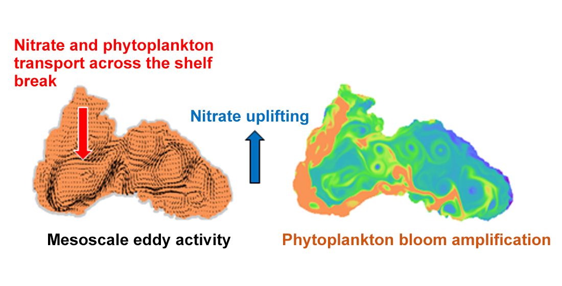
:We explore the patterns of Black Sea phytoplankton growth as driven by the thermohaline structure and circulation system and the freshwater nutrient loads. Seasonal and inter-annual variability of the phytoplankton blooms is examined using hydrodynamic simulations that resolve mesoscale eddies and online coupled bio-geochemical model. This study suggests that the bloom seasonality is homogeneous across geographic locations of the Black Sea inner basin, with the strongest bloom occurring in winter (February–March), followed by weaker bloom in spring (April–May), summer deep biomass maximum (DBM) (June–September) and a final bloom in autumn (October–November). The winter phytoplankton bloom relies on vertical mixing of nitrate from the intermediate layers, where nitrate is abundant. The winter bloom is highly dependent on the strength of the cold intermediate layers (CIL), while spring/summer blooms take advantage of the CIL weakness. The maximum phytoplankton transport across the North Western Shelf (NWS) break occurs in September, prior to the basin interior autumn bloom. Bloom initiation in early autumn is associated with the spreading of NWS waters, which in turn is caused by an increase in mesoscale eddy activity in late summer months. In summary, the intrusion of low salinity and nitrate-rich water into the basin interior triggers erosion of the thermocline, resulting in vertical nitrate uplifting. The seasonal phytoplankton succession is strongly influenced by the recent CIL disintegration and amplification of the Black Sea circulation, which may alter the natural Black Sea nitrate dynamics, with subsequent effects on phytoplankton and in turn on all marine life.

1. Introduction
Phytoplankton blooms [1] are identifiable signals of the annual growth activity in pelagic systems. Typical Black Sea seasonal phytoplankton dynamics are characterised by a major phytoplankton bloom in winter (February) followed by a smaller spring (March–April) bloom [2,3,4,5]. It has been found that windy, cold winters lead to an abundance of phytoplankton biomass (PHY) or chlorophyll-a (CHLa) concentrations in winter-spring, due to enhanced vertical mixing and stronger upwelling. Thus, the inter-annual variability of phytoplankton blooms has been associated with the winter severity. In summer the phytoplankton growth on the surface decays because of nitrate depletion, and autumn bloom follows between September and November. During the late autumn and winter-spring blooms, PHY reaches a maximum in the upper mixed layer. From June to October, the maximum of PHY (so-called DBM) appears at the subsurface layer, associated with the uppermost pycnocline. The February–April blooms are clearly detected by both types of CHLa measurement modalities used: in-situ and satellite [2,5,6]. Satellite data showed that the autumn blooms are more abundant than the spring blooms. The trend towards milder winters has been cited as the reason for the disappearance of the spring bloom in the open Black Sea [7]. It has been assumed that in years with temperatures in line with the inter-annual average, CHLa peaks in winter and the spring peak is absent, whereas in cold years, the relatively low CHLa in winter is followed by a spring bloom. Specifically, a decrease in the frequency of cold winters results in changes in the timing of the winter-early spring bloom, which either weakened or disappeared altogether depending on local meteorological and oceanographic conditions [5]. It is believed that the open Black Sea experiences a bloom cycle with an autumn CHLa peak and summer minimum, but no spring bloom on the surface in an atypical year [8]. Several authors suggested a possible relationship between cold intermediate layers (CIL) thickness and phytoplankton blooms [5,6,8]. There is an established intensification of the autumn blooms over the last 20 years [9]. In general, there is no clear consensus in the literature concerning the exact seasonality of PHY/CHLa dynamics observed in the Black Sea.
The inconsistency between measurements is noticeable when comparing in-situ and remote sensing studies in the Black Sea. For example, it is suggested that CHLa density is overestimated for the open sea by up to a factor of four, when computed using the global SeaWiFS chlorophyll model, when compared to direct in-situ measurements [10]. The difference between satellite-based estimates and in-situ measurements is even larger for the coastal regions [11]. The analysis of MODIS-Aqua data for 2003–2013 and SeaWiFS data for 1998–2007 indicates that Oceancolor Level 2 and 3 chlorophyll data contain systematic inconsistencies in the Black Sea basin, which are related to the effect of cloud shadows [12]. In summary, the seasonal CHLa density estimation from satellite observations appears to be less reliable for the Black Sea, and consequently so are the conclusions for seasonal phytoplankton and inter-annual evolution in the literature, which are solely based on satellite data.
During the last two decades, the Black Sea ecosystem evolution has been studied by using a variety of models with different levels of complexity [13,14,15,16]. Even though the existing studies have provided deep knowledge on the Black Sea plankton dynamics and certain important North Western Shelf (NWS) processes, the current understanding of the mechanisms that control the seasonality and magnitude of the phytoplankton blooms is still incomplete.
The impact of mesoscale (or sub-mesoscale) physics on both hydrodynamics and phytoplankton production has been discussed [17,18]. The largest mesoscale eddies (MEs) in the Black Sea emerge from instabilities of horizontally sheared motions, particularly in the boundaries of the Rim Current. The MEs appears to be a possible mechanism for offshore transport of nutrients. The distribution of hydro-chemical properties in the upper layer seems to be sensitive to external pressures originating from regional weather variability [19,20] and anthropogenic inputs [21,22]. It is important to recognise the contribution of the mesoscale circulations in supporting offshore phytoplankton production. In addition, the ability of nutrient-rich NWS waters to enhance phytoplankton blooms should be evaluated.
The present study motivation is to address the gaps in the literature regarding forcing and dynamics of plankton seasonality in the basin of the Black Sea. To achieve this goal, the study exploits a previously developed hydrodynamic model to perform reliable long-term simulations of the Black Sea dynamics [23]. The paper aims to explore the seasonality and inter-annual variation of the phytoplankton bloom in the Black Sea inner basin. The effect of CIL thickness and temperature on seasonal phytoplankton blooms is studied in detail. We examine the dynamics of the Black Sea surface circulation system and cross-shelf transport to propose a mechanism of initiation of the early autumn bloom.
2. Methods and Data
2.1. Geographical Area of Interest
When identifying the sources and levels of nitrate, the Black Sea basin can be divided into two main parts. One part includes the NWS and South Western Self (SWS), which receive nitrate coming from the Danube and other big rivers flowing into the NWS during a large part of the year. It is assumed that phosphate is limiting the phytoplankton growth in these regions, due to excess of inorganic nitrogen exceeding the stoichiometric amount of phosphate [19]. In the rest of the Black Sea, however, nitrate is the limiting nutrient for phytoplankton growth [11]. The nitrate concentration is less than 0.1 mmol N m−3 in the surface waters of the inner sea for most of the year except for periods of strong vertical winter mixing and infrequent intrusion from coastal regions [24,25]. The euphotic zone in the Black Sea interior typically extends to a depth of about 30–45 m [26], in which the concentration of oxygen is high (more than 100 mmol O2 m−3), while nutrients and organic matter concentrations vary seasonally [25]. The depth distribution profile of nitrate is characterised by a subsurface maximum located below the euphotic zone (~55 m depth), following a rapid decrease of nitrate with increasing depth, and absence of nitrate in the deep sea. That intermediate layer (located between 30–150 m depth) containing a high concentration of nitrate (0.5–5 mmol N m−3) is called the nitrate storage henceforth.
The accumulation of nitrate in intermediate water layers can be explained by its production, namely, nitrification and remineralisation, as well as the very slow uptake rates. It is further assumed that there are external sources of nitrate contributing to the inner basin concentration, such as river-based and atmospheric input. For instance, 20% of nitrates consumed by phytoplankton in the open waters are of allochthonous origin [27]. Moreover, based on satellite observation, it is thought that anthropogenic forces on the NWS shelf did not significantly influence the ecosystem of the deep part of the Black Sea during the 1970s to mid-1980s [21].
The Black Sea is characterised by large spatial heterogeneity of bio-hydro-chemical characteristics [19,23,28]. The main processes governing nutrient spreading are large-scale horizontal currents and mesoscale eddy fields, in conjunction with vertical turbulent mixing during phases of convection in winter. One general hypothesis is the strengthening of the basin-scale cyclonic circulation in winter and the intensification of anticyclone activity in the warm summer–autumn months [23,29,30]. Typically, in late summer and early autumn, an abundance of anticyclonic eddies is formed between the shelf edge and the Rim Current.
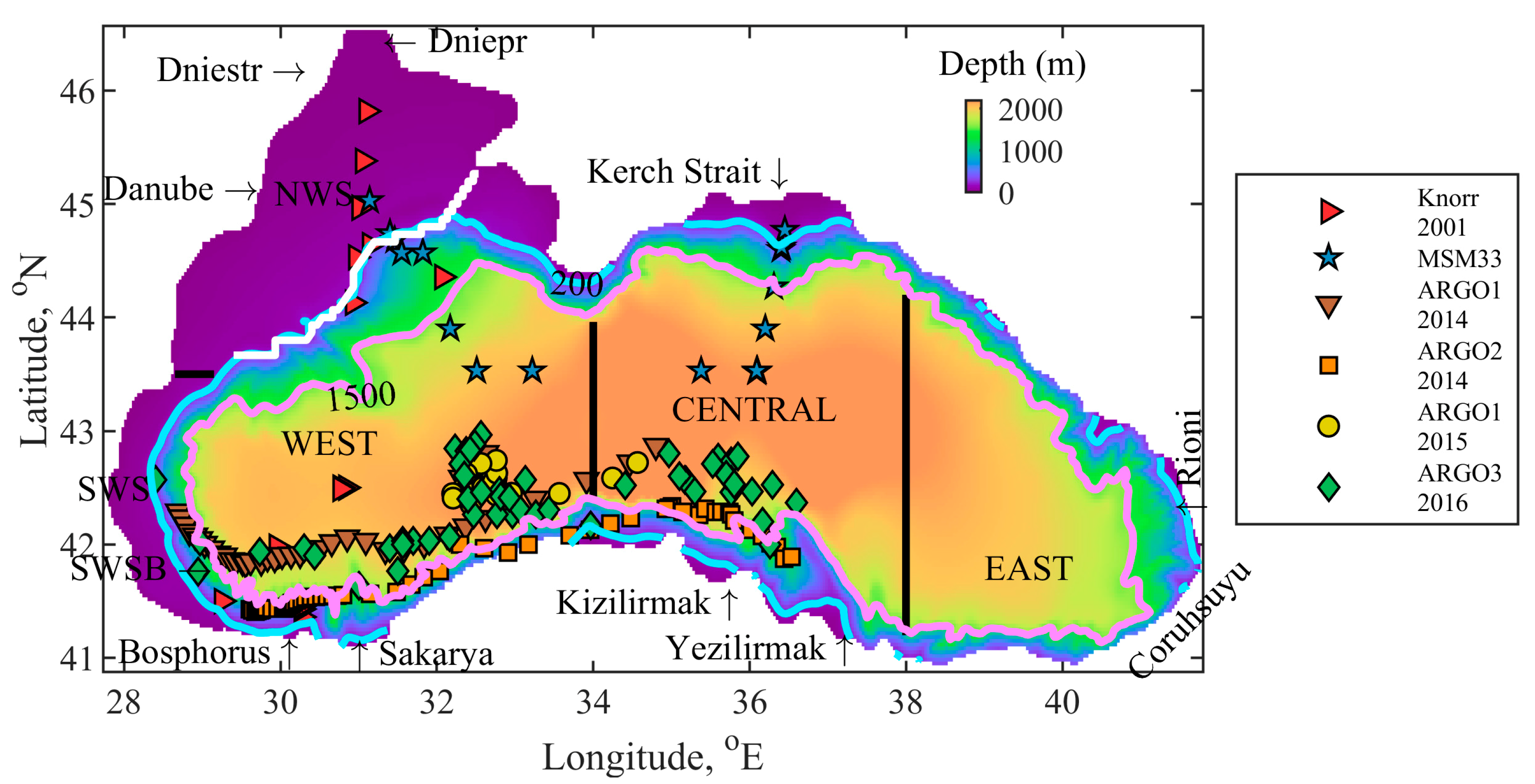
We consider three deep regions: The deep basin, of depth greater than 1500 m, is divided into three regions (WEST, CENTRAL and EAST). The basin separation is introduced for model validation purposes. It is assumed that the layer located between 200 and 1500 m in depth covers the shelf-break (SB) and continental slope. The southern and south-western shelf-break areas (SWSB) comprise the southern part of this strip. The NWS is less than 200 m deep and is located above 43.5° N, while the SWS is the area below 43.5° N. This study is focused on the phytoplankton succession in the inner Black Sea basin (limited by the 1500 m isobath in Figure 1).
2.2. Hydrodynamic Model
A hydrodynamic model, which represents the mesoscale circulations and thermohaline structure in the Black Sea for a continuous multi-decadal period, without any relaxation towards external fields, is used for this study [23]. This 3D hydrodynamic model involves two modules: GETM [31] and GOTM. It is initialised on a high resolution 2 × 2 min latitude–longitude horizontal grid. The meteorological forcing from the European Centre for Medium Range Weather Forecast (ECMWF) [32], based on 6-hourly records, has been applied (ERA-Interim project). Monthly mean freshwater input has been estimated using the values from the Global Runoff Data Centre (GRDC) runoff [33]. The model is initialised using temperature and salinity 3D fields coming from the MEDAR/MEDATLAS II project [34]. The 3D hydrodynamic model has been successfully applied to study the long term (1960–2015) thermohaline structure and circulation in the Black Sea previously [23,35].
2.3. Lower Trophic Level Model
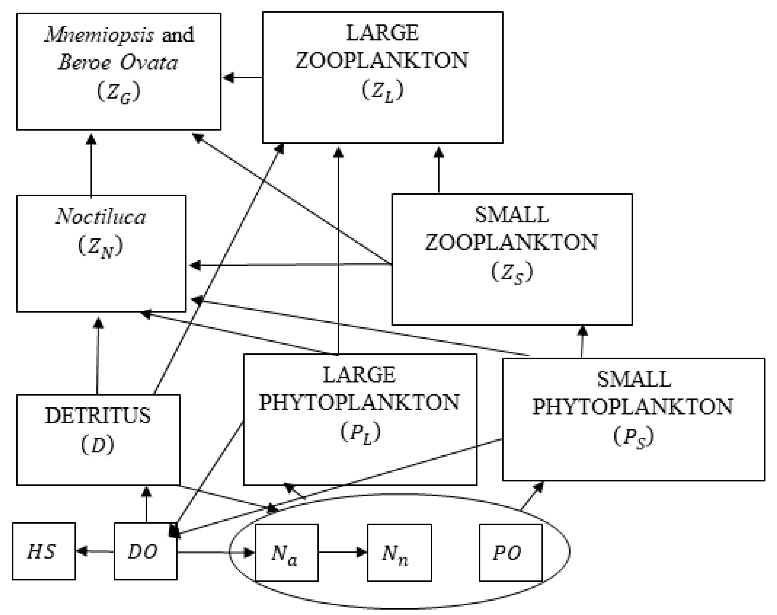
The flow fields from the hydrodynamic model are used to predict the evolution of the low trophic level components of the food chain in the Black Sea ecosystem [36]. A nitrate-based biogeochemical model has been implemented, taking inspiration from the models already existing in the literature [37,38]. The model is purposefully adapted for the Black Sea basin, where a unique ecosystem exists. It represents the classical omnivorous food-web with 12 state variables (Figure 2). These include two phytoplankton size groups–small (PS) and large (PL), four zooplankton groups, including micro and meso-zooplankton (ZS and ZL), non-edible dinoflagellate species as Noctiluca (ZN) and gelatinous zooplankton species Mnemiopsis and Beroe Ovata (ZG). All plankton biomasses are expressed in nitrogen units, since nitrogen is considered to be the most important limiting nutrient for the interior Black Sea ecosystem [39]. Nitrogen is represented by two inorganic nutrients—nitrate (Nn) and ammonium (Na) and is included in the particulate organic material—detritus (D). The Black Sea Ecosystem Model (BSEM) model is further modified in Reference [40] where the phosphate (PO) state variable is added in order to consider phosphorus as limiting the phytoplankton production rate together with nitrogen and photosynthetically available radiation. Other state variables incorporate dissolved oxygen (DO) and hydrogen sulphide (HS). The values of the coefficients in the BSEM model equations are obtained either from the literature or from fitting the model to measured concentration profiles in the Black Sea basin. Nevertheless, the updated BSEM parameters (Tables S1 and S2) do not differ substantially from their original values [38]. The Supplementary file includes all model equations describing the evolution of the state variables and the values of model parameters.
River nutrient load data is issued from the SESAME and PERSEUS projects [41]. It consists of systematic nutrient measurements at the Danube discharge sections from the 1990s until 2008. Climatological mean Danube nutrient loads (averaged over the 1990–2008 period) are used from the beginning of 2009 for the Danube. For the other model rivers (Figure 1) data is not available since the 1990s, thus, climatological mean data is used in all cases to fill in the gaps. Model sensitivity analysis shows that initial nutrient concentration in the intermediate and deep layers is a very important part of the model setup, since it can support phytoplankton growth, even without loading from the rivers. Thus, the nutrient climatology for the Black Sea, coming from [34], is used as initial conditions for nitrate, ammonium and phosphate. This dataset reflects the main features known from observations, such as the existence of the intermediate layer in the basin interior of high nitrate concentration (nitrate storage) [25,42]. At depths greater than 115 ± 15 m, ammonium, phosphate and hydrogen sulphide concentrations increase. Hydrogen sulphide is zero in the upper 90 m, and then increases linearly to 500 mmol HS m−3 at the seabed level. Dissolved oxygen decreases linearly from 340 mmol O2 m−3 to 0 in the upper 150 m and is set to zero further below [43,44]. All other BSEM model state variables are set to 0.0225 mmol N m−3 and vertically uniformity over the entire water column is assumed. This assumption is based on the fact that equilibrium structures do not depend on the initial conditions and are emergent properties of the model dynamics. A comparison of the atmospheric and riverine inputs for the Black Sea revealed that atmospheric-dissolved, inorganic nitrogen ranged between 4% and 13% of the total inorganic nitrogen, while the atmospheric-dissolved, inorganic phosphorus fluxes had significantly higher contributions with values ranging from 12% to 37% of the total inorganic phosphorus [45]. According to Reference [46], the atmospheric input of oxidised nitrogen can reach 13% of the total inorganic nitrogen input of the Danube. Such a flux can sustain up to 15% of the new phytoplankton production. We considered constant atmospheric surface fluxes of 0.083 mmol N m−2d−1 nitrate, 0.0225 mmol N m−2d−1 ammonium, and 0.0052 mmol P m−2d−1 phosphate. These values are in close agreement with the lower bounds of the experimental data presented in Reference [45].
The issue of what constitutes a bloom is more than a biomass issue [1]. It is assumed in Reference [47] that the total carbon biomass of non-blooming events was normally distributed with a seasonal mean described by a periodic spline function. Blooms were identified as significant deviations above this pattern. In this study, we use a criterion for the bloom definition by considering an occurrence of a bloom when the actual PHY (chlorophyll-a concentration) in the basin is larger than the mean average for the entire analysed period. We are not dealing merely with the exponential growth part of the phytoplankton curve, but are looking at the long-term, seasonal dynamic of that curve.
PHY (mg C m−3) is calculated as the sum of small and large phytoplankton, which is converted from mmol N m−3 to mg C m−3 using the 6.625 Redfield ratio. Then, in order to compare with observational data, the stoichiometric conversion of mmol N m−3 to mg CHLa m−3 is done. Despite the existing underlying complexity of this conversion [48,49], the last ratio is usually taken as a constant, which is assumed to be 1 [13,14,50].
2.4. Model Validation Statistics
Model validation statistics used in this study are the average absolute error (AAR) and Pearson correlation coefficient (R), displayed with their 95% confidence intervals. Model skills (Mskill) are evaluated using root mean square error (RMSE) and standard deviation (std), namely:
A value close to one indicates a close match between observations and model prediction. A value close to zero indicates that the mechanistic model has the poor predictive capacity and performs, as well as a simple, data-driven statistical model would. Values inferior to zero indicate that the observation means would be a better predictor than the mechanistic model results. Statistical measures, such as the normalised root mean squared difference (RMSD) and normalised standard deviation (model statistics are divided by the observational ones) are used in Section 3 for model validation (Taylor diagram).
2.5. Validation Data
Several different CHLa datasets of the Black Sea surface and water column are used in this study (Table 1). The Copernicus dataset is averaged and reprocessed with the BSAlg algorithm [51]. TheRegAlg time series of CHLa from 1999 to 2008 are redrawn from Reference [4]. In-situ vertical profiles of CHLa were collected during the R/V Knorr 2001 research cruise to the Black Sea (23 May to 10 June 2001). The station locations for the R/V Knorr 2001 are shown in Figure 1. They are well situated to study WEST, SWSB, and NWS-SB regions of the Black Sea [52]. Refer to Figure 1 for the location of the regions of interest. MSM33 denotes sampling conducted from the 11 November to the 2 December 2013 during cruise 33 of the German R/V Maria S. Merian [53]. The cruise itinerary covered the north-western and north-eastern shelf-break and the central deep Black Sea (Figure 1). In-situ vertical profiles of CHLa from the profiling float PROVOR II (ARGO) is available several (three to ten) times a month from 2014 to 2016 [54]. Locations of ARGO’s data stations can be seen in Figure 1, while the time coverage is given in Table 1.
3. Validation of the Phytoplankton Distribution Model
3.1. Validation against In-Situ Vertical Profile Data
As introduced above, the study focuses on the phytoplankton bloom dynamics and the physical factors governing its life cycle in the Black Sea inner basin. Before addressing this topic, we assess the model’s ability to capture the amplitudes and phases of known seasonal blooms, as well as CHLa seasonal cycles for the different study areas, located in the Black Sea basin. The in-situ measurements are used to assess the deep CHLa maximum (DCM) over a short period of time, although the data coverage from in-situ observations remains sparse in the Black Sea.
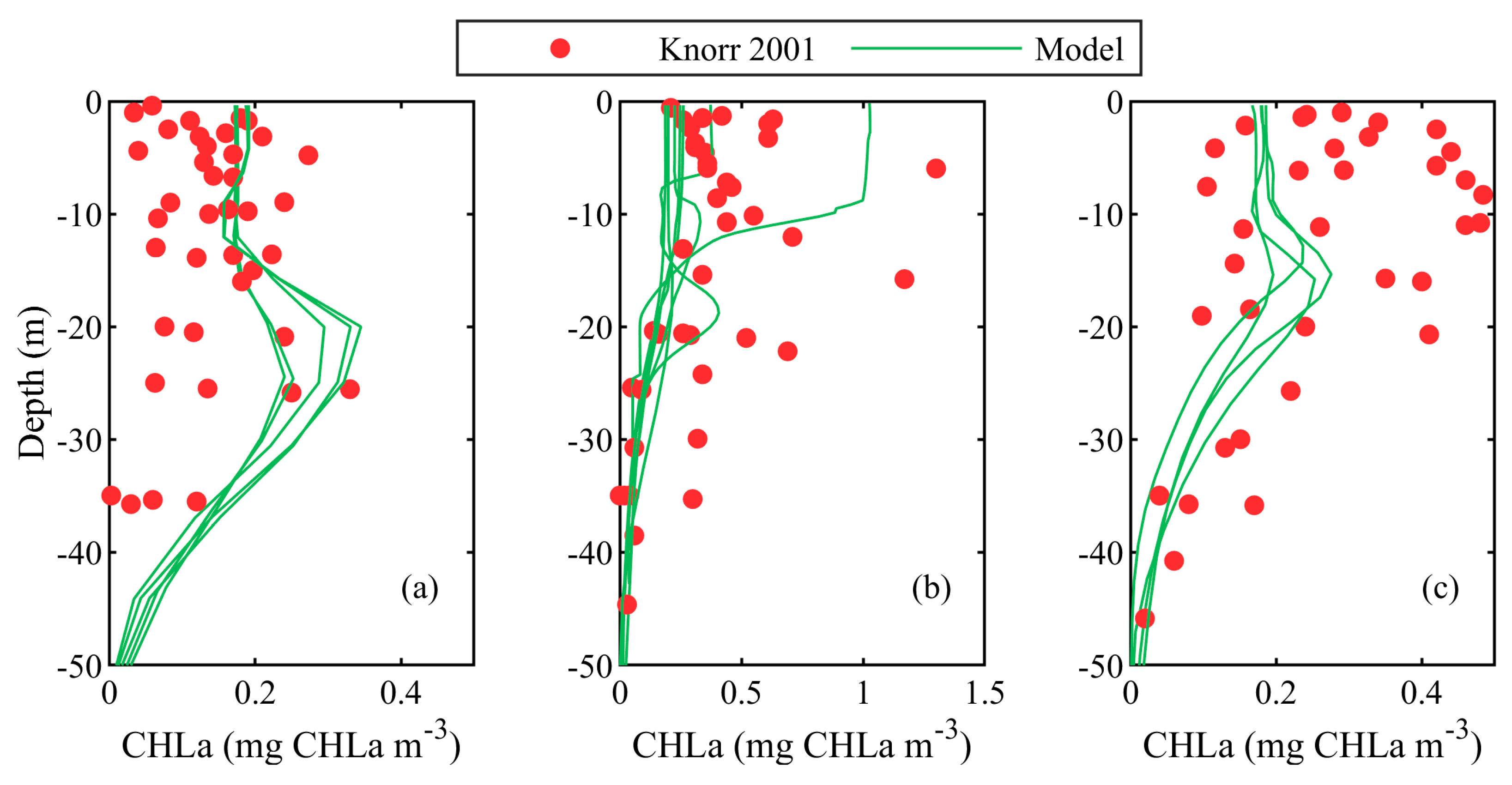
A comparison between the Knorr 2001 CHLa (mg CHLa m−3) vertical profiles and the modelled CHLa (mg CHLa m−3) concentrations are shown in Figure 3. Based on different hydrodynamic conditions, the vertical CHLa profiles are sorted into three groups, namely, for WEST, SWSB and NWS-SB. This categorisation is necessary because a few CHLa samples exist in each of these areas (locations of the sample stations are marked with red symbols in Figure 1). There is no data for the CENTRAL, EAST or SWS regions. In the WEST Black Sea waters (Figure 3a), the CHLa concentration profile exhibits a quasi-regular change below the thermocline, where the CHLa value increases to a maximum below the surface and then sharply decreases to zero. Hardly any abundance of CHLa is predicted by our model below 50 m depth, in accordance with in-situ data [2]. Our model results suggest a local maximum at about 20–25 m depth, while the in-situ data shows a maximum at about 15–20 m. In the NWS-SB area, the empirically measured CHLa profiles (Figure 3b) show a lack of obvious pattern: No noticeable maximum, a uniform concentration in the upper 20 m, and then a systematic decrease to zero. Our CHLa vertical profiles are in good agreement with the observational data in the aforementioned studies. In Figure 3c, are shown vertical CHLa profiles for the Knorr 2001 measurements, gathered by stations located in the SWSB. This is a hydrodynamically dynamic area, which is strongly influenced by the Rim Current speed. The DCM modelled by the BSEM is located at 20 m below the surface, while the measured DCM oscillates between 10 and 20 m below the surface. The individual CHLa model results from the three areas (WEST, NWS-SB and SWSB) are compared with the corresponding Knorr 2001 data in Figure 4a in the shape of a Taylor diagram. The best correlation is found for NSW-SB area, where the correlation coefficient is ~0.85, and the normalised RMSD is the lowest. Because of the limited amount of Knorr 2001 data, the model performance is evaluated over the merged datasets. In particular, the AAE = 0.151 ± 0.034 mg CHLa m−3 and . The discrepancy between our model and observed values is small, and the correlation between them is moderate, Mskill is greater than zero, which tells us that the model can describe the average empirical CHLa vertical profile. Figure 4b shows the comparison between MSM33 surface CHLa and modelled surface CHLa concentration. The correlation is good, yet the calculated values are lower than both in-situ measurements. A possible explanation includes the assumed N:CHLa ratio in this study.
3.2. Validation against Remote Sensing Data
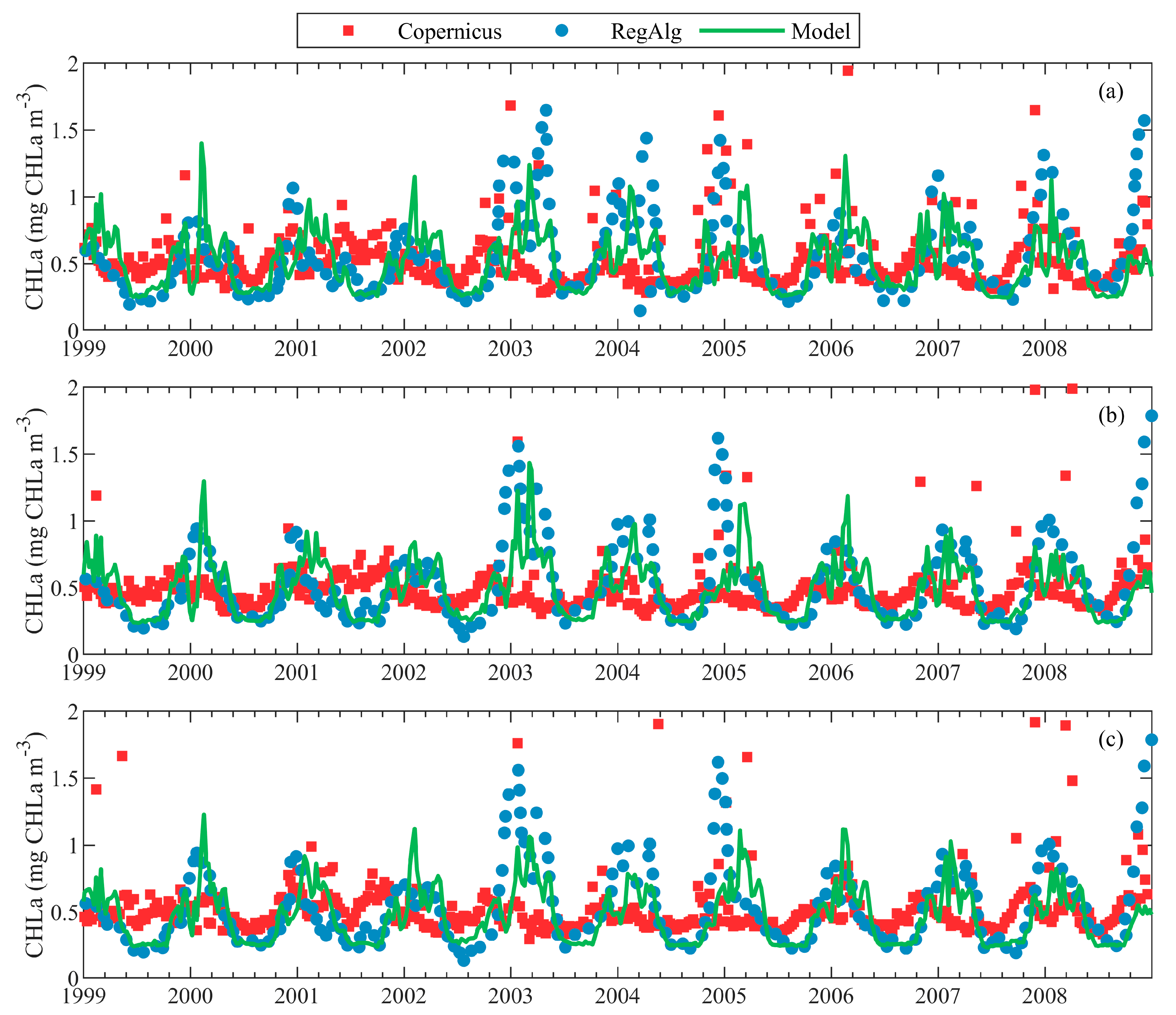
In Figure 5, we compare different surface CHLa datasets for the period 1999–2008. The time period is chosen to correspond to the RegAlg data availability. BSEM model results are compared with two data sets based on satellite observations. We decided to compare eight-day mean surface values of the CHLa because the most important events in the seasonal phytoplankton succession, such as blooms, often occur over a short time period, on the time scale of a week. The AAE and R coefficients, quantifying similarities between different time series are presented in Table 2. The agreement between the BSEM model and RegAlg survey is the highest, while there is no correspondence with the Copernicus survey data. This is not surprising because both satellite datasets disagree completely on the frequency and amplitude of the blooms. Interestingly, an agreement between BSEM and RegAlg in the CENTRAL Black Sea region is best. Modelled bloom amplitudes in WEST and CENTRAL regions are of the same magnitude, while in the EAST they are slightly smaller. When analysing CHLa seasonality in the three different regions, we can conclude that patterns are similar across different regions of the Black Sea. More details about PHY seasonal and inter-annual variability in the entire inner basin are given in Section 4.1 and Section 4.2.
3.3. Model Validation against Argo Floats Empirical Data
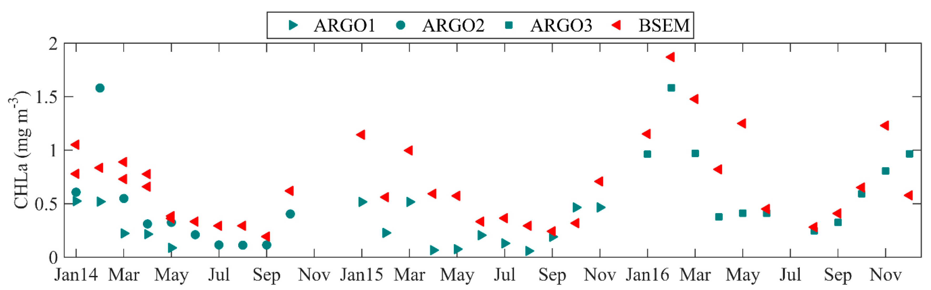
The high spatial and temporal coverage of satellite observations makes them extremely suitable for testing model simulations. However, it is clear from the above results that using only satellite CHLa data to validate model estimates has its limitations. Model validation requires comparisons with in-situ observations, too. Now, we focus on the comparison between the CHLa concentration, as measured by the ARGO floats and computed by the BSEM model. For this reason, simulated daily CHLa values are extracted at the ARGO locations (Figure 1) and averaged for the upper 5 m Black Sea depth. Then, results for all datapoints in a month are further averaged temporally. ARGO-floats acquired measurements are also averaged monthly. Comparison of the BSEM forecast with in-situ data of ARGO1, 2 and 3 (Table 1) is presented in Figure 6. The ARGO1 starts its water trajectory in January 2014 from the western shelf-break (Figure 1). Until November, the float crosses the WEST region, and reaches the CENTRAL Black Sea region in December. The ARGO2 float travels along Anatolian coast, through southern shelf-break. In 2015 the ARGO1 resided almost entirely in the WEST region, while the ARGO3 trajectory for 2016 covers the SWSB, WEST and CENTRAL regions. In all considered regions, the surface CHLa profile has a U-shape, with a maximum in winter and minimum in summer. This finding is clearly evident in both the ARGO floats data and in the BSEM model forecast. We find that the similarities between the BSEM model results and ARGO data remarkable, because during 2014–2016 the model is constrained only with climatological nutrient data for all considered rivers. Moreover, the model parameters are calibrated to capture the long-term ecosystem evolution rather than to represent a particular year, and the model is not related to any external data during the entire model run. The BSEM model was not calibrated to represent the specifics of the taxonomic composition that occur in a given year, however it has capabilities to correctly identify the overall phytoplankton patterns on both a yearly and long-term basis. Finally, the statistical analysis performed for the merged ARGO time series and corresponding BSEM model outputs indicates AAE = 0.31 ± 0.08 mg CHLa m−3, R = 0.86 (0.74, 0.93) and Mskill = 0.42.
4. Results
4.1. Seasonal Variability of PHY
We consider herein a year as ‘cold’ when the Black Sea’s winter (December–March) surface temperature (SST) in the inner basin (with depth > 1500 m) is less than the long-term mean winter SST, 8.3 °C [23]. On the contrary, when the winter SST is equal to or greater than 8.3 °C, the year is considered as ‘warm’. So, for the current simulation period, considering 1998 to 2017, the years 1998, 2000, 2002–2006, 2008, 2012 and 2017 are considered ‘cold’ (10 years) and the rest ‘warm’ (10 years).
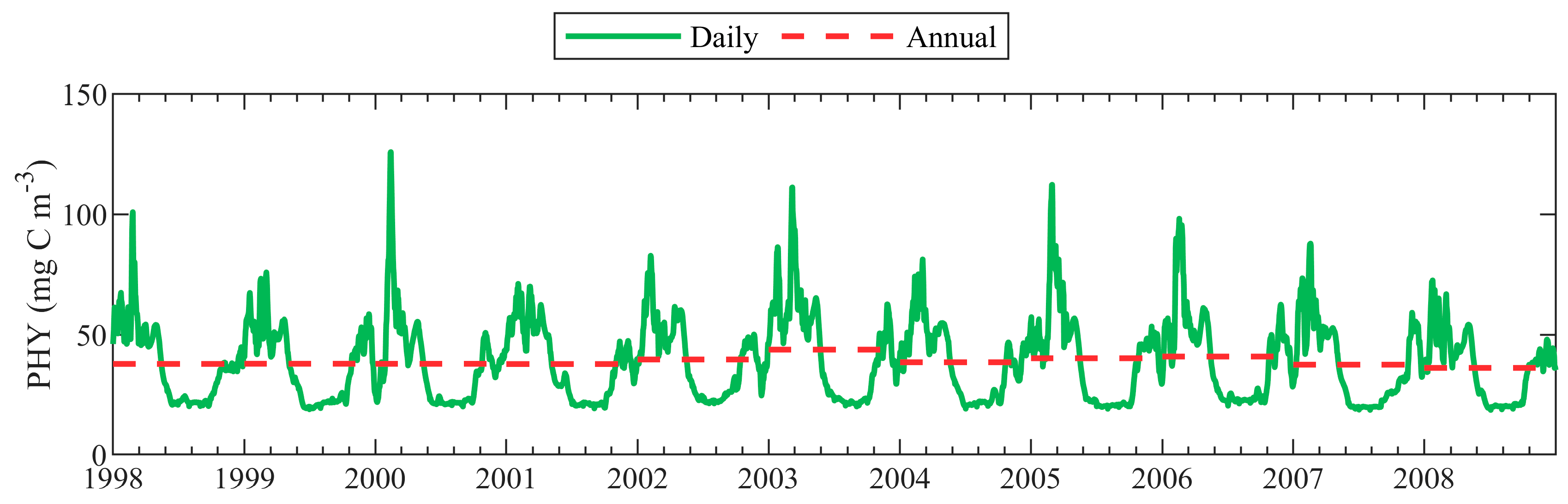
Given that this study aims to better describe the seasonal cycle and multi-annual variation of phytoplankton through the Black Sea, in Figure 7 are plotted the daily mean surface PHY (mg C m−3) model predictions, averaged over the whole deep basin (with depth > 1500 m). The annual mean surface PHY is shown with a dashed line. All annual mean values are close to the overall mean value (38.88 mg C m−3) for the whole simulation period. According to our bloom definition, the most abundant surface blooms take place in winter and early spring, while the surface bloom in summer is absent. The autumn bloom is clearly visible in our simulations, yet its amplitude is less than the corresponding winter bloom amplitude and of similar size to the spring bloom. Stronger winter blooms are calculated for the years with winter SST below the average.
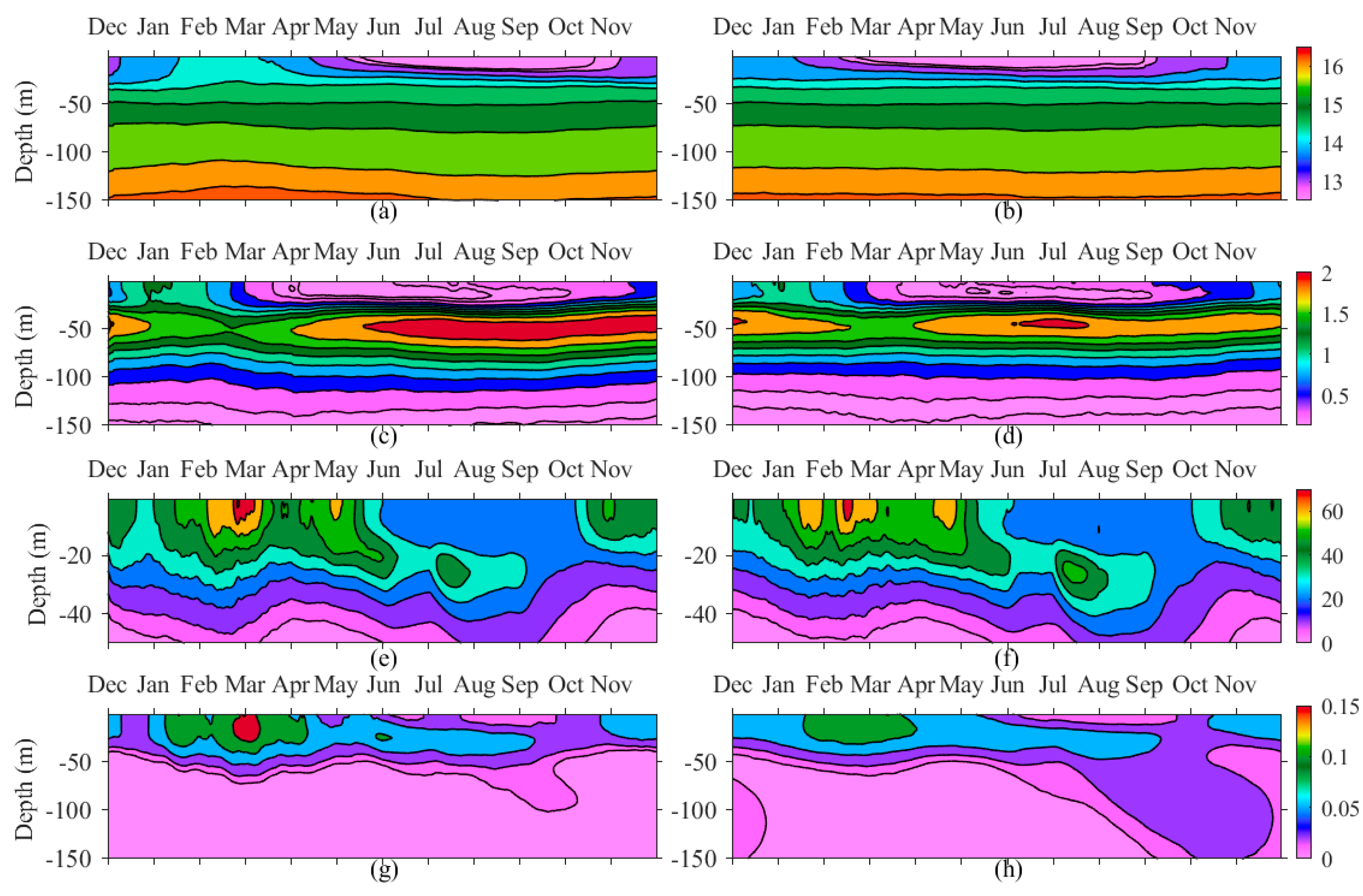
In Figure 8 are given climatological vertical distributions of (a–b) sigma density (kg m−3), (c–d) nitrate (mmol N m−3), (e–f) PHY (mg C m−3) and (g–h) detritus (mmol N m−3) averaged over the WEST region (Figure 1) from December to November in ‘cold’ and ‘warm’ years, as extracted from the BSEM output. First, we compute the seasonal cycle (365 days—each average of the 10-year period for ‘cold’ and ‘warm’ years, respectively). The seasonal cycle of the water column in the WEST region is then calculated by averaging the time series for all WEST model grid boxes. The WEST region is used as an example when comparing the mechanisms behind the blooms in both warm and cold periods. We find that the mechanisms governing blooms are closely related to the complexity of the physics in this deep-sea region. Note that the PHY profiles are plotted from the surface to 50 m depth, while the other variables are plotted down to 150 m depth. Typically, from mid-November to the end of February nitrate in the upper part of the storage (~60 m depth) rises and is utilised for biological production. Consistent with previous studies, simulations show that in ‘warm’ winters the entrainment of denser water into the mixed layer is lower (Figure 8a,b). During warmer winters, vertical surface mixing is reduced. The lower entrainment in warm winters results in a shallow winter mixed layer, which reduces the lift-up of nutrients from the pycnocline to the mixed layer (Figure 8c,d). Conversely, in ‘cold’ years, a stronger vertical mixing occurs in December through to February. Of note, in Figure 8c, the mechanism of the uplifting of nitrate from the storage and the increase of nitrate concentration in the mixed layer above 1 (mmol N m−3) can be seen.
The winter blooms in the WEST Black Sea region utilise the nitrate lifted from the storage and/or coming from the NWS. Generally, winter blooms start in January and attain maxima in February or the first half of March. The phytoplankton grows abundantly in the upper 15–25 m and decreases with depth (Figure 8e,f). A small amount of phytoplankton is mixed into the deeper water and is lost from the production regions of the water column. The BSEM model forecasts a winter bloom peak in January or February in ‘warm’ years and in February or March during ‘cold’ years. A lower phytoplankton bloom in December-January in the ‘cold’ years is compensated by higher bloom in the following two months (Figure 8e). The sunlight availability in December-January is an important factor in shaping the winter bloom. The winter surface cooling and strong winds that carry phytoplankton to depths below the euphotic zone have weaker negative effects on the phytoplankton abundance. Two distinct peaks (in January and February) are noticeable for the ‘warm’ years, followed by less pronounced blooms in March. Spring blooms are of smaller magnitude than the winter ones, and they attain a maximum in the second half of April for ‘warm’ years and at the end of April/beginning of May for ‘cold’ years. In summary, our results show, in agreement with the existing literature [5,55], that the lower winter nutrient supply from the storage in ‘warm’ years is a key factor in shaping the winter Black Sea phytoplankton bloom. In addition, our model clearly indicates the presence of both winter and spring blooms regardless of local meteorological and oceanographic conditions, and that the winter bloom in ‘cold’ years is more intense.
During summer months, DBM occurs in the thermocline at ~25–35 m depth and lasting June to September, fuelled by the nitrate in the storage. At the surface, PHY reaches a minimum in summer months. In the ‘warm’ summers, the DBM occurs in a slightly deeper location, and the PHY increases. An autumn bloom usually develops in October or November. Then, in December and in the first half of January, the bloom can decline, owing to low light intensity. The autumn peak occurs earlier and by the end of October in ‘cold’ years.
The detritus is mainly mineralised in the euphotic zone except for the amount produced by the summer phytoplankton growth in the thermocline (Figure 8g,h). The most obvious reason for detritus sinking in late summer is the lack of oxygen for mineralisation. The deep winter mixing causes deeper penetration of oxygen in the upper halocline, which can be used in late summer for detritus decomposition. For example, BSEM model simulations for the deep basin oxygen predict concentrations of over 50 (mmol O2 m−3) at about 100 m depth in the summers of 2003, 2006 and 2012 and close to zero in 2001 and 2011. The weaker winter, mixing in ‘warm’ years, results in a loss of subsurface organic matter in summer. At the end of February and beginning of March, the detritus in the upper 50 m reaches a maximum for ‘cold’ years. The nitrate storage is refilled to a greater extent in ‘cold’ years, which translates into a higher winter-spring detritus concentration.
4.2. Inter-Annual Variability of Plankton Blooms
Seasonality of the blooms is linked to the nitrate storage content, as well as to nutrient mixing during winter convection, as well as to the suppressed vertical mixing during the summer thermocline months. However, it is not fully understood how the nitrate storage is formed and how it correlates with the CIL dynamics. The CIL is defined in the literature as an intermediate layer with a temperature of less than 8 °C [56], while we assume it to be an intermediate layer, characterised by temperatures of less than 8.35 °C [35].
The Black Sea vertical thermohaline structure consists of a typical two-layer stratified system. The relatively low salinity surface water layer, which is approximately 100 m thick, is separated from the underlying water body by a permanent pycnocline located between sigma density σt ~ 14.5 and 16.5 kg m−3 (upper halocline). The strong vertical density gradients hinder the transport of nitrate from the halocline to the euphotic zone. Such transport of nitrate generally occurs in the deep basin by mechanisms of convection and advection in winter. The halocline acts not only as a barrier to vertical transport during these periods of thermocline presence, but it is also an essential nitrate source (Figure 8a–d).
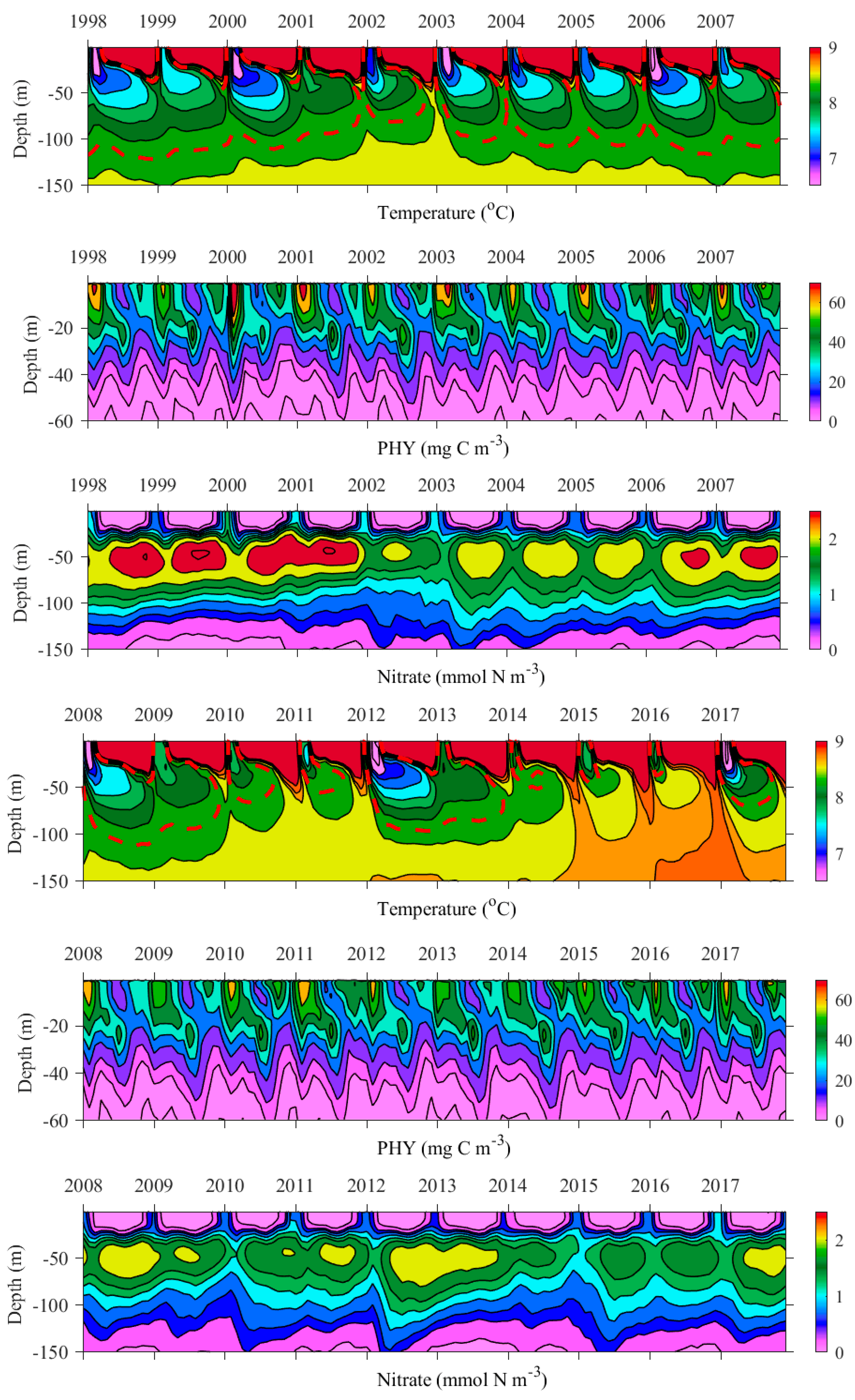
Figure 9 presents the vertical distribution of the inner basin mean temperature (°C), PHY (mmol C m−3) and nitrate (mmol N m−3) in the basin interior from the year 1998 to 2017. The vertical temperature profiles illustrate the CIL evolution in the inner basin (of depth > 1500 m) through the simulation period. From the model results, we can conclude that the storage is thicker and contains more nitrate when the CIL volume increases and its temperature decreases (Figure 9). That usually happens in ‘cold’ years, when the strong vertical winter mixing gives rise to strong phytoplankton growth in winter-spring, followed by the refilling of the nitrate storage with the regenerated nitrate. So, the CIL volume and temperature are important in regulating nitrate storage in the Black Sea waters. However, in several WARM years (e.g., 2010, 2011, 2015 and 2016) we found that the volume and/or nitrate content of the storage increase although the CIL is almost eroded. It is interesting to note that the storage has been substantially refilled in the years with high Danube discharge (e.g., 2010, 2015 and 2016). In 2010 the Danube discharge was extremely high, while 2015 and 2016 are the last two years of the four-year high Danube discharge period (discharges are significantly above the long-term mean levels). Thus, it turns out that both winter vertical mixing and Danube discharge are important for nitrate storage refilling.
Seasonal and inter-annual variation of the inner basin PHY is visible in Figure 9. The PHY reaches a maximum in winter with one exception in the year 2003 when it is shifted towards early spring. When comparing the winter-spring blooms in 1998–2009 and 2010–2017, there can be seen a tendency towards a smaller winter peak for the second period.
It is well known that the winter nitrate uplifting from the storage to the euphotic zone supports the winter-spring blooms. However, the storage in the years preceding the strong winter-spring blooms does not always contain high levels of nitrate (e.g., in 2002, 2015 and 2016). This is in accordance with [57], displaying that during severe winters, the content of nutrients in the CIL is not a reliable indicator of the bloom intensity. The convective mixing during the winter season is a dominant mechanism.
4.3. The Role of CIL
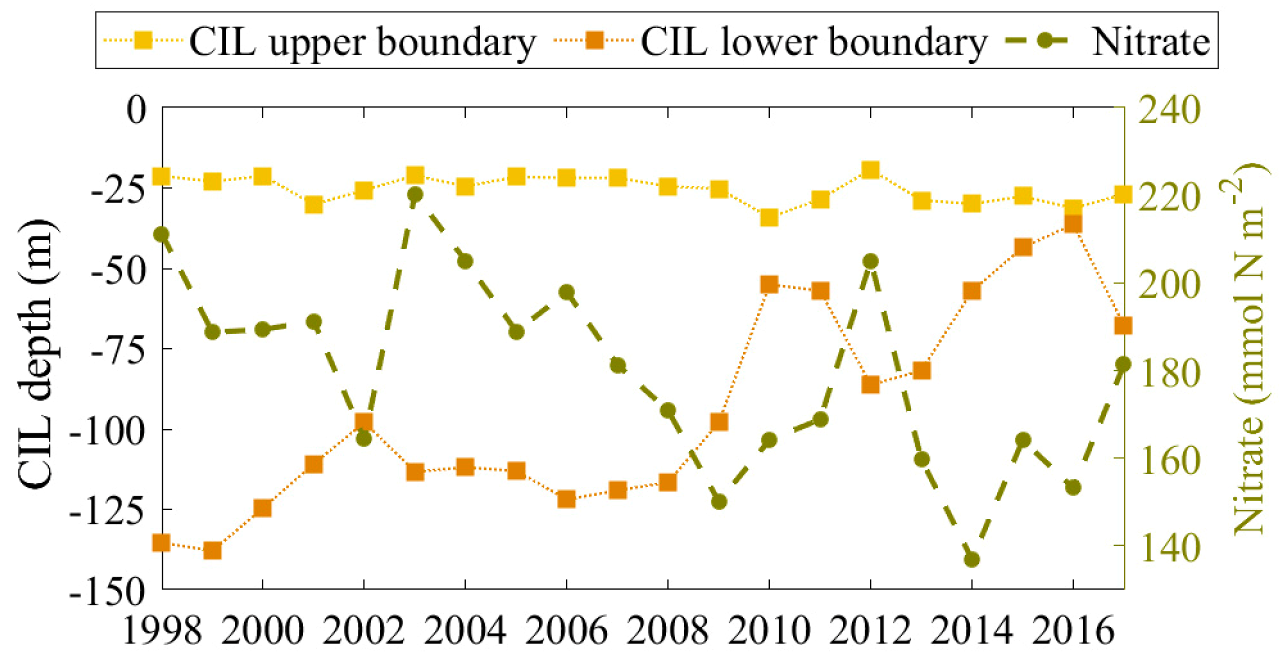
To study the impact of CIL evolution on nitrate content in the intermediate layers, the upper and lower CIL boundaries are presented together with the nitrate content in the pycnocline in Figure 10. The isotherm criteria for the CIL recognition (8.35 °C) is applied herein to identify its upper and lower boundary in the warm season. For example, the upper boundary is located at the first grid box below the surface where the temperature is lower than 8.35 °C. The lower boundary is located at the first grid box where the temperature becomes higher than 8.35 °C. Furthermore, CIL properties are averaged for the warm season (May-September) and over the deep basin (depth > 1500 m). During this season the CIL experiences less variation, due to a strong vertical stratification. Typically, the CIL upper boundary is about 25 m, however, it can be found exceeding 30 m depths in ‘warm’ years as a result of surface water warming. At the same time, the lower CIL boundary becomes shallower because of less intensive CIL refilling (see the red dashed line in Figure 9). In contrast, the depth of the CIL increases significantly in ‘cold’ years, mainly due to an intensified CIL refilling. The cold layer, defined as the water body having a temperature less than 8.35 °C, almost vanishes in 2016. The nitrate concentration in the storage is integrated along a vertical column, from 25 m depth (the upper boundary of the nitrate storage) to the seabed and then averaging is also performed across the entire warm months and over the entire extent of the deep basin. The annual nitrate variation simulated here is in accordance with the CIL variation (Table 3). For example, a significant positive correlation is found between the nitrate content and the upper/lower boundaries of CIL, while the correlation between nitrate content and CIL temperature is negative. Thus, the stronger the CIL, the higher the nitrate content of the pycnocline. Recently, the CIL is weak and eroded, and it is not surprising that the nitrate content of storage tends to decline (Figure 9).
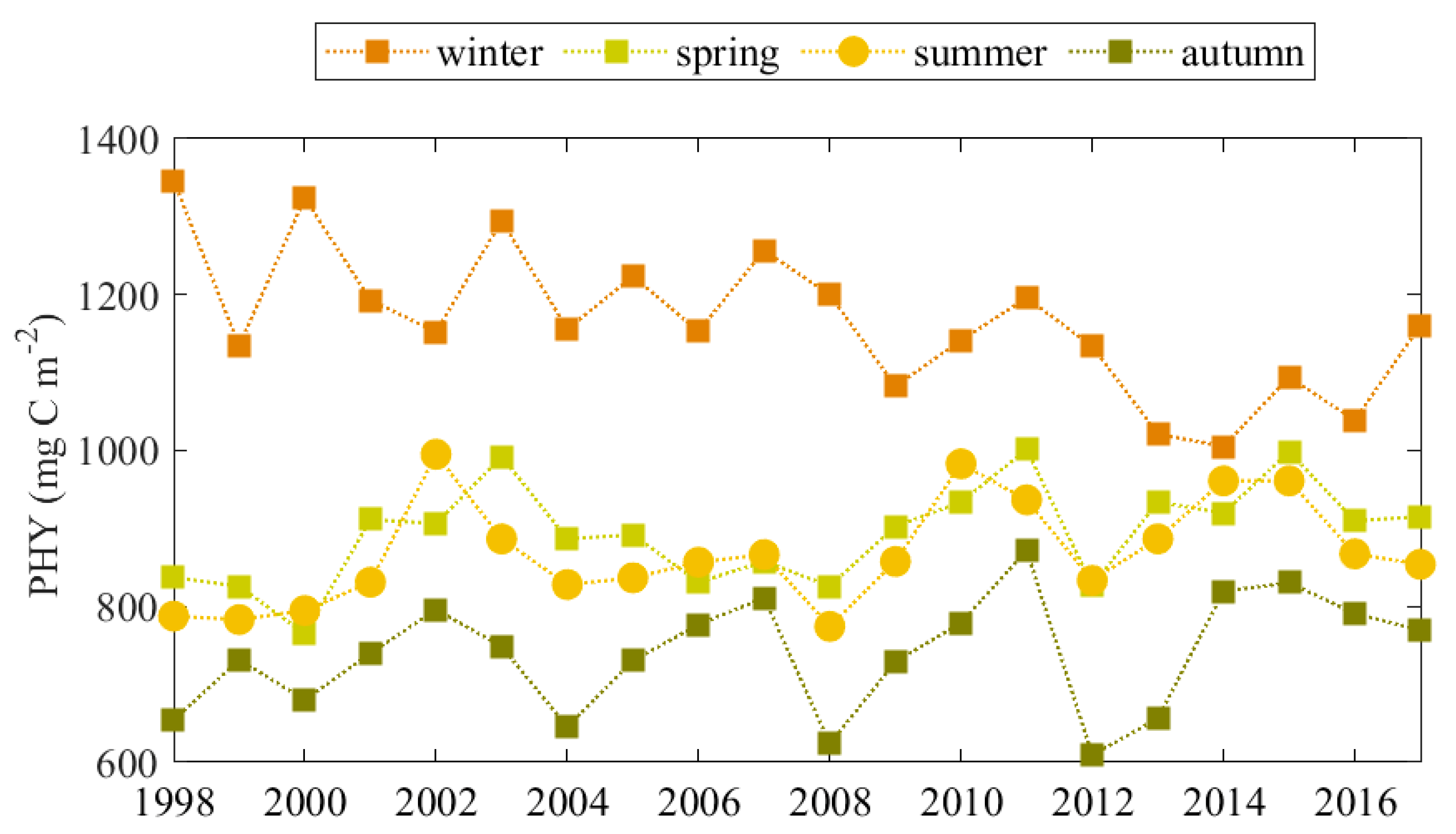
Winter, spring, summer and autumn PHY (mg C m−2) in the inner Black Sea basin are shown in Figure 11. They represent vertically integrated PHY values for the upper 50 m and are consequently averaged over the deep basin for January–March (winter PHY), April–May (spring PHY), June-September (summer PHY) and October–November (autumn PHY), respectively. Comparing the PHY successions in the deep Black Sea basin over the seasons, we highlight that the highest PHY is in the winter and is followed by the spring/summer PHY (both of similar magnitude). The seasonality found here agrees with previous studies [2,58]. The difference between the strength of winter and spring/summer PHY is reduced in recent years, for example, after 2009. The weakest value of PHY occurs in the autumn, however it increases in ‘warm’ years. A relationship between CIL properties and winter PHY is established. Like the nitrate content of pycnocline, the winter PHY is positively affected by the CIL strength (Table 3). The convective mixing during the winter season is a dominant mechanism for the CIL refilling, and essentially supports the nitrate lifting from the nitrate storage. On the contrary, the spring, summer and autumn PHY successions are favoured by the CIL weakness. A possible explanation includes an elevation of the CIL position toward the euphotic zone during periods of weak CIL. In this way, the nutrient storage is lifted-up, and the phytoplankton growth is enhanced. Note that autumn PHY does not correlate with nitrate content in the storage (Table 3), however the autumn PHY increases in periods of high Danube discharge. The factors influencing the increase of autumn PHY are presented and discussed in Section 4.4 and Section 4.5.
4.4. Mechanism behind Autumn Blooms in the Black Sea
The next topic of study is on the mechanisms behind the previously detected earlier autumn phytoplankton blooms. We found that the autumn surface bloom is always present it the Black Sea deep basin (Figure 7). The bloom usually begins in the second half of October (Figure 8c,d), when the PHY reaches values higher than 39 mg C m−3. However, in several years the phytoplankton blooms earlier in October (e.g., in 2011 among others, Figure 9). We set out to investigate the processes which are responsible for these premature blooms in autumn. Erosion of the thermocline and vertical mixing, due to surface cooling and strong winds typically start at the end of November, hence, they cannot be directly responsible for the early autumn bloom observed in References [9,55,59].
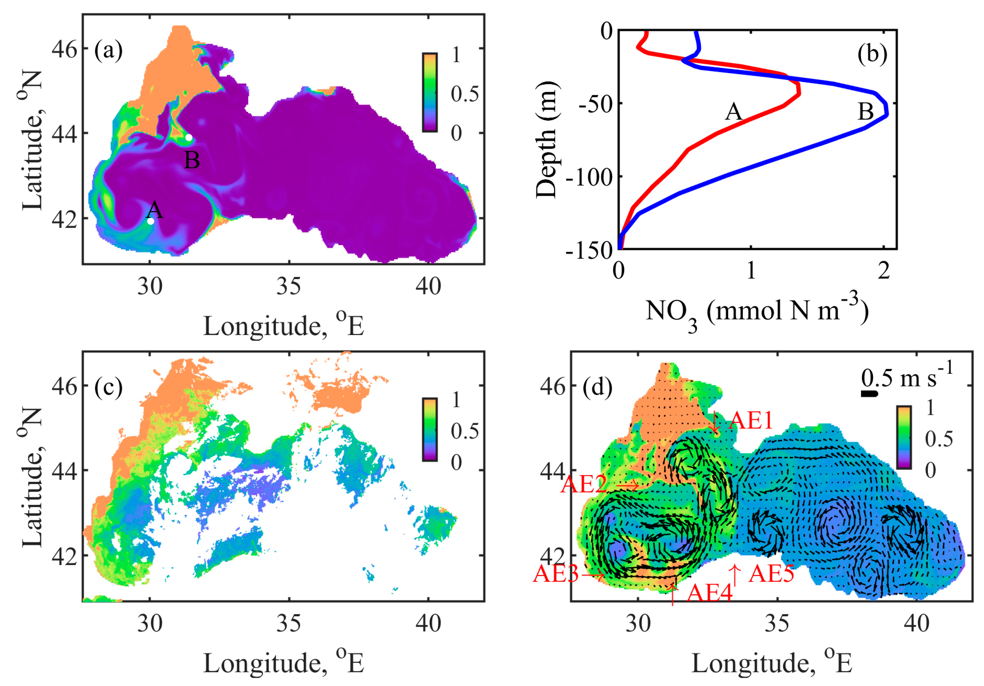
Figure 12 illustrates possible mechanisms for the early autumn bloom. We decided to illustrate the onset of bloom on 9 October 2004, due to the better quality of the satellite image on this day. The corresponding vertical profiles of nitrate in two specific geographic locations, indicated by A and B in Figure 12a, are plotted in Figure 12b. A daily nitrate distribution is included because nitrate is quickly utilised at the surface for biological production and disappears in days (Figure 12a). Figure 12c shows the SeaWiFS CHLa image, acquired on the same day [60], while the surface CHLa field and the surface currents, predicted by our modelling, are presented in Figure 12d. Previous modelling results [23,61] have shown that many MEs grow in late summer at spatial scales of 10–100 km and timescales of one month or more. The monthly velocity field given in Figure 12d could not capture all MEs which arose in a selected day. The western part of the Rim Current disintegrates into several vigorous cyclonic eddies.
On 9 October 2004, the Danube water transport is Northbound, then Eastbound and then flows offshore by the AE1 anticyclonic ME. Another part of the freshwater plume is partially locked by AE2 eddy, and then the plume splits toward west and east. The eastern part is mixed with the inner surface waters by the help of two energetic cyclonic eddies. One of them is located on the shelf-break, while another is in the inner basin. The western part of the plume moves along the west coast in a south-western direction. The spreading of the NWS waters towards the Anatolian coast is suppressed by AE3 eddy, which returns some of the water to the NWS circulation before reaching the Anatolian coast. At the Anatolian coast, the plume is transported to the western gyre by several anticyclonic MEs, two of them are AE4 and AE5. Then, the existence of cyclonic MEs inside the western gyre helps to further transport the bio-chemical matter (nitrate and biological material).
BSEM model results successfully reproduce the position and timing of the surface phytoplankton bloom caused by the NWS spreading (Figure 12c,d). SeaWiFS’s image contains many clouds, so the spread of CHLa from the south shelf-break into the inner basin is difficult to track. The NWS plume intrusion into the inner basin, induced by the MEs, can be seen to some extent in Figure 12c. In summary, the NWS waters were observed to mix laterally with the offshore waters through the shelf-break, due to the NWS anticyclonic eddies in our simulations. The cyclonic current of the west gyre transports nitrate and biological substances from the NWS to the southern part, where they are laterally mixed. Vertical nitrate profiles in Figure 12b show the existence of lateral surface mixing before the onset of vertical mixing. Cyclonic MEs in the inner basin contributes not only to the lateral mixing process, but also to the vertical uplift of nitrates to the surface.
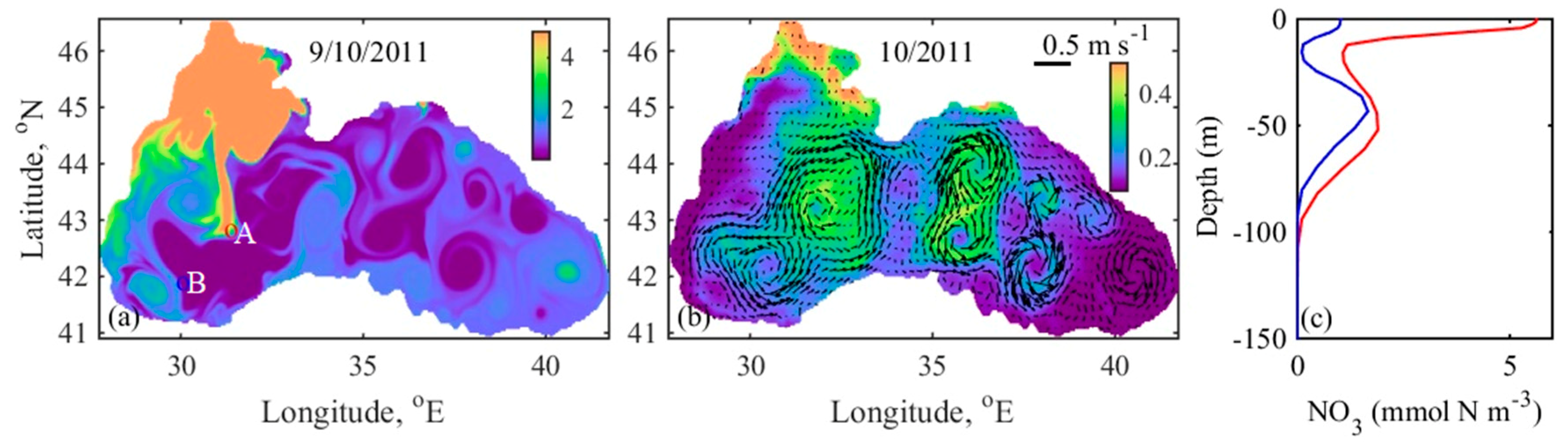
Another example of the onset of early autumn bloom is given in Figure 13. On 9 October 2011, the hydrodynamic conditions are more complicated, since the Danube waters are mainly carried to the north, partially move along the south coast and trapped offshore by the anticyclonic MEs. In the year 2004, the early October surface bloom decays in a week, and the next bloom starts in late November, after the onset of vertical mixing, due to surface cooling. In 2011, the penetration of fresher NWS water offshore and amplified mesoscale circulation triggered the vertical mixing and lift-up nitrate from the storage. Thus, blooming, beginning in the first half of October, lasts until late December (Figure 9). Penetration of the nitrate-rich peripheral water into the interior part of the sea, provoking one of the most abundant autumn blooms throughout the 20-year simulation period. A substantial infiltration of the peripheral water into the inner basin in autumn is associated with the typical late summer Rim Current disintegration (Figure 13b). In summary, the intensification of the autumn blooms can be attributed to a combination of several mechanisms–strengthening of the Rim Current in winter-spring prevents lateral mixing of NWS waters into the inner basin; intensification of the mesoscale and sub-mesoscale eddies in autumn provides favourable conditions for nutrient and biological substance transport from the periphery to the basin interior. The existence and timing of NWS break transport regarding plankton bloom dynamics of the Black Sea are discussed in the next and final subsection.
4.5. Mass and Volume Transport across the NWS Break
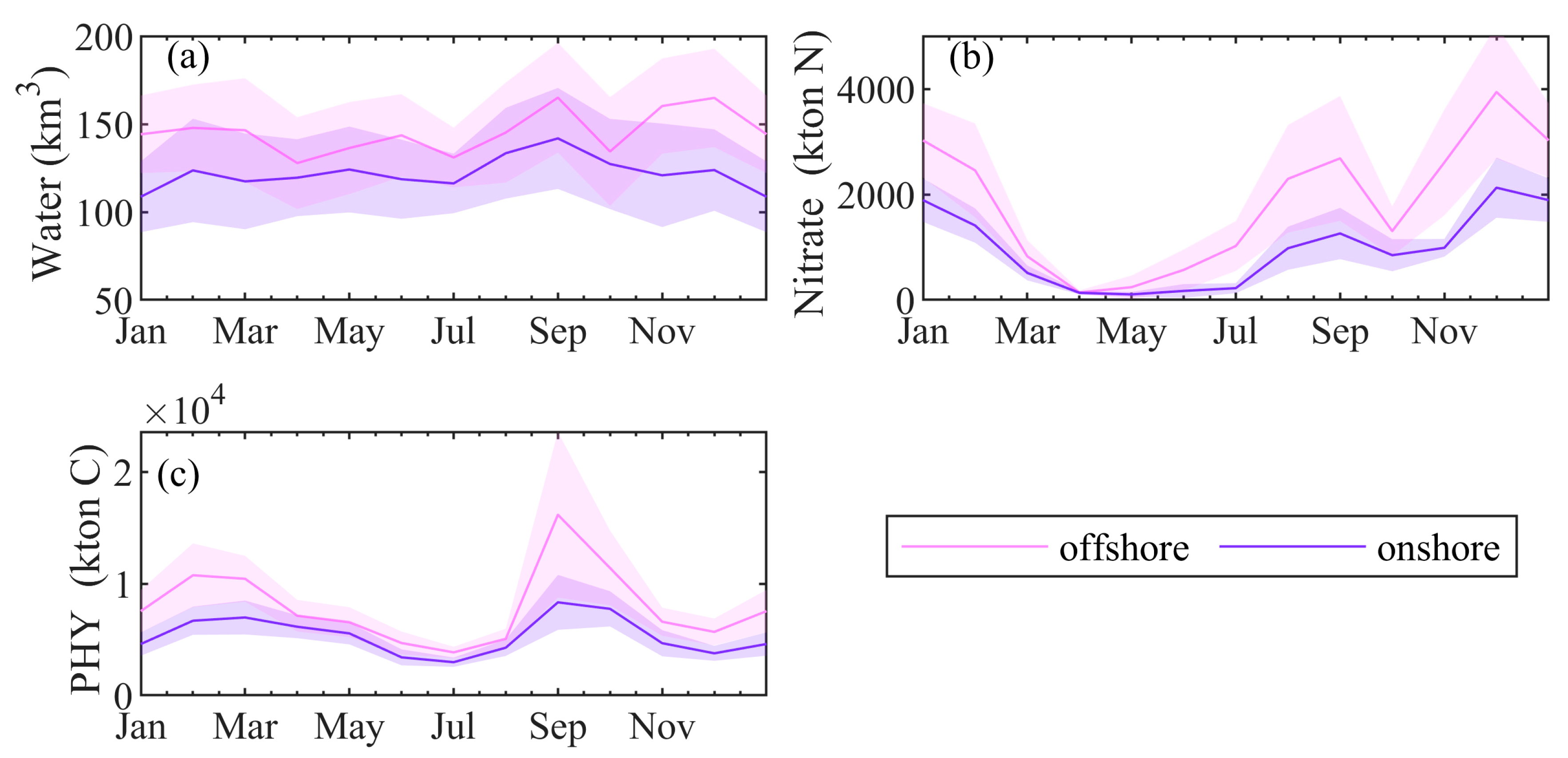
In Section 4.4, we showed that basin circulation supports lateral mixing in autumn. We will now provide supporting evidence for the strong influx of nitrate and biomass into the deep basin in September, which can fuel blooms of phytoplankton in October. Usually, the water masses coming from the NWS do not penetrate into the interior of the sea, where the salinity is higher, but are transported from the periphery of the Rim Current along the coast. A tendency of decreasing Danube plume transport, southward along the coastline and increasing transport to the north and north-eastern parts of the NWS and then to the southwest is established in Reference [61]. Moreover, it is shown that the river-borne substances achieve maximum concentrations in the inner basin in September. Following [62], we estimate the transport of water between the NWS and the Black Sea interior along with a boundary contouring the 200 m isobath, and including a segment connected to the coast of less than 20 m in depth (Figure 1, white path). For each day, the total transport is calculated by integrating the individual daily-averaged fluxes through the model grid boxes along the basin interior boundary in the horizontal plane and down to the 20 m layer in the vertical plane. The NWS freshwater plume usually forms a current, which is confined to the upper 25 m [63]. Offshore and onshore transports of nitrate and PHY through this boundary are also calculated. The water volume calculations across the NWS break show the presence of weak seasonal variation of the offshore/onshore transport (Figure 14a). Both offshore and onshore transports are plotted as positive values in Figure 14. The highest water volume, leaving and entering the NWS across the considered boundary occurs in September. We estimate that monthly offshore transport exceeds by about 20–30 km3 the onshore transport. Additionally, offshore and onshore transports display a similar seasonal variation.
Both offshore and onshore transport of nitrate (kton N) reach local maxima in September and then in December (Figure 14b), and minima in spring. A well-defined seasonal cycle is evident for the transport of nitrate and PHY (Figure 14b,c). The offshore nitrate transport is twice as large as the onshore transport. Interestingly, both nitrate transports are almost zero in April, indicating the depletion of nitrate in upper 20 m after the winter bloom.
The greatest seasonal fluctuations are predicted for the PHY (kton C) transport (Figure 14c). The maximum PHY transport occurs in September, prior to the autumn bloom, coinciding with the phytoplankton bloom on the NWS during this time. The smaller second peak of the PHY transport occurs in February and corresponds to the winter bloom on the NWS. Note that in September, the offshore PHY transport is over twice as the size of the onshore transport. The enhanced nitrate and PHY transport from the NWS to the inner basin in September can support early autumn blooms if the system circulation favours lateral transport.
5. Discussions and Conclusions
A modelling study of the phytoplankton evolution in the Black Sea inner basin during 1998–2017 is presented. The model is based on the coupling of GETM/GOTM and BSEM models. It reproduces the observed seasonal and annual growth of the phytoplankton adequately. An important factor influencing the discrepancy between the results of the BSEM model and the observed data is the conversion factor between N/C and CHLa. The C:CHLa ratio, within the mixed layer in the oligo/meso/eutrophic waters of the tropical Atlantic Ocean is estimated to be 145, 96 and 37, respectively [48]. Based on research conducted in the Black Sea from 2000 to 2011, the seasonal evolution of the C:CHLa ratio and its spatial variability in surface water layer (0–0.5 m) are analysed in Reference [64]. The maximum ratio is observed in summer months (~300 C:CHLa) and minimum value of ~50 in winter. Intermediate C:CHLa values are detected in spring and autumn. The main reasons for the temporal variability of the organic carbon to CHLa ratio are the variability in abundance of light, the seasonal variability in phytoplankton size, as well as in its taxonomic composition. To better compare the model (PHY) and the data (CHLa), an approach describing the dynamics of the C:CHLa ratio as a function of temperature, daily exposure and nutrient-restricted growth rate should be applied [49]. In its present configuration, the BSEM model simulates the phosphate limitation implicitly by linking it to nitrate dynamics using a fixed N:P ratio (Redfield). Future improvements of the model could include an explicit representation of the phosphate path through different state variables to adopt a flexible N:P ratio according to recent approaches [65,66]. More observational data of the river nutrient loads are required in order to better understand the observed CHLa dynamics in the Black Sea.
The simulations illustrate the remarkable complexity of the physical and biological mechanisms in the Black Sea, and at the same time, reveal some intriguing regularities. Despite its decreasing tendency, the winter phytoplankton bloom is still the most abundant seasonal bloom. Winter biomass production is closely related to the CIL dynamics and is essentially supported by the nitrate lifting from the storage in winter. Spring/summer blooms increase in ‘warm’ years, when the Danube discharge is high or when the CIL is weak. Both spring and summer blooms show an increasing tendency over the simulation period. Model results suggest that the timing of autumn phytoplankton bloom in the inner basin is related to high fluxes of nitrate and PHY across the NWS break in September. Mechanisms responsible for extensive autumn blooms include amplification of the Danube discharge, weakness of the CIL, and the abundance of energetic cyclonic and anticyclonic mesoscale eddies in late summer–autumn. Generally, they induce horizontal transport of nitrate and biological matter and generate autumn phytoplankton blooms, which consequently spread over the basin. Our future studies will address the relationship between physical structures of oceanic fronts and biological activity in order to quantify the role of eddies for biology.
Supplementary Materials
The following are available online at https://www.mdpi.com/2673-1924/1/4/18/s1, BSEM model equations; Table S1. Food preference coefficients of the predator groups on the prey groups; Table S2. BSEM input parameters.
Author Contributions
S.M.: Conceptualization, Methodology, Software, Writing—original draft. A.S.: Supervision, Project administration, Funding acquisition, Writing—review & editing. D.M.M.: Conceptualization, Methodology, Writing—review & editing. E.G.-G.: Data curation, Visualization, Software. All authors have read and agreed to the published version of the manuscript.
Funding
This research received no external funding.
Acknowledgments
We thank to “The Global Runoff Data Centre, 56068 Koblenz, Germany” for the Danube daily discharge rates. Special thanks go to the GETM/GOTM/FABM developers for providing and maintaining the model. Proofreading and fruitful discussions with Peter D. Marinov are gratefully acknowledged.
Conflicts of Interest
The authors declare no conflict of interest.
References
- Smayda, T.J. What is a bloom? A commentary. Limnol. Oceanogr. 1997, 42, 1132–1136. [Google Scholar] [CrossRef]
- Vedernikov, V.I.; Demidov, A.B. Vertical Distribution of Primary Production and Chlorophyll during Different Seasons in Deep Regions of the Black Sea. Oceanology 1997, 37, 376–384. [Google Scholar]
- Nezlin, N.P. Seasonal and interannual variability of remotely sensed chlorophyll. In The Handbook of Environmental Chemistry; Kostianoy, G., Kosarev, A.N., Eds.; Springer: Berlin/Heidelberg, Germany, 2006; pp. 333–349. [Google Scholar]
- Finenko, Z.Z.; Suslin, V.V.; Kovaleva, I.V. Seasonal and long-term dynamics of the chlorophyll concentration in the Black Sea according to satellite observations. Oceanology 2014, 54, 596–605. [Google Scholar] [CrossRef]
- Oguz, T.; Cokacar, T.; Malanotte-Rizzoli, P.; Ducklow, H.W. Climatic warming and accompanying changes in the ecological regime of the Black Sea during 1990s. Glob. Biogeochem. Cycles 2003, 17. [Google Scholar] [CrossRef] [Green Version]
- Oguz, T.; Dippner, J.W.; Kaymaz, Z. Climatic regulation of the Black Sea hydro-meteorological and ecological properties at interannual-to-decadal time scales. J. Mar. Syst. 2006, 60, 235–254. [Google Scholar] [CrossRef]
- Oguz, T. Long-Term Impacts of Anthropogenic Forcing on the Black Sea Ecosystem. Oceanography 2005, 18, 112–121. [Google Scholar] [CrossRef] [Green Version]
- McQuatters-Gollop, A.; Mee, L.D.; Raitsos, D.E.; Shapiro, G.I. Non-linearities, regime shifts and recovery: The recent influence of climate on Black Sea chlorophyll. J. Mar. Syst. 2008, 74, 649–658. [Google Scholar] [CrossRef] [Green Version]
- Mikaelyan, A.S.; Chasovnikov, V.K.; Kubryakov, A.A.; Stanichny, S.V. Phenology and drivers of the winter–spring phytoplankton bloom in the open Black Sea: The application of Sverdrup’s hypothesis and its refinements. Prog. Oceanogr. 2017, 151, 163–176. [Google Scholar] [CrossRef]
- Oguz, T.; Ediger, D. Comparision of in situ and satellite-derived chlorophyll pigment concentrations, and impact of phytoplankton bloom on the suboxic layer structure in the western Black Sea during May-June 2001. Deep. Res. Part II Top. Stud. Oceanogr. 2006, 53, 1923–1933. [Google Scholar] [CrossRef]
- BSC2008 State of Environment of the Black Sea (2001–2006/7). Available online: http://www.blacksea-commission.org/_publ-SOE2009.asp (accessed on 14 September 2020).
- Kubryakov, A.A.; Stanichny, S.V.; Zatsepin, A.G.; Kremenetskiy, V.V. Long-term variations of the Black Sea dynamics and their impact on the marine ecosystem. J. Mar. Syst. 2016, 163, 80–94. [Google Scholar] [CrossRef]
- Oguz, T.; Ducklow, H.; Malanotte-Rizzoli, P.; Tugrul, S.; Nezlin, N.P.; Unluata, U. Simulation of annual plankton productivity cycle in the Black Sea by a one-dimensional physical-biological model. J. Geophys. Res. Ocean. 1996, 101, 16585–16599. [Google Scholar] [CrossRef] [Green Version]
- Grégoire, M. Modeling the nitrogen cycling and plankton productivity in the Black Sea using a three-dimensional interdisciplinary model. J. Geophys. Res. Ocean. 2004, 109, C05007. [Google Scholar] [CrossRef] [Green Version]
- Oguz, T.; Salihoglu, B. Simulation of eddy-driven phytoplankton production in the Black Sea. Geophys. Res. Lett. 2000, 27, 2125–2128. [Google Scholar] [CrossRef]
- Tsiaras, K.P.; Kourafalou, V.H.; Davidov, A.; Staneva, J. A three-dimensional coupled model of the Western Black Sea plankton dynamics: Seasonal variability and comparison to Sea WiFS data. J. Geophys. Res. Ocean. 2008, 113. [Google Scholar] [CrossRef]
- Zatsepin, A.G. Observations of Black Sea mesoscale eddies and associated horizontal mixing. J. Geophys. Res. 2003, 108, 3246. [Google Scholar] [CrossRef]
- Kubryakov, A.A.; Bagaev, A.V.; Stanichny, S.V.; Belokopytov, V.N. Thermohaline structure, transport and evolution of the Black Sea eddies from hydrological and satellite data. Prog. Oceanogr. 2018, 167, 44–63. [Google Scholar] [CrossRef]
- Konovalov, S.K.; Murray, J.W. Variations in the chemistry of the Black Sea on a time scale of decades (1960–1995). J. Mar. Syst. 2001, 31, 217–243. [Google Scholar] [CrossRef]
- Oguz, T.; Velikova, V. Abrupt transition of the northwestern Black Sea shelf ecosystem from a eutrophic to an alternative pristine state. Mar. Ecol. Prog. Ser. 2010. [Google Scholar] [CrossRef]
- Kideys, A.E. ECOLOGY: Enhanced: Fall and Rise of the Black Sea Ecosystem. Science (80-) 2002, 297, 1482–1484. [Google Scholar] [CrossRef]
- Oguz, T.; Fach, B.; Salihoglu, B. Invasion dynamics of the alien ctenophore Mnemiopsis leidyi and its impact on anchovy collapse in the Black Sea. J. Plankton Res. 2008, 30, 1385–1397. [Google Scholar] [CrossRef]
- Miladinova, S.; Stips, A.; Garcia-Gorriz, E.; Macias Moy, D. Black Sea thermohaline properties: Long-term trends and variations. J. Geophys. Res. Ocean. 2017, 122, 5624–5644. [Google Scholar] [CrossRef] [PubMed]
- Ærtebjerg, G.; Carstensen, J. Indicator Fact Sheet: (WEU4) Nutrients in Coastal Waters. Available online: https://www.eea.europa.eu/data-and-maps/indicators/nutrients-in-coastal-waters-1/ (accessed on 14 September 2020).
- Tugrul, S.; Basturk, O.; Saydam, C.; Yilmaz, A. Changes in the hydrochemistry of the Black Sea inferred from water density profiles. Nature 1992, 359, 137–139. [Google Scholar] [CrossRef]
- Churilova, T.; Suslin, V.; Krivenko, O.; Efimova, T.; Moiseeva, N.; Mukhanov, V.; Smirnova, L. Light absorption by phytoplankton in the upper mixed layer of the Black Sea: Seasonality and parametrization. Front. Mar. Sci. 2017, 4, 1–14. [Google Scholar] [CrossRef] [Green Version]
- McCarthy, J.J.; Yilmaz, A.; Coban-Yildiz, Y.; Nevins, J.L. Nitrogen cycling in the offshore waters of the Black Sea. Estuar. Coast. Shelf Sci. 2007, 74, 493–514. [Google Scholar] [CrossRef]
- Yunev, O.A.; Carstensen, J.; Moncheva, S.; Khaliulin, A.; Aertebjerg, G.; Nixon, S. Nutrient and phytoplankton trends on the western Black Sea shelf in response to cultural eutrophication and climate changes. Estuar. Coast. Shelf Sci. 2007. [Google Scholar] [CrossRef]
- Oguz, T.; Latun, V.S.; Latif, M.A.; Vladimirov, V.V.; Sur, H.I.; Markov, A.A.; Özsoy, E.; Kotovshchikov, B.B.; Eremeev, V.V.; Ünlüata, Ü. Circulation in the surface and intermediate layers of the Black Sea. Deep. Res. Part I 1993, 40, 1597–1612. [Google Scholar] [CrossRef]
- Korotaev, G.; Oguz, T.; Nikiforov, A.; Koblinsky, C. Seasonal, interannual, and mesoscale variability of the Black Sea upper layer circulation derived from altimeter data. J. Geophys. Res. Ocean. 2003, 108. [Google Scholar] [CrossRef]
- GETM, 3D General Estuarine Transport Model. Available online: http://www.getm.eu/ (accessed on 1 October 2020).
- ECMWF, European Centre for Medium Range Weather Forecast. Available online: http://www.ecmwf.int (accessed on 10 October 2020).
- GRDC, Global Runoff Data Centre. Available online: http://www.bafg.de/GRDC (accessed on 10 October 2020).
- MEDAR/MEDATLAS II Project. Available online: http://www.ifremer.fr/medar (accessed on 10 October 2020).
- Miladinova, S.; Stips, A.; Garcia-Gorriz, E.; Macias Moy, D. Formation and changes of the Black Sea cold intermediate layer. Prog. Oceanogr. 2018, 167, 11–23. [Google Scholar] [CrossRef]
- Miladinova, S.; Stips, A.; Garcia-Gorriz, E.; Macias Moy, D. Modelling Toolbox 2: The Black Sea Ecosystem Model; Publications Office of the European Union: Luxemburg, 2016. [Google Scholar]
- Oguz, T.; Ducklow, H.W.; Malanotte-Rizzoli, P.; Murray, J.W.; Shushkina, E.A.; Vedernikov, V.I.; Unluata, U. A physical-biochemical model of plankton productivity and nitrogen cycling in the Black Sea. Deep Res. Part I Oceanogr. Res. Pap. 1999. [Google Scholar] [CrossRef]
- Oguz, T. Modeling aggregate dynamics of transparent exopolymer particles (TEP) and their interactions with a pelagic food web. Mar. Ecol. Prog. Ser. 2017, 582, 15–31. [Google Scholar] [CrossRef]
- Oguz, T.; Merico, A. Factors controlling the summer Emiliania huxleyi bloom in the Black Sea: A modeling study. J. Mar. Syst. 2006, 59, 173–188. [Google Scholar] [CrossRef]
- Miladinova, S.; Adolf, S.; Diego, M.M.; Elisa, G.G. Revised Black Sea Ecosystem Model; Publications Office of the European Union: Luxemburg, 2017. [Google Scholar]
- Ludwig, W.; Dumont, E.; Meybeck, M.; Heussner, S. River discharges of water and nutrients to the Mediterranean and Black Sea: Major drivers for ecosystem changes during past and future decades? Prog. Oceanogr. 2009, 80, 199–217. [Google Scholar] [CrossRef]
- Tuǧrul, S.; Murray, J.W.; Friederich, G.E.; Salihoǧlu, I. Spatial and temporal variability in the chemical properties of the oxic and suboxic layers of the black sea. J. Mar. Syst. 2014, 135, 29–43. [Google Scholar] [CrossRef]
- Codispoti, L.A.; Friederich, G.E.; Murray, J.W.; Sakamoto, C.M. Chemical variability in the Black Sea: Implications of continuous vertical profiles that penetrated the oxic/anoxic interface. Deep Res. Part A 1991, 38, S691–S710. [Google Scholar] [CrossRef]
- Baştürk, Ö.; Tuğrul, S.; Konovalov, S.; Salihoğlu, İ. Variations in the Vertical Structure of Water Chemistry within the Three Hydrodynamically Different Regions of the Black Sea. In Sensitivity to Change: Black Sea, Baltic Sea and North Sea; Springer: Dordrecht, The Netherlands, 1997; pp. 183–196. [Google Scholar]
- Koçak, M.; Mihalopoulos, N.; Tutsak, E.; Violaki, K.; Theodosi, C.; Zarmpas, P.; Kalegeri, P. Atmospheric deposition of macronutrients (dissolved inorganic nitrogen and phosphorous) onto the Black Sea and implications on marine productivity. J. Atmos. Sci. 2016, 73, 1727–1739. [Google Scholar] [CrossRef]
- Kubilay, N.; Yemenicioglu, S.; Saydam, A.C. Airborne material collections and their chemical composition over the Black Sea. Mar. Pollut. Bull. 1995, 30, 475–483. [Google Scholar] [CrossRef]
- Carstensen, J.; Klais, R.; Cloern, J.E. Phytoplankton blooms in estuarine and coastal waters: Seasonal patterns and key species. Estuar. Coast. Shelf Sci. 2015, 162, 98–109. [Google Scholar] [CrossRef] [Green Version]
- Finenko, Z.Z.; Hoepffner, N.; Williams, R.; Piontkovski, S.A. Phytoplankton carbon to chlorophyll a ratio: Response to light, temperature and nutrient limitation. Mar. Ecol. J. 2003, II, 40–64. [Google Scholar] [CrossRef] [Green Version]
- Cloern, J.E.; Grenz, C.; Vidergar-Lucas, L. An empirical model of the phytoplankton chlorophyll: Carbon ratio-the conversion factor between productivity and growth rate. Limnol. Oceanogr. 1995, 40, 1313–1321. [Google Scholar] [CrossRef] [Green Version]
- Karl, D.M.; Knauer, G.A. Microbial production and particle flux in the upper 350 m of the Black Sea. Deep. Res. Part A 1991, 38, S921–S942. [Google Scholar] [CrossRef]
- Kopelevich, O.V.; Sheberstov, S.V.; Yunev, O.; Basturk, O.; Finenko, Z.Z.; Nikonov, S.; Vedernikov, V.I. Surface chlorophyll in the Black Sea over 1978–1986 derived from satellite and in situ data. J. Mar. Syst. 2002, 36, 145–160. [Google Scholar] [CrossRef]
- Knorr 2001, NATO 2001 Black Sea Expedition. Available online: https://www.ocean.washington.edu/cruises/Knorr2001/ (accessed on 10 October 2020).
- Kaiser, D.; Konovalov, S.; Schulz-Bull, D.E.; Waniek, J.J. Organic matter along longitudinal and vertical gradients in the Black Sea. Deep Res. Part I Oceanogr. Res. Pap. 2017, 129, 22–31. [Google Scholar] [CrossRef]
- CMEMS, Copernicus Marine Environment Monitoring Service. Available online: https://marine.copernicus.eu/ (accessed on 10 October 2020).
- Mikaelyan, A.S.; Kubryakov, A.A.; Silkin, V.A.; Pautova, L.A.; Chasovnikov, V.K. Regional climate and patterns of phytoplankton annual succession in the open waters of the Black Sea. Deep Res. Part I Oceanogr. Res. Pap. 2018, 142, 44–57. [Google Scholar] [CrossRef]
- Filippov, D.M. Water Circulation and Structure of the Black Sea; Nauka: Moscow, Russia, 1968. [Google Scholar]
- Mikaelyan, A.S.; Zatsepin, A.G.; Chasovnikov, V.K. Long-term changes in nutrient supply of phytoplankton growth in the Black Sea. J. Mar. Syst. 2013, 117–118, 53–64. [Google Scholar] [CrossRef]
- Yunev, O.A.; Vedernikov, V.I.; Basturk, O.; Yilmaz, A.; Kideys, A.E.; Moncheva, S.; Konovalov, S.K. Long-term variations of surface chlorophyll a and primary production in the open Black Sea. Mar. Ecol. Prog. Ser. 2002, 230, 11–28. [Google Scholar] [CrossRef]
- Silkin, V.A.; Pautova, L.A.; Giordano, M.; Chasovnikov, V.K.; Vostokov, S.V.; Podymov, O.I.; Pakhomova, S.V.; Moskalenko, L.V. Drivers of phytoplankton blooms in the northeastern Black Sea. Mar. Pollut. Bull. 2019, 138, 274–284. [Google Scholar] [CrossRef]
- NASA Ocean Color. Available online: http://oceancolor.gsfc.nasa.gov/ (accessed on 10 October 2020).
- Miladinova, S.; Stips, A.; Macias Moy, D.; Garcia-Gorriz, E. Pathways and mixing of the north western river waters in the Black Sea. Estuar. Coast. Shelf Sci. 2020, 236, 106630. [Google Scholar] [CrossRef]
- Zhou, F.; Shapiro, G.; Wobus, F. Cross-shelf exchange in the northwestern Black Sea. J. Geophys. Res. Ocean. 2014, 119, 2143–2164. [Google Scholar] [CrossRef] [Green Version]
- Oguz, T.; Malanotte-Rizzoli, P.; Aubrey, D. Wind and thermohaline circulation of the Black Sea driven by yearly mean climatological forcing. J. Geophys. Res. 1995, 100, 6845. [Google Scholar] [CrossRef]
- Stelmakh, L.V.; Gorbunova, T.I. Carbon-to-chlorophyll-a ratio in the phytoplankton of the Black Sea surface layer: Variability and regulatory factors. Ecol. Montenegrina 2018, 17, 60–73. [Google Scholar] [CrossRef] [Green Version]
- Galbraith, E.D.; Martiny, A.C. A simple nutrient-dependence mechanism for predicting the stoichiometry of marine ecosystems. Proc. Natl. Acad. Sci. USA 2015, 112, 8199–8204. [Google Scholar] [CrossRef] [PubMed] [Green Version]
- Macias, D.; Huertas, I.E.; Garcia-Gorriz, E.; Stips, A. Non-Redfieldian dynamics driven by phytoplankton phosphate frugality explain nutrient and chlorophyll patterns in model simulations for the Mediterranean Sea. Prog. Oceanogr. 2019, 173, 37–50. [Google Scholar] [CrossRef] [PubMed]
Figure 1.
Bathymetry and location map of the Black Sea, North Western Shelf (NWS) and South Western Self (SWS) regions, and the main rivers. The 1500 m isobath is given in magenta and the 200 m isobath in cyan. The area between these two isobaths is considered herein as a shelf-break region. The boundaries of the three deep basin compartments ‘WEST’, ‘CENTRAL’ and ‘EAST’ are shown. The southernmost region, characterised by water depth inferior to 1500 m, is called the southern shelf. Symbols show the R/V Knorr and MSM33 routes and position of ARGO’s drift stations (Table 1). The NWS boundary, where the offshore/onshore exchanges are estimated, is denoted by a white tracer.

Figure 2.
Schematic representation of the Black Sea Ecosystem Model (BSEM) model structure that includes the basic omnivorous food web and its interactions with the gelatinous carnivore predators Mnemiopsis, Beroe Ovata and Noctiluca.
Figure 2.
Schematic representation of the Black Sea Ecosystem Model (BSEM) model structure that includes the basic omnivorous food web and its interactions with the gelatinous carnivore predators Mnemiopsis, Beroe Ovata and Noctiluca.

Figure 3.
A comparison of CHLa (mg CHLa m−3) profiles, acquired empirically by Knorr 2001 R/V (red symbols) and BSEM predictions (the lines represent modelled vertical profiles in the stations of Knorr 2001 R/V) in (a) WEST, (b) NWS-SB and (c) SWSB.
Figure 3.
A comparison of CHLa (mg CHLa m−3) profiles, acquired empirically by Knorr 2001 R/V (red symbols) and BSEM predictions (the lines represent modelled vertical profiles in the stations of Knorr 2001 R/V) in (a) WEST, (b) NWS-SB and (c) SWSB.

Figure 4.
Taylor diagram comparing modelled and in-situ CHLa (mg CHLa m−3). (a) vertical profiles acquired by Knorr 2001 R/V and BSEM model predictions for the stations distributed in the WEST, NWS-SB and SWSB and (b) surface CHLa acquired by MSM33 and BSEM predictions.
Figure 4.
Taylor diagram comparing modelled and in-situ CHLa (mg CHLa m−3). (a) vertical profiles acquired by Knorr 2001 R/V and BSEM model predictions for the stations distributed in the WEST, NWS-SB and SWSB and (b) surface CHLa acquired by MSM33 and BSEM predictions.

Figure 5.
A comparison between eight-day mean surface CHLa (mg CHLa m−3) measurements and model predictions, within the different regions: (a) WEST; (b) CENTRAL; and (c) EAST. Green lines represent surface CHLa from BSEM model, blue points–RegAlg and red squares–Copernicus. Time series are given for the area mean, averaged over a specified sub-region.

Figure 6.
Comparison of surface monthly CHLa concentrations determined by our proposed BSEM model and data gathered by ARGO floats. Model results are extracted at ARGO’s geographical location points (Figure 1).
Figure 6.
Comparison of surface monthly CHLa concentrations determined by our proposed BSEM model and data gathered by ARGO floats. Model results are extracted at ARGO’s geographical location points (Figure 1).

Figure 7.
Daily mean surface phytoplankton biomass (PHY) (mg C m−3) model prediction averaged over the whole deep basin (with depth > 1500 m). The annual mean surface PHY (mg C m−3) is shown with a dashed line.
Figure 7.
Daily mean surface phytoplankton biomass (PHY) (mg C m−3) model prediction averaged over the whole deep basin (with depth > 1500 m). The annual mean surface PHY (mg C m−3) is shown with a dashed line.

Figure 8.
Climatological daily mean vertical distribution in the WEST region for: (a) Sigma density (kg m−3) in ‘cold’ years and (b) in ‘warm’ years; (c) nitrate (mmol N m−3) in ‘cold’ years and (d) in ‘warm’ years; (e) PHY (mg C m−3) in ‘cold’ years and (f) in ‘warm’ years; and (g) detritus (mmol N m−3) in ‘cold’ years and (h) in ‘warm’ years.

Figure 9.
Deep basin monthly modelled vertical contours of temperature (°C), PHY (mg C m−3) and nitrate (mmol N m−3) from the years 1998 to 2017. To facilitate reading, the temperature colour bar is set in the range 6.5–9 °C and the 8.35 °C isotherm is shown with a red dashed line.
Figure 9.
Deep basin monthly modelled vertical contours of temperature (°C), PHY (mg C m−3) and nitrate (mmol N m−3) from the years 1998 to 2017. To facilitate reading, the temperature colour bar is set in the range 6.5–9 °C and the 8.35 °C isotherm is shown with a red dashed line.

Figure 10.
Mean cold intermediate layers (CIL) upper and lower boundary (m) in the deep Black Sea basin, averaged over the warm season (May-September) and vertically integrated nitrate concentration in the pycnocline (right axis, in units of mmol N m−2).
Figure 10.
Mean cold intermediate layers (CIL) upper and lower boundary (m) in the deep Black Sea basin, averaged over the warm season (May-September) and vertically integrated nitrate concentration in the pycnocline (right axis, in units of mmol N m−2).

Figure 11.
Vertically integrated modelled PHY (mg C m−2) in the inner Black Sea basin—average PHY for January–March (winter), April–May (spring), June–September (summer) and October–November (autumn).
Figure 11.
Vertically integrated modelled PHY (mg C m−2) in the inner Black Sea basin—average PHY for January–March (winter), April–May (spring), June–September (summer) and October–November (autumn).

Figure 12.
Daily mean simulation results on 9 October 2004 (a) surface nitrate (mmol N m−3); (b) vertical nitrate profiles at two points (locations are marked by ‘o’s in (a)): A (31.633° E, 42.667° N)—red line and B (31.467° E, 43.667° N)—blue line; (c) satellite image of CHLa (mg CHLa m−3) and (d) CHLa fields and currents, the colour bar represents the CHLa (mg CHLa m−3), the arrows show the speed (m s−1), and direction of the currents, where the length of the 0.5 m s−1 arrow is shown for scale, AE1–AE5 denote the locations of the calculated anticyclonic MEs. To facilitate reading, the nitrate colour bar is set in the range 0–1 mmol N m−3, while the CHLa colour bar is set in the range 0–1 mg CHLa m−3.

Figure 13.
(a) Daily mean surface nitrate field on 9 October 2011 (mmol N m−3); (b) monthly mean surface CHLa fields and currents averaged over upper 5 m in October 2011, the colour bar represents the CHLa (mg CHLa m−3), the arrows show the speed (m s−1), and direction of the currents, where the length of the 0.5 m s−1 arrow is shown for scale; (c) vertical nitrate profiles at the two points, shown in (a) A (red line) and B (blue line). To facilitate reading, the nitrate colour bar is set in the range 0–5 mmol N m−3, while the CHLa colour bar is set in the range 0–0.5 mg CHLa m−3.

Figure 14.
Calculated monthly transport across the NWS of (a) water volume (km3); (b) nitrate (kton N) and (c) PHY (kton C). Mean offshore transport is presented by a pink line, while mean onshore transport by a purple line. Shaded areas represent 95% confidence intervals of the mean.
Figure 14.
Calculated monthly transport across the NWS of (a) water volume (km3); (b) nitrate (kton N) and (c) PHY (kton C). Mean offshore transport is presented by a pink line, while mean onshore transport by a purple line. Shaded areas represent 95% confidence intervals of the mean.


Table 1.
The chlorophyll-a (CHLa) datasets names and coverage areas over space and time.
| Short Name | Type of Dataset | Resolution | Coverage | References |
|---|---|---|---|---|
| Copernicus | Satellite (Copernicus OCTAC) | 1 × 1 km, 1-day average | 1998–2017, Surface of the entire basin (a lot of missing data in December and January) | [54] |
| RegAlg | Satellite (SeaWiFS) | 4 × 4 km, daily | 1999–2008, Mean surface data for several particular regions | [4] |
| Knorr 2001 | In-situ | Stations | 23 May to 10 June 2001 Vertical profiles in WEST, SWSB (south-western shelf-break areas) and NWS | [52] |
| MSM33 | In-situ | Stations | 11 November to 2 December 2013 | [53] |
| ARGO1 | In-situ | Profiling float | 2014, Vertical profiles in WEST and CENTRAL 2015, in WEST | [54] |
| ARGO2 | In-situ | Profiling float | 1 January to 18 October 2014 Vertical profiles in SS | [54] |
| ARGO3 | In-situ | Profiling float | 2016, Vertical profiles in WEST and CENTRAL | [54] |
Table 2.
The average absolute error (AAE) (mg CHLa m−3) and R between pairs of different time series of eight-day mean surface CHLa over 1999–2008 in WEST, CENTRAL and EAST Black Sea regions (Figure 5). AAE error (mg CHLa m−3) and 95% confidence intervals (in parentheses), in the case when p-value < 0.05 are shown.
| Region | WEST | CENTRAL | EAST | |||
|---|---|---|---|---|---|---|
| Data sources | AAE (±error) | R (interval) | AAE (±error) | R (interval) | AAE (±error) | R (interval) |
| RegAlg Copernicus | 0.275 ± 0.014 | 0.08 (0.05, 0.11) | 0.267 ± 0.019 | - | 0.259 ±0.032 | - |
| RegAlg BSEM | 0.197 ± 0.009 | 0.44 (0.42, 0.47) | 0.158 ± 0.008 | 0.58 (0.56, 0.60) | 0.151 ± 0.008 | 0.56 (0.54, 0.59) |
| Copernicus BSEM | 0.229 ± 0.013 | 0.08 (0.05, 0.11) | 0.220 ± 0.017 | - | 0.234 ± 0.031 | - |
Table 3.
Correlation matrix over 1998–2017 between mean CIL properties, vertically integrated PHY (mg C m−2) and Nitrate (mmol N m−2) in the pycnocline. It includes the R-coefficient (p-value < 0.05 for all correlations) and the 95% confidence interval.
Table 3.
Correlation matrix over 1998–2017 between mean CIL properties, vertically integrated PHY (mg C m−2) and Nitrate (mmol N m−2) in the pycnocline. It includes the R-coefficient (p-value < 0.05 for all correlations) and the 95% confidence interval.
| Winter PHY | Spring PHY | Summer PHY | Autumn PHY | Nitrate in the Storage | |
|---|---|---|---|---|---|
| CIL properties | R (interval) | ||||
| Temperature | −0.59 (−0.82, −0.20) | 0.75 (0.45, 0.89) | 0.67 (0.33, 0.86) | 0.65 (0.07, 0.77) | −0.76 (−0.9, −0.48) |
| Lower boundary | 0.64 (0.28, 0.84) | −0.65 (−0.85, −0.29) | −0.69 (−0.87, −0.35) | −0.51 (−0.78, −0.09) | 0.65 (0.3, 0.85) |
| Nitrate in the storage | 0.72 (0.41, 0.88) | - | −0.54 (−0.79, −0.12) | - | 1 |
Publisher’s Note: MDPI stays neutral with regard to jurisdictional claims in published maps and institutional affiliations. |
© 2020 by the authors. Licensee MDPI, Basel, Switzerland. This article is an open access article distributed under the terms and conditions of the Creative Commons Attribution (CC BY) license (http://creativecommons.org/licenses/by/4.0/).
Share and Cite
MDPI and ACS Style
Miladinova, S.; Stips, A.; Macias Moy, D.; Garcia-Gorriz, E. Seasonal and Inter-Annual Variability of the Phytoplankton Dynamics in the Black Sea Inner Basin. Oceans 2020, 1, 251-273. https://0-doi-org.brum.beds.ac.uk/10.3390/oceans1040018
AMA Style
Miladinova S, Stips A, Macias Moy D, Garcia-Gorriz E. Seasonal and Inter-Annual Variability of the Phytoplankton Dynamics in the Black Sea Inner Basin. Oceans. 2020; 1(4):251-273. https://0-doi-org.brum.beds.ac.uk/10.3390/oceans1040018
Chicago/Turabian StyleMiladinova, Svetla, Adolf Stips, Diego Macias Moy, and Elisa Garcia-Gorriz. 2020. "Seasonal and Inter-Annual Variability of the Phytoplankton Dynamics in the Black Sea Inner Basin" Oceans 1, no. 4: 251-273. https://0-doi-org.brum.beds.ac.uk/10.3390/oceans1040018