Statistical Decomposition of the Recent Increase in the Intensity of Tropical Storms


1
Risk Management Solutions Ltd., Peninsular House, 30 Monument Street, London EC3R 8NB, UK
2
Bath, UK
*
Author to whom correspondence should be addressed.
Oceans 2020, 1(4), 311-325; https://0-doi-org.brum.beds.ac.uk/10.3390/oceans1040021
Submission received: 21 October 2020
/
Revised: 6 December 2020
/
Accepted: 7 December 2020
/
Published: 11 December 2020
(This article belongs to the Special Issue Tropical Cyclone Future Projections)
Abstract
:In a recent paper, Kossin et al. showed that during the period from 1979 to 2017, there was a statistically significant increase in the ratio of category 3–5 to category 1–5 tropical storm fixes in the ADT-HURSAT satellite dataset of tropical cyclone observations. The sign of this increase is consistent with previously developed theory and modelling results for how tropical cyclones may change due to climate change. However, without further analysis, it is difficult to understand what the implications of this increase might be for present day tropical cyclone risk. It is also difficult to understand how tropical cyclone risk models might be adjusted to reflect this increase, since this ratio is not typically directly represented in such models. Our goal is therefore to understand the drivers for this increase in terms of changes in the numbers of fixes of different categories of storms in different basins, which are quantities that are more directly related to tropical cyclone risk and risk modelling. We use both heuristic and quantitative methods. We find that the increase in the ratio is mainly driven by a decrease in the denominator (the number of category 1–5 fixes) and to a small extent by a slight increase in the numerator (the number of category 3–5 fixes). The decrease in the denominator is mostly driven by a statistically significant reduction in the number of category 1 fixes outside the North Atlantic. The slight increase in the numerator is mostly driven by a statistically significant increase in the number of category 3–4 fixes in the North Atlantic. Based on these results, we discuss different ways in which the increase in the ratio could be represented in risk models.
1. Introduction
The effects of climate change on temperature and sea-level are mostly well understood and readily quantified, albeit with uncertainty. The effects of climate change on other variables, however, are generally less well understood. In this article, we consider aspects of the possible effects of climate change on the frequency and intensity of tropical cyclones, with a particular focus on quantities that are directly of relevance to tropical cyclone risk and risk modelling. There are essentially three methodologies that one can use to investigate the question of how the frequency and intensity of tropical cyclones might change. One is theory. There is no complete theory of tropical cyclones that can give good explanations for all the aspects of tropical cyclone behavior that are seen in nature. However, for the intensity of tropical cyclones, there is a body of theory [1] that can be used to attempt to predict how tropical cyclones might change in the future: the implications of this theory are that the intensities of individual tropical cyclones may have already increased, and may continue to increase, all other things being equal [2]. The second methodology that one can use to understand the possible effects of climate change on tropical cyclones is dynamical modelling of the climate using climate models. In a recent survey of climate model results for tropical cyclones [3], different models were found to give somewhat different results, highlighting the uncertainty, but many models showed decreasing overall frequency of tropical cyclones, the highest resolution models suggested an increase in the frequency of very intense tropical cyclones (strength categories 4 and 5), and most models showed an increase in the proportion of tropical cyclones that reach very intense. The third methodology that one can use to understand how tropical cyclones may change under a changing climate is to look at the past, and use statistical analysis to assess whether it is already possible to see any changes in tropical cyclone behavior that could be due to climate change. This is difficult for three particular reasons: tropical cyclones, especially the most intense tropical cyclones, are rare; past measurements of tropical cyclone behavior are inhomogeneous in coverage and quality [4]; and tropical cyclone behavior is affected by climate variability on multiple time-scales, much of which is not fully understood, and which hinders the detection of long-term trends [5]. As a result, there is no clear consensus, at this point, as to whether the impacts of climate change can be said to have been clearly detected in the historical record for tropical cyclones, although some claims have been made with respect to the increasing intensity of the strongest storms [6,7].
In a recent paper, Kossin et al. [8] described an analysis based on the latest version of the ADT-HURSAT dataset [9,10] (where ADT stands for Advanced Dvorak Technique and HURSAT stands for HURricane SATellite), in which they showed that there is a statistically significant (outside a 2.5%–97.5% confidence interval—henceforth “significant”) increase in the ratio of the number of category 3, 4 and 5 (cat35) fixes to the number of category 1, 2, 3, 4 and 5 (cat15) fixes in that dataset, over the period 1979 to 2017. Kossin et al. [8] used ADT-HURSAT, which is an objectively processed satellite dataset of global tropical cyclone observations, as it provides a more homogeneous time-series of tropical cyclone observations than the International Best Track Archive [11], even though the latter dataset may be more accurate in some ways. The fixes that they considered are 6 hourly measurements, and there are typically multiple fixes for each tropical storm. In general, cat35 fixes are defined as those that record windspeeds of 96+ knots, and cat15 fixes are those that record windspeeds of 64+ knots. Since in the ADT-HURSAT data intensity is discretized into 5 knot bins, this corresponds to windspeeds of 100+ knots and 65+ knots, respectively, in this dataset.
Kossin et al. [8] used a number of different statistical methods for investigating possible changes in the ratio of cat35 (henceforth major hurricane (MH)) to cat15 fixes (henceforth just “the MH ratio”), including consideration of the differences in the ratio between block averages of early and later periods of the data, and a linear trend analysis of the MH ratio combined into three-year sub-periods. These two methods both show significant signals corresponding to an increase in the MH ratio. They noted that this increase is consistent with theoretical and dynamical modelling results, which suggests an increase in the proportion of major tropical cyclones due to climate change [3].
However, from the point of view of tropical cyclone risk and risk modelling, the implications of this increase are hard to understand. The ratio of cat35 to cat15 fixes is not something that is explicitly included in most tropical cyclone risk models. In this article, our goal is therefore to analyze the increase identified in Kossin et al. [8] and understand what changes within the dataset are driving it, in terms of quantities that are more closely aligned with risk modelling. In particular, we will attempt to answer the following questions:
- (a)
- is the increase in the MH ratio driven by changes in the numerator (the number of cat35 fixes), the denominator (the number of cat15 fixes), or both?
- (b)
- is the increase in the MH ratio driven by any particular strength categories, or is it driven by several strength categories?
- (c)
- is the increase driven by any particular regions, or is it the result of similar changes in all regions?
These are arithmetical questions about the increase in the MH ratio, rather than being questions about the physical drivers or mechanisms behind the increase. Answers to these questions can help risk modelers decide how they could adjust risk models to reflect the increasing MH ratio, should they wish to.
In Section 2 below, we provide a brief review of the linear trend analysis that Kossin et al. [8] used to identify the increase. In Section 3, we provide a heuristic analysis to understand what might be driving the linear trend. In Section 4, we provide a quantitative analysis using decomposition of the trend slope to identify the statistical drivers behind the linear trend. In Section 5, we summarize and draw some conclusions.
2. Dataset and Increase in the MH Ratio
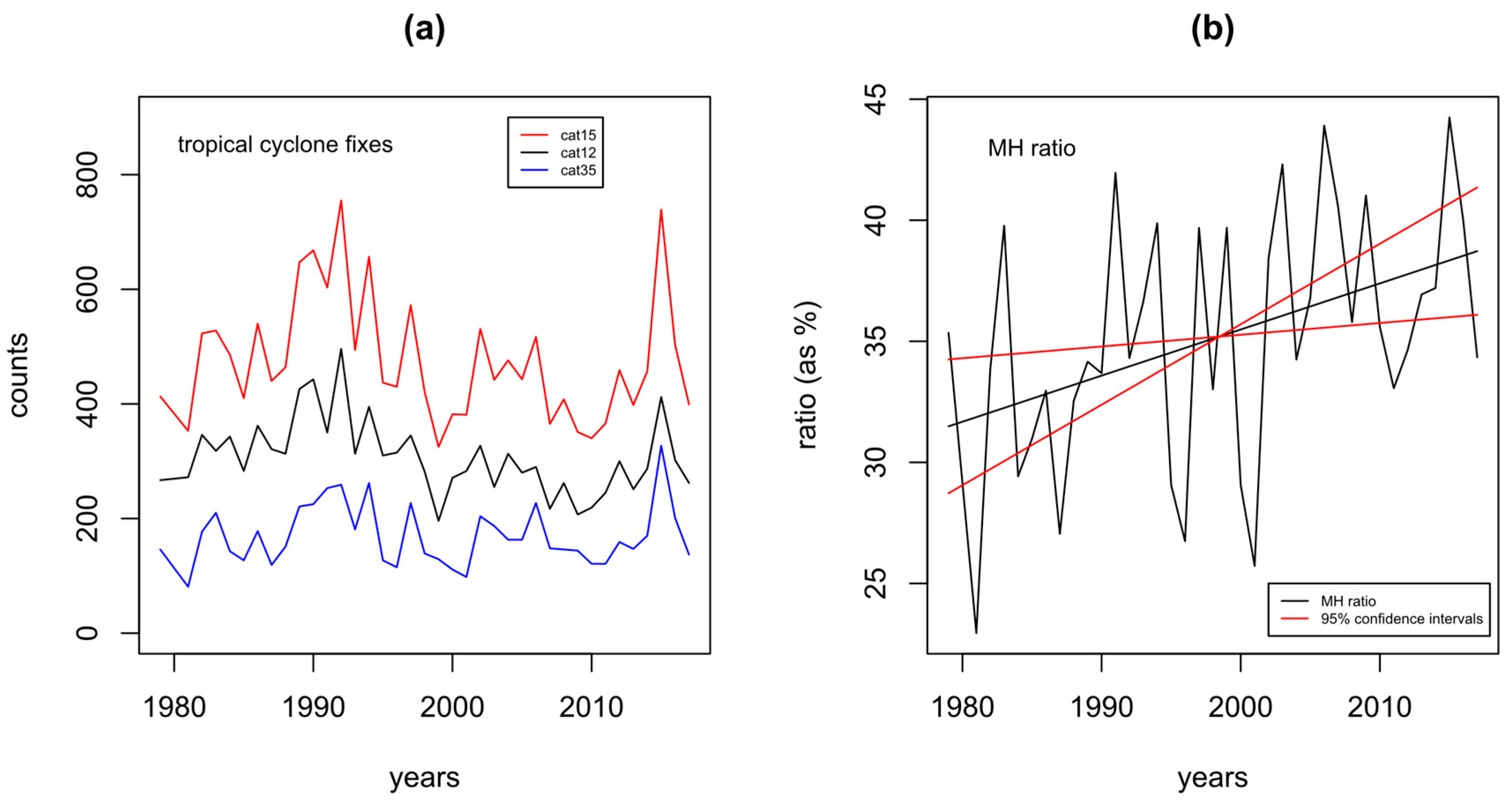
In this section, we briefly review the increase in the ADT-HURSAT MH ratio that was identified in Kossin et al. [8]. The ADT-HURSAT data we use for our analysis are available on the internet as part of the supplementary information provided by Kossin et al. [8]. Figure 1a shows the annual numbers of category 1 and 2 (cat12), cat35, and cat15 fixes in the ADT-HURSAT dataset, for the period 1979 to 2017. In this and all the subsequent analysis, we omitted 1980 for reasons of incomplete data, following Kossin et al. [8]. In all the time series plots, linear interpolation was used between 1979 and 1981, although the calculation of trend-lines and significance levels all treat 1980 as a missing value. We see from Figure 1a that the three time series are correlated. That cat15 is correlated with both cat12 and cat35 is not surprising since the cat15 numbers are simply the sum of the cat12 and cat35 numbers. That cat12 and cat35 are correlated is also not surprising, since each storm that reaches cat35 must pass through cat12. We also see that the vertical distance between the cat12 and cat35 time series tends to decrease over time and is lower in the second half of the series than the first.
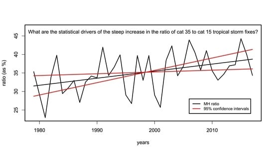
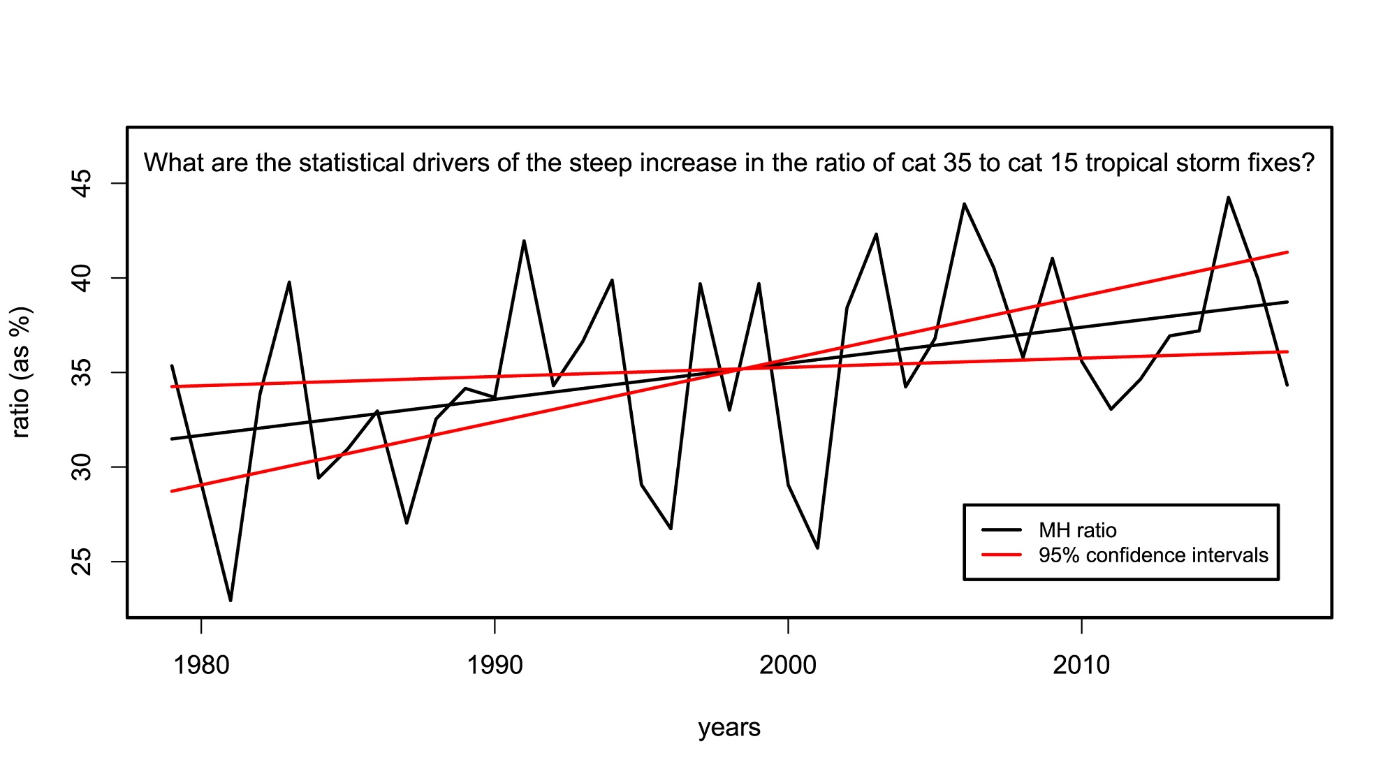
Figure 1b shows the MH ratio. When the MH ratio is created, much of the variability cancels out between the two datasets because of the correlation between the series. Kossin et al. [8] also argued that this cancellation includes some cancellation of observational errors. An example would be that if a cat35 storm is missed (e.g., due to satellite failure), it will be missed from both the cat35 and cat12 records and hence will have a minimal impact on the MH ratio. This cancellation of errors is one of the reasons why Kossin et al. [8] chose to focus on the ratio of cat35 to cat15 fixes, rather than the numbers of fixes themselves.
However, from the point of view of trying to inform tropical storm risk quantification, it is necessary to consider the data for the actual counts of fixes, not just the MH ratio, and that is what we will do below. Using counts means that our analysis is exposed to a greater extent to the impacts of observational errors and variability in the data, because we lose the advantage of the cancellation of errors mentioned above. This should be taken into account in the interpretation of the results below: the count data should not be used for quantifying subtle signals. However, the main drivers we identify in our analysis below will turn out to be large signals that are hopefully reasonably robust.
If we write as the number of cat12 fixes, as the number of cat35 fixes, and as the number of cat15 fixes then and the MH ratio is given by
That the cat12 and cat35 time series get closer together over time in Figure 1a implies that is reducing, which in turn implies that is increasing, which is what we see in Figure 1b.
One of the methods used by Kossin et al. [8] was to group the annual values of the MH ratio into triads (groups of three years), and consider statistical significance of a trend in the triad values, where the trend was fitted using Theil–Sen regression. As an alternative, and somewhat more simply, we fit a linear trend directly to the annual values shown in Figure 1b using ordinary least squares (OLS), with 1980 omitted. Using OLS facilitates the decomposition analysis we describe in Section 4 below. The OLS trend is also shown in Figure 1b. Above and below the OLS trend-line, we show two other lines which have the same mean as the OLS trend-line, but slopes which give the 95% confidence intervals around the trend slope. The OLS trend is positive and significant, with a p-value of p = 0.01.
Fitting a linear trend to these ratios is not strictly defensible, since the ratios are bounded between zero and one, while the trend line ultimately stretches from minus infinity to infinity. We tested the importance of avoiding this problem by transforming the ratios using a probit transform, to give them a possible range from minus infinity to plus infinity, before fitting the trend. This, however, made little difference to the results, since the range of the ratios is rather small, and the probit transform is close to linear over this range. For the remainder of our analysis, we proceed with the untransformed values for simplicity.
Based on Kossin et al.’s [8] analysis, and the linear trend analysis given above, there seems little doubt that the increase in the MH ratio is robust (i.e., is not an artefact of interannual variability in the dataset). However, from the point of view of fully understanding the implications of the increase for risk analysis, the question remains as to what is driving the increase.
3. Results
In this section, we perform a heuristic investigation to try to understand what might be driving the trend in the MH ratio. We will then complement this with a quantitative analysis in Section 4.
3.1. Numerator vs. Denominator
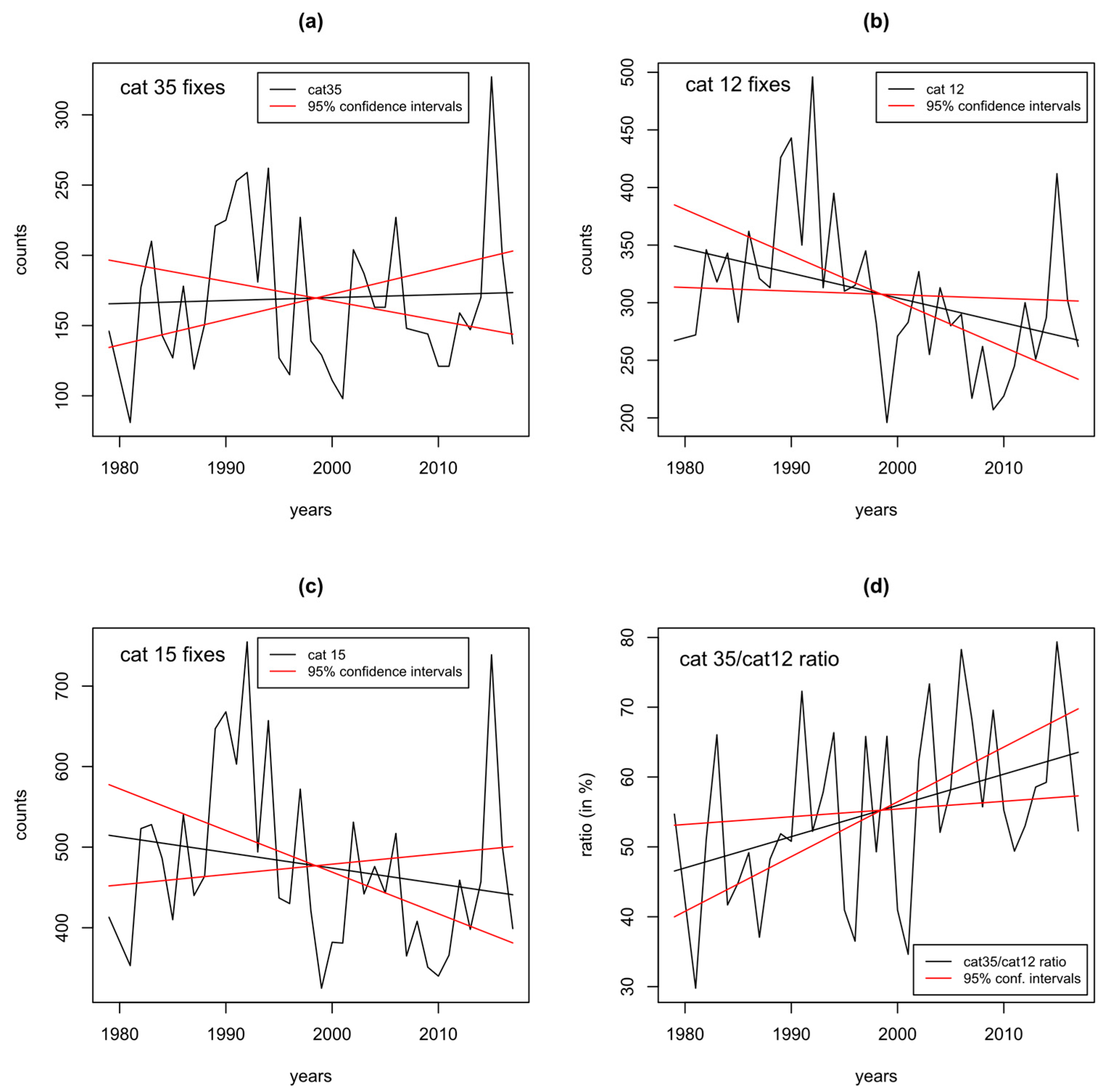
A first question one might ask about the cause of the trend shown in Figure 1b is: is it changes in the numerator of the ratio driving the trend, or the denominator of the ratio, or both? Figure 2a–c show the time series for the numerator (cat35 fixes), for cat12 fixes, and for the denominator (cat15 fixes), respectively, with linear trends fitted to all. The cat35 fixes show a very slight and not significant upward trend (p-value 0.79). The cat12 fixes show a significant downward trend (p-value 0.02). The cat15 fixes show a slight and not significant downward trend (p-value 0.23). Figure 2d shows the ratio of cat35 fixes to cat12 fixes, with a fitted trend, which has a positive slope. This is significant, with a p-value of 0.01. Table 1 summarizes the values of the significance levels of the main global trends in numbers of fixes for different strength categories.
Subject to quantitative confirmation in Section 4 below, we conclude from this that the upward trend in the MH ratio is to a small extent due to a non-significant upward trend in the cat35 fixes, but is mostly due to a downward trend in the cat15 fixes, which in turn is due to a significant downward trend in the cat12 fixes. Aspects of this downtrend were discussed in Holland and Bruyere [12].
3.2. Category of Storm Fixes
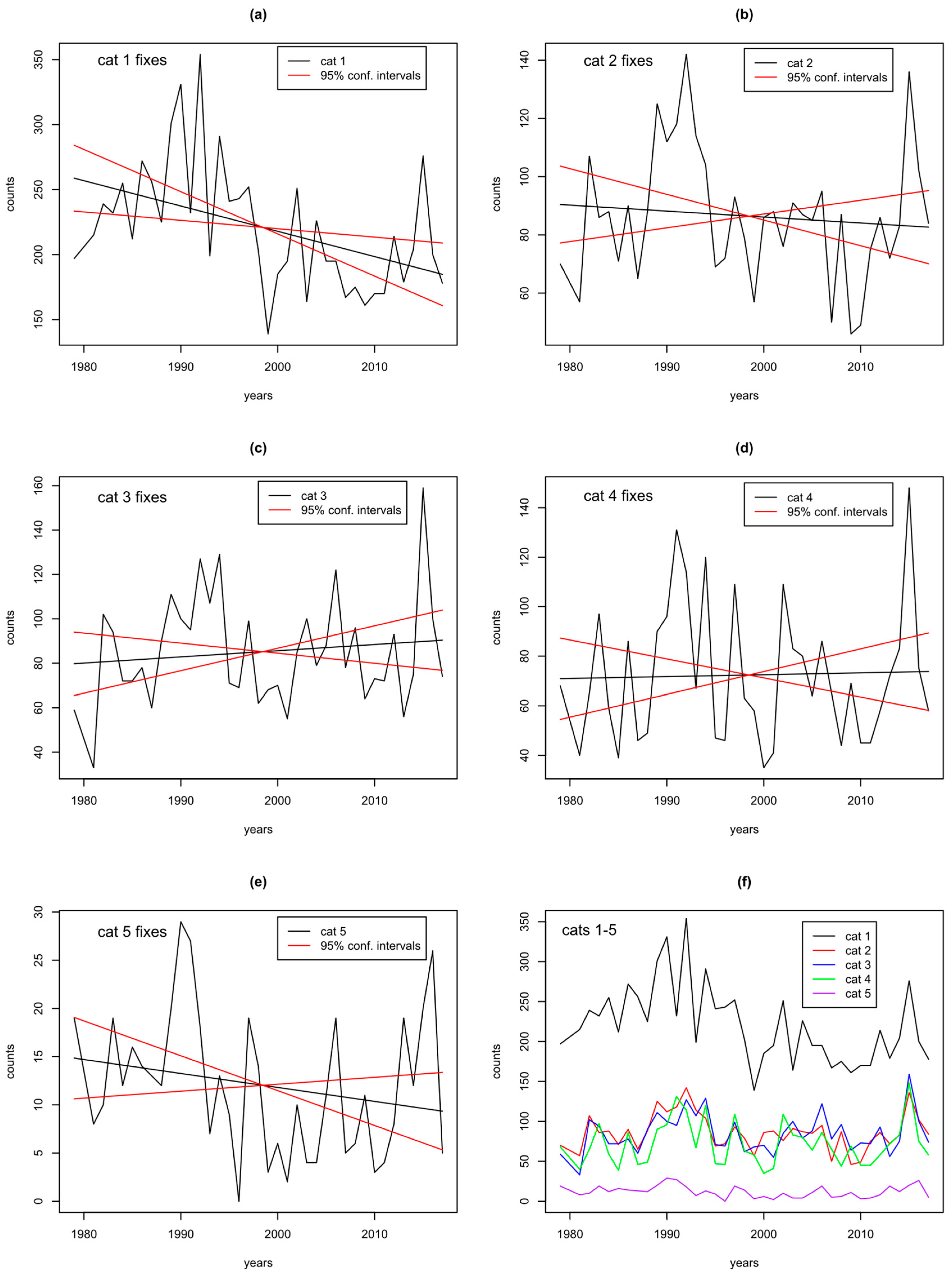
Given the above results, one might ask whether the upward trend in the cat35 fixes is due to cat3s, or cat4s, or cat5s, and whether the downward trend in cat12 fixes is due to cat1s or cat2s. Figure 3 shows trends for all five categories individually in sections (a) to (e). Trend slopes and p-values for the trends are given in Table 1. There is a strong and highly significant downward trend in the cat1 fixes (p-value 0.004), and a weak and not significant downward trend in the cat2 fixes. These two combine to give the downward trend in the cat12 fixes.
There are weak upward trends in the cat3 and cat4 fixes, and a downward trend in the cat5 fixes. None are significant but they combine to give the weak upward trend in the cat35 fixes. In the cat15 time series, the downward trend in cat12s is large enough to dominate the upward trend in the cat35s, to give a net downward trend overall. Combining this with the previous analysis leads us to conclude that the upward trend in the MH ratio is likely mostly driven by the significant downward trend in the cat1s.
3.3. Regional Analysis
Based on the above analysis, one might also ask which regions are driving the changes in cat1 and cat34 fixes. The ADT-HURSAT data categorize each storm into one of seven regions: North Atlantic (NA), Eastern North Pacific (EP), Western North Pacific (WP), South Pacific (SP), Southern Indian Ocean (SI), Northern Indian Ocean (NI), and South Atlantic (SA). The South Atlantic region, however, only has one storm with cat15 fixes and so we will ignore it and only consider the other six regions.
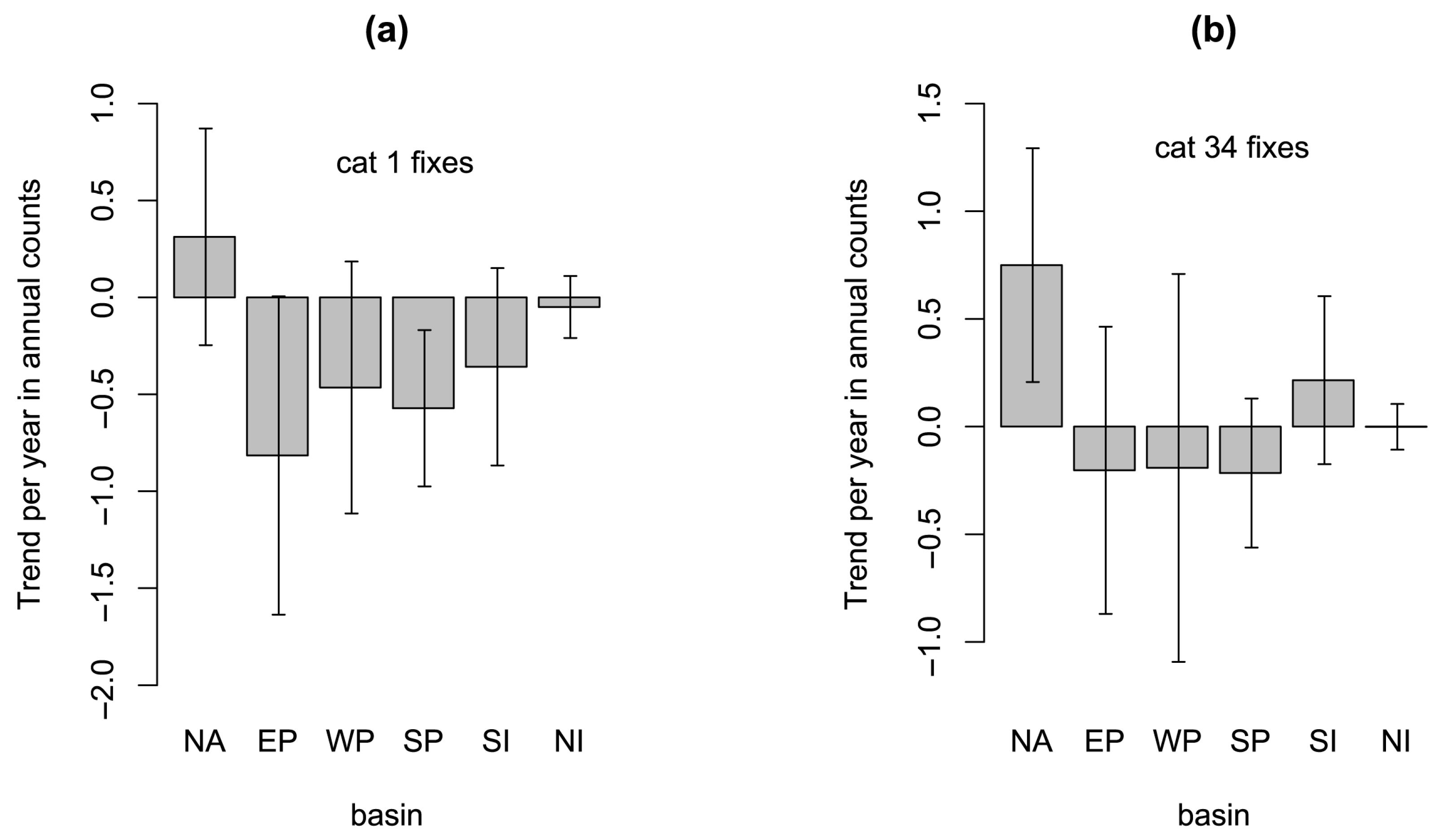
Figure 4a shows the trends in the number of cat1 fixes for these six regions. Corresponding time series are shown in Figure A1. We see that there is a positive trend in the North Atlantic, and negative trends everywhere else. The only significant trends are the negative trends in the EP and SP basins. We conclude that the significant negative trend in global cat1 fixes, which is driving the negative trend in global cat12 fixes, and which appears to be the most important factor driving the positive trend in the MH ratio, comes from all basins except the North Atlantic.
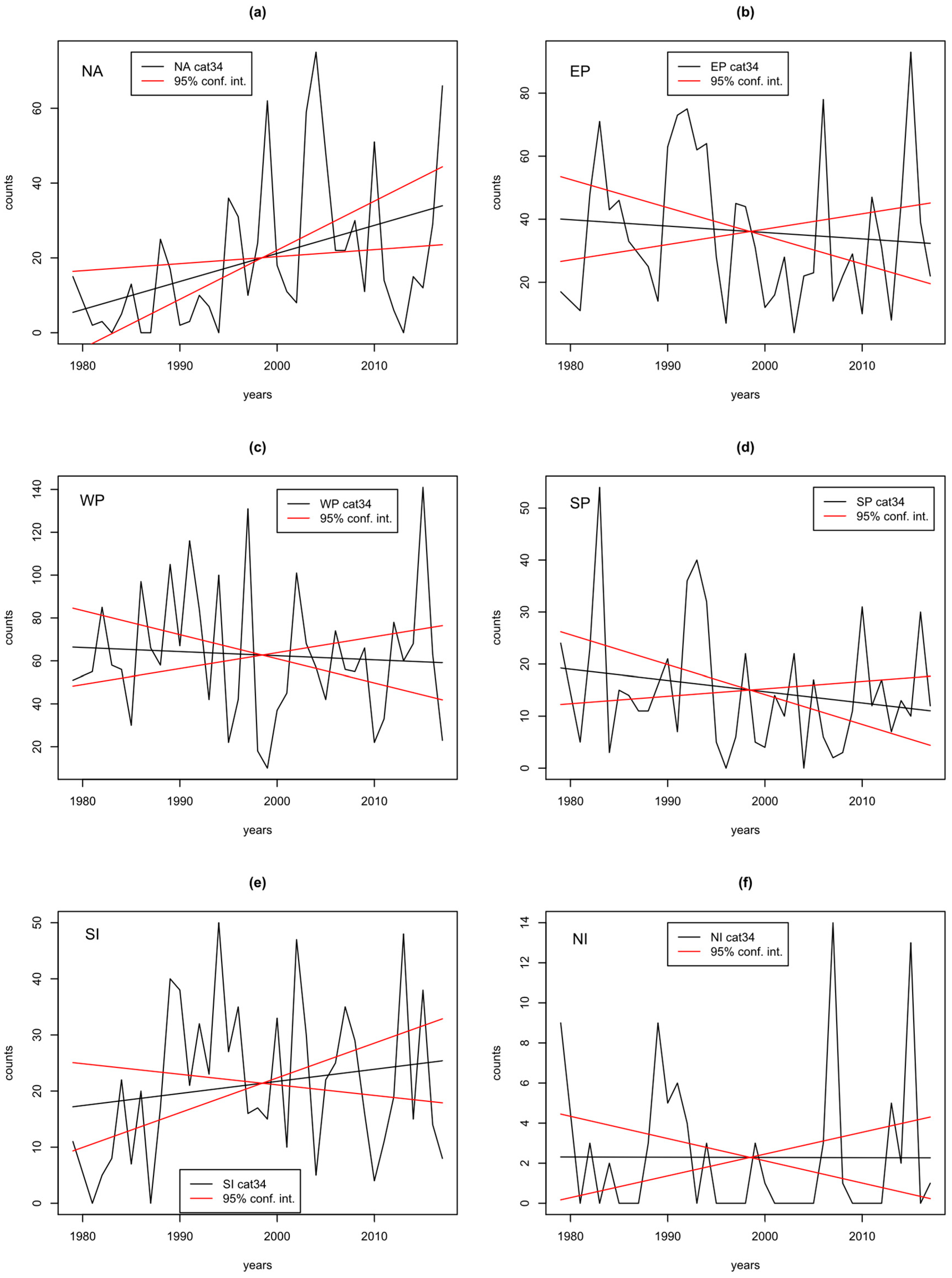
Figure 4b shows the trends in cat34 fixes by region. Corresponding time series are shown in Figure A2. We see that there is a significant positive trend in the North Atlantic, a non-significant smaller positive trend in the Southern Indian basin, essentially no trend in the Northern Indian basin, and non-significant negative trends in all other regions. We conclude that the positive trend in the global cat34 fixes, which is driving the positive trend in the global cat35 fixes, which is partly driving the positive trend in the MH ratio, comes almost entirely from the North Atlantic.
Overall, we can conclude, subject again to quantitative confirmation in Section 4 below, that the upward trend in the MH ratio seems to be driven mostly by a negative trend in cat1 fixes outside the North Atlantic, and to some extent by a positive trend in cat34 fixes in the Atlantic.
4. Quantitative Analysis
We now describe an analysis in which we decompose the trend in the MH ratio into various component terms, in order to make the heuristic analysis of the previous section quantitative.
4.1. Decomposition by Numerator and Denominator
In our first decomposition, we will decompose the trend in the MH ratio into a linear combination of trends in the numerator (cat35 fixes) and denominator (cat15 fixes), plus a residual. We will write as the trend slope of the MH ratio, as the trend slope of the number of cat35 fixes, as the trend slope of the number of cat15 fixes and as the trend slope of the number of cat12 fixes. In addition, we will write as the mean of the number of cat35 fixes, as the mean of the number of cat15 fixes, and . Then, using the standard OLS formulae for all the trend slopes, it is relatively simple to show that:
where is a residual term involving an infinite expansion of non-linear terms. This equation matches intuition in the sense that if the trend in the cat35 fixes increases then the trend in the MH ratio increases, while if the trend in the cat15 fixes increases then the trend in the MH ratio decreases. One way to understand this equation is that it approximates the trend in the MH ratio, expressed as a proportion (), in terms of the trend in cat35 fixes, expressed as a proportion (), minus the trend in the cat15 fixes, also expressed as a proportion (). Following the discussion about the impacts of observational errors in Section 2, the estimates of trends in the numbers of fixes in subsets of the data are likely more prone to the impacts of observational errors than the estimate of the trend in the MH ratio. In Equation (2), this may mean that there are errors in slopes and which cancel, to some extent, and hence contribute to less error in the slope . As a result, and also because of general variability in the number of tropical storm fixes, the percentages in this and all the subsequent decompositions should not be considered as highly precise estimates.
We calculated all four terms in the above expression (Equation (2)) and evaluated them as a percentage of the trend in the MH ratio . We find that the residual accounts for 1.0% of , indicating that the trend in the MH ratio is well approximated by a linear combination of the trends in the cat35 and cat15 fixes and . accounts for 23.0% of and accounts for 76.0% of .
This result confirms what we found in the heuristic analysis in the previous section: the upward trend in the MH ratio is driven mainly by the downward trend in the number of cat15 fixes, and partly by the upward trend in the number of cat35 fixes.
If instead we decompose the trend in the slope of the MH ratio into the trend in the slope of the cat35 fixes and the trend in the slope of the cat12 fixes , we find that
The residual remains the same, while now accounts for 14.9% of and accounts for 84.2% of . This result again confirms what we saw in the previous section: the upward trend in the MH ratio is driven mainly by the downward trend in the number of cat12 fixes, and only partly by the upward trend in the number of cat35 fixes. The downward trend in the cat12 fixes is between five and six times more important than the upward trend in cat35 fixes in determining the upward trend in the MH ratio. We should also bear in mind that the upward trend in the cat35 fixes is not significant and may not be robust.
4.2. Decomposition by Category of Storm
We can decompose the trend in the MH ratio further into contributions from the trends in every category of storm strength. We write , , , and as the OLS trends in the numbers of cat 1, 2, 3, 4 and 5 fixes. We can then decompose the MH ratio into components for each of these trend slopes and a non-linear residual as follows:
where . Applying this new decomposition, we find percent contributions from the 5 categories from 1 to 5 of 76%, 8%, 20%, 5%, and −10% (remembering that this finer level of decomposition is even more prone to errors due to variability and observational error). We see that by far the biggest contribution to the upward trend in the MH ratio comes from the downward trend in cat1 fixes (76%). The second biggest contribution by strength category comes from the upward trend in cat3 fixes (20%). This confirms what we were able to deduce heuristically from Figure 3 in the previous section.
4.3. Decomposition by Region
We can extend the above decomposition analysis even further and decompose the trend in the MH ratio into contributions for each of the five strength categories and six basins, giving 30 categories in all. The results are shown in Table 2 as percentage contributions to the trend in the MH ratio. Sizes of trends for each of the 30 categories are shown in Table 3. The numeric values in the first two columns of Table 2 and Table 3 are similar, but this is purely numeric coincidence. The percentage values in Table 2 add up to 102% because of rounding error. Combining the information from Table 2 and Table 3, we see that the biggest contributors to the upward trend in the MH ratio are downward trends in cat1 fixes in the three Pacific basins and the Southern Indian Ocean, and upward trends in cat34 fixes in the North Atlantic. Cat35 fixes in the Pacific basins show downward trends, which contribute negatively to the trend in the MH ratio (i.e., tend to counteract the positive upward trend in the ratio), and cat1 fixes in the North Atlantic show a positive trend that also contributes negatively to the trend in the ratio.
These results confirm what we previously deduced from Figure 4 in the previous section, which is that the upward trend in the MH ratio seems to be driven mostly by a negative trend in the cat1 fixes outside the North Atlantic (which is highly significant, with a p-value of 0.0035), and to some extent by a positive trend in cat34 fixes in the Atlantic (which is also significant, with a p-value of 0.01).
4.4. Regional Analysis of Ratios
Motivated by the results in Table 2 and Table 3, Table 4 shows trends for various different versions of the cat35/cat15 ratio, and their significance. The first column shows the ratio for all basins together, as has been discussed in Section 2 above. This trend is significant, as we have seen above. The second column shows the trend in the cat35/cat15 ratio for all regions excluding the North Atlantic. The North Atlantic shows upward trends in both cat12s and cat35s, but the upward trend in the cat35s is larger (driven by a strong upward trend in cat34s), and hence removing the North Atlantic reduces the trend in the ratio, and the trend, although still positive, is no longer significant. We see that the strong upward trend in the North Atlantic cat34s is an essential component in the significance of the trend in the global MH ratio. The third column shows the North Atlantic on its own, which shows a large and significant upward trend in the ratio. Of the other five basins, four show positive trends in the ratio, of which one is significant (the Southern Indian ocean), although these regional trends, even more than the global trends, must be understood in the context of the large uncertainties in the data [4]. From Table 3, we see that the upward trends in the ratio in the three Pacific basins are driven by large decreases in the number of cat1s which are not offset by simultaneous increases in cat35s. The changes in these basins would seem to be best described as reductions in overall tropical cyclone frequency, with small changes in the distribution of intensities. With regard to the robustness of the trend in the global MH ratio, we can say that the trend is robust to a certain extent: after removing the North Atlantic, the sign of the trend remains the same, even though the significance is lost, and those of the other basins mostly show the same sign of trend. Given the level of variability of tropical cyclone numbers, and the size of the trend that would be expected from modelling studies [3], one would not expect the trend to be completely robust to all these tests.
4.5. Discussion
Combining the results from Section 3 above and from this section, we draw the following conclusions:
- (1)
- The upward trend in the global MH ratio is mainly driven by a downward trend in the number of cat1 fixes in basins other than the North Atlantic.
- (2)
- A secondary and less important driver is the upward trend in the number of cat34 fixes in the North Atlantic. Although this driver is less important than the decrease in the cat1 fixes, without it the trend in the MH ratio is no longer significant.
- (3)
- Of the other five basins, only one shows a significant upward trend in the basin-level ratio (while noting that the trends in individual basins are subject to a greater extent to observational errors)
- (4)
- The small upward trend in global total cat35 fixes shown in Figure 2a does not reflect a uniform global increase in cat35 fixes, but is driven by the large increase in the North Atlantic, an increase in the Southern Indian Ocean, and decreases in the three Pacific basins.
On a global aggregate level, we see a pattern consisting of a decrease in weak tropical cyclone fix numbers and an increase in strong tropical cyclone fix numbers. This is consistent with the idea of increasing intensity of individual tropical cyclones with climate change. However, this effect is mostly driven by combining together different behaviors in the North Atlantic and the other basins, and it is generally accepted that the large recent increase in North Atlantic hurricane numbers is likely strongly affected by regional climate variability as well as climate change. Possible explanations for the trends in the North Atlantic include variations in anthropogenic aerosols [13,14], natural climate variability on multidecadal time-scales [15], and the effects of volcanic eruptions [14,16]. As a result, it is difficult to determine accurately to what extent the increase in the MH ratio is due to climate change and to what extent the increase is due to regional climate variability.
5. Conclusions
In a study based on the ADT-HURSAT database of global tropical cyclone observations, Kossin et al. [8] identified a statistically significant increasing trend in the ratio of the number of cat35 fixes to the number of cat15 fixes (the MH ratio). We have explored the origins of this trend in terms of trends in the underlying numbers of fixes by storm category and by region in order to inform decisions about how tropical cyclone risk models might be adjusted to reflect the trend, for risk modelers interested in making such an adjustment.
We find that the main driver of the trend in the MH ratio is a downward trend in the cat15 fixes, which itself is driven by a statistically significant downward trend in the number of cat12 fixes, which itself is mostly driven by a statistically significant downward trend in the number of cat1 fixes. That in turn is driven by a statistically significant downwards trend in the number of cat1 fixes outside the North Atlantic basin. The North Atlantic cat1 fixes show an increasing trend, unlike any other basin.
The downward trend in cat1 fixes has an implication for regions affected by tropical cyclones, which is that the number of cat1 fixes occurring today in all regions except the North Atlantic seems to be lower than in previous decades. Risk estimates outside the North Atlantic based on the average number of cat1 fixes over previous decades might be too high.
A secondary driver for the upward trend in the MH ratio is a weak and non-significant upward trend in the cat 35 fixes. This is driven by a strong and significant upward trend in the number of cat34 fixes in the North Atlantic, which counteracts a downward trend in the number of cat35 fixes on average over the other basins. The trend in the number of cat34 fixes also has implications for risk estimation. Risk estimates for the North Atlantic based on averages of numbers of cat34 fixes over previous decades might be too low.
All these results must be understood in the context of the uncertainties in the underlying data. For instance, as discussed in Kossin et al. [8], there are gaps in the data. While these gaps do not have a big impact on estimates of the MH ratio and the results presented in Kossin et al., they are likely to have a bigger impact on the estimates of trends in the numbers of fixes that we have presented here.
Based on the above results, there are various ways that risk modelers could make adjustments if they wished to incorporate the trend in the MH ratio into their models. One way would be to adjust the global numbers of cat35 and cat12 fixes uniformly across all basins, although this would ignore the strong regional signals described above. Another way would be to adjust the numbers of cat34 fixes in the Atlantic basin, and the numbers of cat1 fixes in other basins, since these are the regional signals that are the main drivers for the increase. Given the uncertainties, all such adjustments to risk models should perhaps be treated as exploratory sensitivity tests, to test the impact of different hypotheses, rather than as fully credible views of hurricane risk.
Author Contributions
Conceptualization, S.J.; methodology, S.J.; software, S.J.; validation, S.J., N.L.; formal analysis, S.J.; writing—original draft preparation, S.J.; writing—review and editing, S.J., N.L.; visualization, S.J. All authors have read and agreed to the published version of the manuscript.
Funding
This research received no external funding. The work was funded by the authors.
Acknowledgments
We would like to acknowledge the help of Jim Kossin, and the very helpful suggestions from three anonymous reviewers which greatly improved the manuscript.
Conflicts of Interest
The authors declare no conflict of interest.
Appendix A
Figure A1.
(a–f) show the number of cat1 fixes (black time series), with a linear trend (black line), and lines showing 95% confidence intervals on the trend slope, for 6 basins.
Figure A1.
(a–f) show the number of cat1 fixes (black time series), with a linear trend (black line), and lines showing 95% confidence intervals on the trend slope, for 6 basins.

Figure A2.
(a–f) show the number of cat34 fixes (black time series), with a linear trend (black line), and lines showing 95% confidence intervals on the trend slope for 6 basins.
Figure A2.
(a–f) show the number of cat34 fixes (black time series), with a linear trend (black line), and lines showing 95% confidence intervals on the trend slope for 6 basins.

References
- Emanuel, K. The dependence of hurricane intensity of climate. Nature 1987, 326, 483–485. [Google Scholar] [CrossRef]
- Sobel, A.; Camargo, S.; Hall, T.; Lee, C.; Tippett, M.; Wing, A. Human influence on tropical cyclone intensity. Science 2016, 353, 242–246. [Google Scholar] [CrossRef] [PubMed] [Green Version]
- Knutson, T.; Camargo, S.; Chan, J.; Emanuel, K.; Ho, C.; Kossin, J.; Mohapatra, M.; Satoh, M.; Sugi, M.; Walsh, K.; et al. Tropical cyclones and climate change assessment: Part II: Projected response to anthropogenic warming. Bull. Am. Meteorol. Soc. 2020, 101, E303–E322. [Google Scholar] [CrossRef]
- Landsea, C.; Harper, B.; Hoarau, K.; Knaff, J. Can we detect trends in extreme tropical cyclones? Science 2006, 313, 452–454. [Google Scholar] [CrossRef] [PubMed] [Green Version]
- Goldenberg, S.; Landsea, C.; Mestas-Nunez, A.; Gray, B. The Recent Increase in Atlantic Hurricane Activity: Causes and Implications. Science 2001, 293, 474–479. [Google Scholar] [CrossRef] [PubMed] [Green Version]
- Elsner, J.; Kossin, J.; Jagger, T. The increasing intensity of the strongest tropical cyclones. Nature 2008, 455, 92–95. [Google Scholar] [CrossRef] [PubMed]
- Knutson, T.; Camargo, S.; Chan, J.; Emanuel, K.; Ho, C.; Kossin, J.; Mohapatra, M.; Satoh, M.; Sugi, M.; Walsh, K.; et al. Tropical cyclones and climate change assessment: Part 1: Detection and attribution. Bull. Am. Meteorol. Soc. 2019, 100, 1987–2007. [Google Scholar] [CrossRef] [Green Version]
- Kossin, J.; Knapp, K.; Olander, T.; Velden, C. Global Increase in major tropical cyclone exceedance probability over the past four decades. Proc. Natl. Acad. Sci. USA 2020, 117, 11975–11980. [Google Scholar] [CrossRef] [PubMed]
- Kossin, J.; Olander, T.; Knapp, K. Trend analysis with a new global record of tropical cyclone intensity. J. Clim. 2013, 26, 9960–9976. [Google Scholar] [CrossRef]
- Knapp, K.R.; Kossin, J.P. New global tropical cyclone data from ISCCP B1 geostationary satellite observations. J. Appl. Remote Sens. 2007, 1, 013505. [Google Scholar]
- Knapp, K.; Kruk, K.; Levinson, D.; Diamond, H.; Neumann, C. The international best track archive for climate stewardship (IBTrACS): Unifying tropical cyclone best track data. Bull. Am. Meteorol. Soc. 2010, 91, 363–376. [Google Scholar] [CrossRef]
- Holland, G.; Bruyere, C. Recent intense hurricane response to global climate change. Clim. Dyn. 2014, 42, 617–627. [Google Scholar] [CrossRef] [Green Version]
- Dunstone, N.J.; Smith, D.M.; Booth, B.B.; Hermanson, L.; Eade, R. Anthropogenic aerosol forcing of Atlantic tropical storms. Nat. Geosci. 2013, 6, 534–539. [Google Scholar] [CrossRef]
- Murikami, H.; Delworth, T.L.; Cooke, W.F.; Zhao, M.; Xiang, B.; Hsu, P.C. Detected climatic change in global distribution of tropical cyclones. Proc. Natl. Acad. Sci. USA 2020, 117, 10706–10714. [Google Scholar] [CrossRef] [PubMed]
- Yan, X.; Zhang, R.; Knutson, T. The role of Atlantic overturning circulation in the recent decline of Atlantic major hurricane frequency. Nat. Commun. 2017, 8, 1695. [Google Scholar] [CrossRef] [PubMed] [Green Version]
- Pausata, F.S.; Camargo, S.J. Tropical cyclone activity affected by volcanically induced ITCZ shifts. Proc. Natl. Acad. Sci. USA 2019, 116, 7732–7737. [Google Scholar] [CrossRef] [PubMed] [Green Version]
Figure 1.
(a) shows numbers of cat15 (red), cat12 (black) and cat35 (blue) fixes from the ADT-HURSAT dataset, and (b) shows the ratio of cat35 to cat15 fixes (major hurricane (MH) ratio, black time series), with a fitted linear trend (black line), with lines showing 95% confidence limits (red). The linear trend is fitted using ordinary least squares (OLS) regression. The trend change is 7 percentage points over 39 years, and is significant with a p-value of 0.01. In the calculations, 1980 is treated as a missing value, and in the graph it is filled in using linear interpolation between 1979 and 1981.

Figure 2.
(a) shows numbers of cat35 fixes (black time series) (as in Figure 1a), with a linear trend (black line), and 95% confidence intervals trend (red lines). (b) shows cat12 in the same format; (c) shows cat 15 in the same format, and (d) shows the ratio of cat35 to cat12 in the same format.
Figure 2.
(a) shows numbers of cat35 fixes (black time series) (as in Figure 1a), with a linear trend (black line), and 95% confidence intervals trend (red lines). (b) shows cat12 in the same format; (c) shows cat 15 in the same format, and (d) shows the ratio of cat35 to cat12 in the same format.

Figure 3.
(a) shows the number of cat1 fixes (black time series), with a linear trend (black line), and lines showing 95% confidences on the trend slope; (b–e) show cat2, cat3, cat4 and cat5 fixes in the same format; (f) shows time series of all five categories: cat1 (black), cat2 (red), cat3 (blue), cat4 (green), cat5 (purple).

Figure 4.
(a) shows the trends in the number of cat1 fixes by basin with 95% confidence intervals, and (b) shows the trends in the number of cat34 fixes by basin with 95% confidence intervals. The time series to which these trends relate are shown in Figure A1 and Figure A2.


Table 1.
Trend slopes and significance levels for global trends in numbers of tropical cyclone fixes. The first column (Trend) shows trend slope values expressed as numbers of fixes per year. The second column (Significance) shows the p-value for significance of the trend.
Table 1.
Trend slopes and significance levels for global trends in numbers of tropical cyclone fixes. The first column (Trend) shows trend slope values expressed as numbers of fixes per year. The second column (Significance) shows the p-value for significance of the trend.
| Trend | Significance | |
|---|---|---|
| cat1 | −1.95 | 0.004 |
| cat2 | −0.20 | 0.54 |
| cat3 | 0.28 | 0.45 |
| cat4 | 0.08 | 0.86 |
| cat5 | −0.14 | 0.18 |
| cat12 | −2.15 | 0.02 |
| cat15 | −1.94 | 0.23 |
| cat35 | 0.21 | 0.79 |
Table 2.
Percentage contributions to the trend in the MH ratio, by region and storm category.
| cat1 | cat2 | cat3 | cat4 | cat5 | Total | |
|---|---|---|---|---|---|---|
| NA | −12 | −12 | 31 | 23 | 3 | 33 |
| EP | 32 | 6 | −7 | −7 | −1 | 23 |
| WP | 18 | 5 | 2 | −16 | −12 | −3 |
| SP | 23 | 8 | −10 | −5 | −1 | 15 |
| SI | 14 | 3 | 5 | 10 | 1 | 33 |
| NI | 2 | −1 | 0 | 0 | 0 | 1 |
| total | 77 | 9 | 21 | 5 | −10 | 102 |
Table 3.
Trends in the number of fixes, by category and region, in units of counts per 39 years.
| cat1 | cat2 | cat3 | cat4 | cat5 | Total | |
|---|---|---|---|---|---|---|
| NA | 12 | 12 | 17 | 13 | 1 | 55 |
| EP | −32 | −6 | −4 | −4 | −1 | −47 |
| WP | −18 | −4 | 1 | −9 | −6 | −36 |
| SP | −22 | −8 | −6 | −3 | 0 | −39 |
| SI | −14 | −3 | 3 | 6 | 1 | −7 |
| NI | −2 | 1 | 0 | 0 | 0 | −1 |
| total | −76 | −8 | 11 | 3 | −5 | −75 |
Table 4.
Fitted trends for various cat35/cat15 fixes ratios. The first row (Trend) shows trend values expressed as change in the ratio over 39 years. The second row (Significance) shows the p-value for significance of the trend. The first column (ALL) is for all regions combined. The second column (-NA) is for all regions excluding the North Atlantic.
| ALL | -NA | NA | EP | WP | SP | SI | NI | |
|---|---|---|---|---|---|---|---|---|
| Trend | 0.07 | 0.05 | 0.31 | 0.04 | 0.00 | 0.12 | 0.23 | −0.04 |
| Significance | 0.0099 | 0.0910 | 0.0036 | 0.4782 | 0.9735 | 0.1576 | 0.0003 | 0.7083 |
Publisher’s Note: MDPI stays neutral with regard to jurisdictional claims in published maps and institutional affiliations. |
© 2020 by the authors. Licensee MDPI, Basel, Switzerland. This article is an open access article distributed under the terms and conditions of the Creative Commons Attribution (CC BY) license (http://creativecommons.org/licenses/by/4.0/).
Share and Cite
MDPI and ACS Style
Jewson, S.; Lewis, N. Statistical Decomposition of the Recent Increase in the Intensity of Tropical Storms. Oceans 2020, 1, 311-325. https://0-doi-org.brum.beds.ac.uk/10.3390/oceans1040021
AMA Style
Jewson S, Lewis N. Statistical Decomposition of the Recent Increase in the Intensity of Tropical Storms. Oceans. 2020; 1(4):311-325. https://0-doi-org.brum.beds.ac.uk/10.3390/oceans1040021
Chicago/Turabian StyleJewson, Stephen, and Nicholas Lewis. 2020. "Statistical Decomposition of the Recent Increase in the Intensity of Tropical Storms" Oceans 1, no. 4: 311-325. https://0-doi-org.brum.beds.ac.uk/10.3390/oceans1040021